Capacity Analysis of Bidirectional AF Relay Selection with Imperfect Channel State Information

Recently, bidirectional relay network attracts a lot of interest, because it has better spectral efficiency than conventional one-way relay network when adopting the network coding technique[1]. In addition, the relay selection (RS) technique has been intensively researched in the bidirectional relay network, due to its ability to achieve full diversity with a single relay[2, 3, 4, 5]. In [2, 3], the symbol error rate (SER) of bidirectional RS was derived in a closed-form, which verifies that RS can achieve full diversity. The ergodic capacity analysis of bidirectional RS was obtained in [4, 5]. Furthermore, imperfect channel state information (CSI), i.e., outdated CSI and imperfect channel estimation, has great impact on the performance of RS, which has been fully studied in one-way relay network, such as the SER analysis [6, 7], and the ergodic capacity analysis [8, 9]. However, to the best of the authors’ knowledge, all the previous researches about bidirectional RS all assume the CSI is perfect, and the impact of imperfect CSI, such as outdated CSI, on the performance of bidirectional RS has not been investigated.

In this paper, we analyze the ergodic capacity of RS in bidirectional amplify-and-forward (AF) relay with imperfect CSI. The system model and the imperfect CSI model are presented in Section II. In Section III, we discuss the optimal RS scheme in maximizing the ergodic capacity. However, it cannot be achieved practically, due to the imperfect CSI. Therefore, two suboptimal RS schemes are analyzed, in which the first scheme is based on the imperfect channel coefficients, and the second scheme is based on the predicted channel coefficients. The tight lower bound of the ergodic capacity for the suboptimal RS schemes is derived in Section IV. It is noted that the analytical expression is provided under the generalized network structure, i.e., the channel coefficients follow independent but not necessarily identical complex-Gaussian fading, and the correlation coefficients of outdated CSI are different for different channels. In Section V, Monte-Carlo simulations verify that the analytical expression matches tightly with the simulated results. The results reveal that the ergodic capacity of bidirectional RS degrades greatly once CSI is imperfect, whereas the RS scheme based on the predicted channel can compensate the performance loss, and it approaches infinitely to the performance achieved by the optimal RS scheme, when the prediction length is sufficiently large.

Notation: $\left(\cdot\right)^{*}$, $\left(\cdot\right)^{T}$, and $\left(\cdot\right)^{H}$ represent the conjugate, the transpose, and the conjugate transpose, respectively. $\mathbb{E}$ is used for the expectation and $\Pr$ represents the probability.

In this paper, we investigate a generalized bidirectional AF relay network with two sources $S_{j}$, $j=1,2$, exchanging information through $N$ relays $R_{i}$, $i=1,\ldots,N$, where each node is equipped with a single half-duplex antenna. The transmit powers of each source and each relay are denoted by $p_{s}$ and $p_{r}$, respectively. The direct link between sources does not exist due to the shadowing effect, and the channel coefficients between $S_{j}$ and $R_{i}$ are reciprocal, denoted by $h_{ji}$. All the channel coefficients are independent complex-Gaussian random variables (RV) with zero mean and variance of $\sigma_{h_{ji}}^{2}$, and these coefficients are constant over the duration of one frame.

The whole procedure of bidirectional AF RS is divided into two parts periodically: relay selection process and data transmission process. During the relay selection process, e.g., the $\tau$th frame, the central unit (CU), i.e., $S_{j}$, selects the best relay according to the predefined RS scheme, which will be discussed in the next section. During the data transmission process, e.g., the $\big(\tau+\tau^{\prime}\big)$th frame, only the selected relay is used for transmission, and other relays keep idle until the next relay selection process comes. Due to the time-variation of channel, the channel at the date transmission process $h_{ji}\left(\tau+\tau^{\prime}\right)$ is quite different from that at the relay selection process $h_{ji}\left(\tau\right)$, and their relationship is modeled as [6]

where $\varepsilon_{ji}$ is an independent identically distributed RV with $h_{ji}\left(\tau\right)$; $\rho_{f_{ji}}=J_{0}\left(2\pi f_{d_{ji}}T\tau^{\prime}\right)$, where $J_{0}\left(\cdot\right)$ stands for the zeroth order Bessel function[12], $f_{d_{ji}}$ is the Doppler spread, and $T\tau^{\prime}$ is the time delay.

The imperfect channel estimation is also considered in this paper, and the channel $h_{ji}$ and its estimate $\hat{h}_{ji}$ are related by $h_{ji}=\hat{h}_{ji}+e_{ji}$[7], in which $\hat{h}_{ji}$ and the detection error $e_{ji}$ follow independent zero-mean complex-Gaussian distributions with variances of $\sigma_{\hat{h}_{ji}}^{2}$ and $\sigma_{e_{ji}}^{2}$, respectively, and $\sigma_{e_{ji}}^{2}=0$ means no estimation error.

Considering the transmission via $R_{i}$, the data transmission process of bidirectional AF relay is divided into two phases. During the first phase, the sources simultaneously send their respective information to $R_{i}$. The received signal at $R_{i}$ is $r_{i}=\sqrt{p_{s}}h_{t,1i}s_{1}+\sqrt{p_{s}}h_{t,2i}s_{2}+n_{ri}$, where $h_{t,ji}\mathrel{\mathop{\kern 0.0pt=}\limits^{\Delta}}h_{ji}\left(\tau+\tau^{\prime}\right)$, $s_{j}$ denotes the modulated symbols transmitted by $S_{j}$ with the average power normalized, and $n_{ri}$ is the additive white Gaussian noise (AWGN) at $R_{i}$, which is zero mean and variance of $\sigma_{n}^{2}$. During the second phase, $R_{i}$ amplifies and forwards the received signal back to the sources. The signal generated by $R_{i}$ satisfies $t_{i}=\sqrt{p_{r}}\beta_{i}r_{i}$, where $\beta_{i}=\left(p_{s}\hat{\gamma}_{t,1i}+p_{s}\hat{\gamma}_{t,2i}+\sigma_{n}^{2}\right)^{-1/2}$ is the variable-gain factor[6], and $\hat{\gamma}_{t,ji}=|\hat{h}_{t,ji}|^{2}$. The received signal at $S_{j}$ via $R_{i}$ is $y_{ji}=h_{t,ji}t_{i}+n_{sj}$, where $n_{sj}$ is the AWGN at $S_{j}$. After reconstructing and canceling the self-interference, i.e., $\sqrt{p_{s}p_{r}}\beta_{i}\hat{h}_{t,ji}\hat{h}_{t,ji}s_{j}$[3], the instantaneous received signal-plus-interference-to-noise ratio (SINR) at $S_{j}$ via $R_{i}$ is

where $\psi_{s}=p_{s}/\sigma_{n}^{2}$, $\psi_{r}=p_{r}/\sigma_{n}^{2}$, $\tilde{\psi}_{s}=\psi_{s}+\psi_{s}\psi_{r}\sigma_{e_{ji}}^{2}$, $\tilde{\psi}_{r}=\psi_{r}+3\psi_{s}\psi_{r}\sigma_{e_{ji}}^{2}+\psi_{s}\psi_{r}\sigma_{e_{{\bar{j}}i}}^{2}$, $c=2\psi_{r}\psi_{s}\sigma_{e_{ji}}^{4}+\psi_{r}\psi_{s}\sigma_{e_{\bar{j}i}}^{4}+\psi_{r}\sigma_{e_{ji}}^{2}+1$, and $\{j,\overline{j}\}=\{1,2\}~\mbox{or}~\{2,1\}$.

The ergodic capacity of the bidirectional RS is defined as[4, 5]

where $k$ in the index of the selected relay, $\gamma_{jk}$ can be obtained by (2), and the pre-log factor $1/2$ means that the transmission of one data block from one source to the other occupies two phases.

To maximize the ergodic capacity, the optimal RS scheme is

where the detailed explanation of the scheme is given in Appendix A.

However, $\hat{h}_{ji}\left(\tau+\tau^{\prime}\right)$ is unknown at the relay selection process, due to the time-variation of channel (1). Accordingly, the optimal RS scheme (4) cannot be achieved with outdated CSI, thus we discuss two suboptimal RS schemes which can be implemented practically.

The first alternative RS scheme with outdated CSI is obtained by substituting the channel $\hat{h}_{ji}\left(\tau+\tau^{\prime}\right)$ in (4) with the outdated channel $\hat{h}_{ji}\left(\tau\right)$ obtained at the relay selection process[2, 4], i.e.,

The second alternative RS scheme with outdated CSI is obtained by substituting the channel $\hat{h}_{ji}\left(\tau+\tau^{\prime}\right)$ in (4) with its predicted value $h_{p,ji}\left(\tau+\tau^{\prime}\right)$, i.e.,

In this paper, the Wiener filter [13] is applied for channel prediction, which is the linear optimal prediction in minimizing the mean square error, thus we have $h_{p,ji}\big({\tau+\tau^{\prime}}\big)={\bf{w}}_{opt,ji}^{H}{\bf{\tilde{h}}}_{ji}$, where ${\bf{\tilde{h}}}_{ji}=\big[\hat{h}_{ji}\big(\tau\big),\hat{h}_{ji}\big(\tau-\Delta\big),\cdots,\hat{h}_{ji}\big(\tau-L_{ji}\Delta+\Delta\big)\big]^{T}$ contains the current and previous $\left(L_{ji}-1\right)$ channel coefficients, which are obtained from previous relay selection processes, $\Delta$ is the interval of adjacent relay selection processes in frames, $L_{ji}$ is the prediction length, and ${\bf{w}}_{opt,ji}={{\bf{R}}_{ji}^{-1}}{\bf{r}}_{ji}$, in which ${\bf{R}}_{ji}=\mathbb{E}\left\{{\bf{\tilde{h}}}_{ji}{\bf{\tilde{h}}}_{ji}^{H}\right\}$ and ${\bf{r}}_{ji}=\mathbb{E}\left\{{\bf{\tilde{h}}}_{ji}{h_{t,ji}^{*}}\right\}$. According to [13], $h_{ji}\left(\tau+\tau^{\prime}\right)=h_{p,ji}\left(\tau+\tau^{\prime}\right)+\sqrt{\sigma_{h_{ji}}^{2}-\sigma_{p_{ji}}^{2}}n_{ji}$, where $h_{p,ji}\left(\tau+\tau^{\prime}\right)$ is a complex-Gaussian RV with zero mean and variance of $\sigma_{p_{ji}}^{2}={\bf{r}}_{ji}^{H}{\bf{R}}_{ji}^{-1}{\bf{r}}_{ji}$, $n_{ji}$ is an independent complex-Gaussian RV with zero mean and unit variance. The normalized correlation coefficient between $h_{p,ji}\left(\tau+\tau^{\prime}\right)$ and $h_{ji}\left(\tau+\tau^{\prime}\right)$ satisfies $\rho_{p_{ji}}=\sqrt{\sigma_{p_{ji}}^{2}/\sigma_{h_{ji}}^{2}}$.

For simplicity, the notation $\hat{h}_{s,ji}$ is used to represent $\hat{h}_{ji}\left(\tau\right)$ and $h_{p,ji}\left(\tau+\tau^{\prime}\right)$. Specifically, for the RS scheme (5), $\hat{h}_{s,ji}\mathrel{\mathop{\kern 0.0pt=}\limits^{\Delta}}\hat{h}_{ji}\left(\tau\right)$, and for the RS scheme (6), $\hat{h}_{s,ji}\mathrel{\mathop{\kern 0.0pt=}\limits^{\Delta}}h_{p,ji}\left(\tau+\tau^{\prime}\right)$, then $\hat{\gamma}_{s,ji}\mathrel{\mathop{\kern 0.0pt=}\limits^{\Delta}}|\hat{h}_{s,ji}|^{2}$. With the unified notation $\hat{h}_{s,ji}$, the analysis of the RS schemes (5) and (6) can be expressed in a unified manner.

To analyze the ergodic capacity of bidirectional AF RS in (3), the distribution functions of $\hat{\gamma}_{t,jk}=\left|{\hat{h}_{j{k}}}\left(\tau+\tau^{\prime}\right)\right|^{2}$ in (2) need to be obtained first.

Lemma 1: According to the RS schemes and the relationship between $\hat{h}_{t,ji}$ and $\hat{h}_{s,ji}$, the PDF of $\hat{\gamma}_{t,j{k}}$ is expressed as

where

In addition, $\sum_{A_{t}}$ is the abbreviation of $\sum_{\scriptstyle A_{t}\subseteq\left\{{1,\ldots,N}\right\}\backslash i\hfill\atop\scriptstyle\left|{A_{t}}\right|=t\hfill}$, and $\left|{A_{t}}\right|$ represents the cardinality of set $A_{t}$. Moreover, $\sigma_{s,ji}^{2}$ and $\sigma_{t,ji}^{2}$ are the variances of $\hat{h}_{s,ji}$ and $\hat{h}_{t,ji}$, respectively. Specifically, for the RS scheme (5), $\sigma_{s,ji}^{2}=\sigma_{\hat{h}_{ji}}^{2}$, $\sigma_{t,ji}^{2}=\sigma_{\hat{h}_{ji}}^{2}$, $\rho_{ji}=\rho_{e}\rho_{f_{ji}}$, and $\rho_{e}=\sigma_{\hat{h}_{ji}}^{2}/\sigma_{h_{ji}}^{2}$[7]; for the RS scheme (6), $\sigma_{s,ji}^{2}=\sigma_{p_{ji}}^{2}$, $\sigma_{t,ji}^{2}=\sigma_{\hat{h}_{ji}}^{2}$, and $\rho_{ji}=\rho_{e}\rho_{p_{ji}}$. Also, $\sigma_{s,i}^{2}=\sigma_{s,1i}^{2}\sigma_{s,2i}^{2}/\big(\sigma_{s,1i}^{2}+\sigma_{s,2i}^{2}\big)$.

Proof: The derivation is given in Appendix B. $\hfill\blacksquare$

Lemma 2:

where $\varphi\left({a,b}\right)\mathrel{\mathop{\kern 0.0pt=}\limits^{\Delta}}\int\limits_{0}^{\infty}{\ln\left({x+a}\right)e^{-bx}dx}=\frac{{\ln a+e^{ab}E_{1}\left({ab}\right)}}{b}$[14, 4.337], and $E_{1}\left(x\right)$ is the exponential integral function [12].

Proof: Lemma 2 can be achieved by applying the integration by part, then discussing under the situations that $m=n$ and $m\neq n$. $\hfill\blacksquare$

Proposition 1 : Applying the Lemma 1 and Lemma 2, the ergodic capacity of bidirectional AF RS is

where

In addition, $m=\tilde{\psi}_{s}/\psi_{s}$, and $n=\big(\tilde{\psi}_{s}+\tilde{\psi}_{r}\big)/\psi_{r}$. $\xi^{\prime}_{j}$ and $\zeta^{\prime}_{j}$ can be obtained by $\xi_{j}$ and $\zeta_{j}$, respectively, by substituting $i,l,A_{t}$ in (8) and (9) with $i^{\prime},l^{\prime},A_{t^{\prime}}$, respectively, and $\{j,\overline{j}\}=\{1,2\}~\mbox{or}~\{2,1\}$.

It is noted that for the symmetric network structure, i.e., $\sigma_{h_{ji}}^{2}=1$, $\rho_{ji}=\rho$, $i=1,\ldots,N$, $j=1,2$, we have $\sum_{A_{t}}=\binom{N-1}{t}$, and $\sum_{A_{t}^{\prime}}=\binom{N-1}{t^{\prime}}$, thus the expression of capacity in Proposition 1 can be further simplified.

Proof: The derivation is given in Appendix C. $\hfill\blacksquare$

In this section, Monte-Carlo simulations are provided to validate the preceding analysis and to highlight the performance of bidirectional AF RS with outdated CSI. Without loss of generality, the sources and the relays are assumed to have the same transmit powers, i.e., $p_{s}=p_{r}=P_{0}$. The network structure is assumed to be symmetric, i.e., $\sigma_{h_{ji}}^{2}=1$ and $f_{d_{ji}}=f_{d}$, $j=1,2$, $i=1,\ldots,N$.

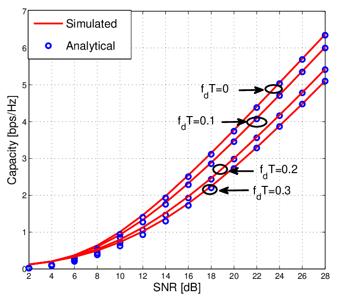
Fig. 1 studies the impact of outdated CSI on the ergodic capacity when $N=4$ and adopting the RS scheme (5). The x-axis is $\mbox{SNR}=P_{0}/\sigma_{n}^{2}$, and the imperfect estimation is considered, i.e., the variance of detection error $\sigma_{e}^{2}=\sigma_{n}^{2}/P_{0}$[10]. Different lines are provided under different $f_{d}T$, where larger $f_{d}T$ means CSI is outdated more severely than smaller $f_{d}T$, and $f_{d}T=0$ means CSI is not outdated. The figure verifies that the expression of Proposition 1 is the tight lower bound of the simulated results. We also observe that the ergodic capacity degrades once CSI is outdated, e.g., the performance loss between $f_{d}T=0.3$ and $f_{d}T=0$ is about $4$ dB in high SNR, and more severely outdated CSI results in greater performance loss, although outdated CSI has no impact on the multiplexing gain.

Figs. 2-4 study the capacity of bidirectional AF RS with outdated CSI, when adopting the RS scheme (6) and the variance of detection error $\sigma_{e}^{2}=0$. We assume the time interval between relay selection process and its subsequent data transmission process satisfies $\tau^{\prime}=1$, and the time interval between adjacent relay selection processes satisfies $\Delta=2$. The prediction lengths of different channels are assumed to be the same, i.e., $L_{ji}=L$, $j=1,2$, $i=1,\ldots,N$.

Fig. 2 plots the simulated and the analytical ergodic capacity of outdated CSI versus $\mbox{SNR}=P_{0}/\sigma_{n}^{2}$, when the coefficient of outdated CSI is fixed, i.e., $f_{d}T=0.3$. The simulated results verify the lower bound in Proposition 1 is tight when the channel prediction is adopted. For the symmetric network, the line of $L=1$ represents the RS scheme (5), because $\rho_{p}=\rho_{f}$ when $L=1$. Also, the line of $L=\infty$ means the CSI is perfect, because $\rho_{p}=1$ when $L=\infty$. As this figure reveals, the RS scheme based on channel prediction (6) outperforms the scheme without channel prediction (5), and the performance gain gets larger when increasing the prediction length. The qualitative explanation of the phenomenon is that increasing the prediction length results in growing the correlation coefficient $\rho_{p}$, thus the prediction becomes more accurate and the performance gets improved.

Fig. 3 investigates the impact of $f_{d}T$ on capacity when $\mbox{SNR}=10$, $15$, and $20$ dB. As the figure reveals, the curves of capacity under different prediction lengths $L$ have almost the same performance in small $f_{d}T$, and all the capacity degrades as $f_{d}T$ increases. However, larger $L$ has better robustness of capacity, e.g., for $L=1$ and SNR = $15$ dB, capacity degrades to $3$ bps/Hz when $f_{d}T=0.18$, whereas for $L=2$, it is $f_{d}T=0.27$ when capacity degrades to the same level. Therefore, larger $L$ improves the robustness of capacity.

Fig. 4 investigates the impact of prediction length $L$ on the capacity. The y-axis is the normalized difference of capacity, i.e., the difference between the capacity obtained by the RS scheme (6) and the capacity obtained by the optimal RS scheme (4), normalized by the latter. Smaller normalized difference means the capacity of the RS scheme (6) with outdated CSI has closer performance with the optimal performance. Different lines of Fig. 4 are plotted under different $f_{d}T$ and SNR, and all the normalized differences decrease monotonously to zero as $L$ increases, which reveals that the RS scheme (6) can infinitely approach to the optimal performance, by enlarging the prediction length. Furthermore, the results also reveal that the lines with larger $f_{d}T$ needs larger $L$ to satisfy the same need of the normalized difference.

The impact of imperfect CSI on the ergodic capacity of bidirectional AF RS has been investigated in this paper. The tight lower bound of ergodic capacity is derived in a closed form and verified by simulations. The results reveal that imperfect CSI will jeopardize the capacity of bidirectional RS network, whereas the RS based on the channel prediction can compensate the performance loss, and it can infinitely approach to the optimal performance, by enlarging the prediction length.

To maximize the ergodic capacity of (3) is equivalent to maximize $\gamma_{1i}\gamma_{2i}$, according to the approximation $\log_{2}\big(1+\gamma_{ji}\big)\approx\log_{2}\gamma_{ji}$, in which $\gamma_{ji}$ is provided in (2). Using the approximation $xy/\big(x+y+c\big)\approx\min\big(x,y\big)$, $\gamma_{1i}\gamma_{2i}$ is bounded by $\min\big(|\hat{h}_{t,1i}|^{2},|\hat{h}_{t,2i}|^{2}\big)^{2}$. Therefore, (3) is optimal in maximizing the capacity.

Similar to [6], the PDF of $\hat{\gamma}_{t,1k}$ can be expressed as

where (a) is satisfied by the total probability theorem, which divides the union event $\hat{\gamma}_{t,1k}<z$ into $N$ disjoint events, i.e., $R_{i}$ is the best relay and $\hat{\gamma}_{t,1i}<z$, $i=1,\ldots,N$; (b) is fulfilled by the division of two disjoint events, i.e., $\hat{\gamma}_{s,1i}>\hat{\gamma}_{s,2i}$ and $\hat{\gamma}_{s,1i}\leq\hat{\gamma}_{s,2i}$. Furthermore, $I_{1}$ and $I_{2}$ can be obtained by the definition of the RS schemes (5) and (6), the order statistics, and [11, eq. 26]. Substituting the exponential distributions of $\hat{\gamma}_{s,1i}$ and $\hat{\gamma}_{s,2i}$ into (15), Lemma 1 is verified by applying the conditional PDF of $\hat{\gamma}_{t,1k}$ and $\hat{\gamma}_{s,1k}$ and [14, eq. 6.614.3]. Moreover, the PDF of $\hat{\gamma}_{t,2k}$ can be obtained similarly.

The ergodic capacity of bidirectional RS is tightly bounded by

where $m=\tilde{\psi}_{s}/\psi_{s}$, and $n=\big(\tilde{\psi}_{s}+\tilde{\psi}_{r}\big)/\psi_{r}$. Comparing with (2), $(a)$ is achieved by adding the constant $mn-c$ in the dominator of (16), which has little effect on the performance, like the SER analysis [3].

After some manipulation of the logarithmic and expectation operations, the capacity of (16) is rewritten as $\overline{C}=\frac{T_{1}+T_{2}-T_{3}-T_{4}}{2\ln 2}$, where $T_{1}={\mathbb{E}_{\hat{\gamma}_{t,1k}}\big\{{\ln\left({\psi_{r}\hat{\gamma}_{t,1k}+m}\right)\hskip-2.27621pt+\hskip-2.27621pt\ln\left({\psi_{s}\hat{\gamma}_{t,1k}\hskip-2.27621pt+n}\right)}\big\}}$, and $T_{2}$ can be obtained by substituting $\hat{\gamma}_{t,1k}$ in $T_{1}$ with $\hat{\gamma}_{t,2k}$. According to the fact that $f_{Y}\left(z\right)=f_{X}\left(z/m\right)/m$ when $Y=mX\left(m>0\right)$, the PDFs of $\psi_{s}\hat{\gamma}_{t,jk}$ and $\psi_{r}\hat{\gamma}_{t,jk}$ can be obtained by the PDF of $\hat{\gamma}_{t,jk}$, $j=1,2$, then (13) can be achieved by Lemmas 1 and 2. Moreover, $T_{3}={\mathbb{E}_{\hat{\gamma}_{t,1k},\hat{\gamma}_{t,2k}}\bigg\{{\ln\Big[{\left(\tilde{\psi}_{s}\hskip-2.27621pt+\hskip-2.27621pt\tilde{\psi}_{r}\right)\hat{\gamma}_{t,1k}\hskip-2.27621pt+\hskip-2.27621pt\tilde{\psi}_{s}\hat{\gamma}_{t,2k}\hskip-2.27621pt+mn}\Big]}\bigg\}}$, and $T_{4}$ can be obtained by permuting $\hat{\gamma}_{t,1k}$ with $\hat{\gamma}_{t,2k}$ in $T_{3}$. $\hat{\gamma}_{t,1k}$ and $\hat{\gamma}_{t,2k}$ are independent RVs, thus the PDF of $\left(\tilde{\psi}_{s}+\tilde{\psi}_{r}\right)\hat{\gamma}_{t,1k}+\tilde{\psi}_{s}\hat{\gamma}_{t,2k}$ can be achieved by the convolution of $\left(\tilde{\psi}_{s}+\tilde{\psi}_{r}\right)\hat{\gamma}_{t,1k}$’s and $\tilde{\psi}_{s}\hat{\gamma}_{t,2k}$’s PDFs, then $T_{3}$ in (14) can also be achieved by Lemmas 1 and 2. The expression of $T_{4}$ can be obtained similarly.

References

• [1] P. Popovski and H. Yomo, “Wireless network coding by amplify-andforward for bi-directional traffic flows,” IEEE Commun. Lett., vol. 11, no. 1, pp. 16–18, Jan. 2007.
• [2] Y. Jing, “A relay selection scheme for two-way amplify-and-forward relay networks,” in Proc. Int. Conf. Wireless Commun. &\& Signal Process., Nov. 2009.
• [3] L. Song, “Relay selection for two-way relaying with amplify-and-forward protocols,” IEEE Trans. Veh. Technol., vol. 60, no. 4, pp. 1954–1959, May 2011.
• [4] P. K. Upadhyay and S. Prakriya, “Performance of two-way opportunistic relaying with analog network coding over Nakagami-m fading,” IEEE Trans. Veh. Technol., vol. 60, no. 4, pp. 1965–1971, May 2011.
• [5] K. Hwang, Y. Ko, and M.-S. Alouini, “Performance bounds for two-way amplify-and-forward relaying based on relay path selection,” in Proc. Veh. Technol. Conf., Apr. 2009.
• [6] D. S. Michalopoulos, H. A. Suraweera, G. K. Karagiannidis, and R. Schober, “Amplify-and-forward relay selection with outdated channel estimates,” IEEE Trans. Commun., vol. 60, no. 5, pp. 1278–1290, May 2012.
• [7] M. Seyfi, S. Muhaidat, J. Liang, and M. Dianati, “Effect of feedback delay on the performance of cooperative networks with relay selection,” IEEE Trans. Wireless Commun., vol. 10, no. 12, pp. 4161–4171, Dec. 2011.
• [8] M. Torabi and D. Haccoun, “Capacity analysis of opportunistic relaying in cooperative systems with outdated channel information,” IEEE Commun. Lett., vol. 14, no. 12, pp. 1137–1139, Dec. 2010.
• [9] H. Chen, J. Liu, Z. Dong, Y. Zhou, and W. Guo, “Exact capacity analysis of partial relay selection under outdated csi over Rayleigh fading channels,” IEEE Trans. Veh. Technol., vol. 60, no. 8, pp. 4014–4018, Oct. 2011.
• [10] S. S. Ikki and S. Aissa, “Two-way amplify-and-forward relaying with Gaussian imperfect channel estimations,” IEEE Commun. Lett., vol. 16, no. 7, pp. 956–959, Jul. 2012.
• [11] D. Ding, J. Ge, D. B. Costa, and Z. Jiang , “A new efficient low-complexity scheme for multi-source multi-relay cooperative networks,” IEEE Trans. Veh. Technol., vol. 60, no. 2, pp. 716–722, Feb. 2011.
• [12] M. Abramowitz and I. A. Stegun, Handbook of mathematical functions with formulas, graphs, and mathematical tables, 9th Edition, NewYork: Dover, 1970.
• [13] S. Haykin, Adaptive Filter Theory, 4th Edition, Prentice Hall Inc., 2002.
• [14] I. S. Gradshteyn and I. M. Ryzhik, Table of integals, series, and products, 5th Edition, Academic Press, 1994.
Refer to caption
Fig. 1: Capacity under outdated CSI when applying the scheme (5).
Fig. 2: Capacity when applying the RS scheme (6).
Fig. 3: The impact of fd​Tf_{d}T on the capacity.
Fig. 4: The normalized difference of capacity versus prediction length LL.