Extending the Hyades
Abstract
We explore the implications of models of the Hyades moving group in which it has a resonant origin, for regions of the Galaxy beyond the Solar neighbourhood. We show that while models associated with different resonances can produce nearly identical substructure in the local velocity distribution, the velocity distribution away from the Solar neighbourhood has different properties for different models. In particular there is a variation between different models of where in Galactocentric radius the observed Hyades signal in velocity space is strongest, at a given Galactic azimuth. We note, however, that the uncertainties in currently available data, primarily due to uncertain distances to stars, hide these signatures rather effectively, meaning we are not yet able to determine which resonance is the cause of the Hyades.
Keywords:
solar neighbourhood – Galaxy: kinematics and dynamics1 Introduction
It is well established that the velocity distribution in the Solar neighbourhood is far from smooth. The existence of “moving groups” of stars with similar velocities in the Solar neighbourhood has been recognised for over a hundred years (Kapteyn, 1905; Eggen, 1996, and references therein), but it was generally believed that these groups are composed of stars from dissolved clusters, which retain similar velocities (at a given point in the Galaxy) while spreading in space.
Using observations by the Hipparcos satellite (ESA, 1997), Dehnen (1998) showed that these moving groups dominate the distribution of blue () stars, and contain a substantial proportion of the redder stars in the Solar Neighbourhood (beyond Parengo’s discontinuity, ), with the same moving groups being seen in the velocity distributions of the different subsamples of Solar Neighbourhood stars. This suggested that a single moving group contains stars of many different ages, a result confirmed by Famaey et al. (2005), who added to the Hipparcos data by determining radial velocities for a sample of Hipparcos stars, allowing them to directly associate a given star with a given moving group. Comparison of these stars to isochrones in the Hertzsprung-Russell diagram then revealed the wide range of ages in each moving group. This is a very strong argument that moving groups must have dynamical origins. More recently, Pompéia et al. (2011) used chemical “tagging” to show that a large fraction of the stars in the Hyades moving group can not have originated from the Hyades cluster.
The dynamical processes that shape the velocity distribution of the Solar neighbourhood in to moving groups is still unclear. Kalnajs (1991) suggested that the Hyades and Sirius moving groups could be associated with an outer Lindblad resonance with the Galactic bar,11 1 In the discussion section of these conference proceedings, Kalnajs (questioned by Lindblad) concedes that the same structure in the velocity space at a single point could be produced by an inner Lindblad resonance with some unknown perturbation, but notes “I could tell the difference if I knew the stellar velocity distribution in a large enough region around the sun. But I will never know that.” while Dehnen (1999; 2000) used test-particle simulations to show how this resonance with the bar could instead produce the Hercules moving group (which is at velocities further from the circular velocity than the Hyades or Sirius groups, and was not fully recognised when Kalnajs was writing). Fux (2001) came to a similar conclusion, and more recently Minchev et al. (2010) argued that the moving groups at velocities near to the circular velocity may also be due to the influence of the bar’s OLR. Other work, beginning with De Simone, Wu, & Tremaine (2004), has looked at the possible influence of spiral structure, and shown that it is capable of producing a variety of substructures in velocity space, including those observed in the Solar Neighbourhood (Quillen & Minchev, 2005; Antoja et al., 2011; Pompéia et al., 2011, e.g). Other studies have sought to explain at least some of the moving groups as the response of the disc to the accretion of a satellite galaxy (Quillen et al., 2009; Minchev et al., 2009) or as the debris of an accreted satellite (Helmi et al., 2006, though this is only plausible for the higher velocity moving groups). All of these works used some form of test particle integration or N-body simulation to model the effects of these perturbations and their resonances.
More recent work has used angle-action coordinates to show that the Hyades moving group22 2 Throughout this paper we will refer to dynamical structure associated with the Hyades moving group as “the Hyades” in the interests of brevity. This should not be interpreted as meaning the Hyades star cluster, which is part of the moving group, but certainly doesn’t extend beyond the Solar neighbourhood! is associated with trapping at a Lindblad resonance (Sellwood, 2010). However, it is not clear which resonance is responsible, as very different resonances are associated with very similar structures in the velocity distribution of the Solar neighbourhood (McMillan, 2011b, henceforth M11). It is this approach that we pursue in this study, because it allows us to create easily tuneable models which make no assumptions about the nature of the perturber.
Recently it has become feasible to examine the velocity distribution of stars some distance away from the Solar neighbourhood. Notably (Antoja et al., 2012, henceforth A12) used observations by the RAdial Velocity Experiment (Steinmetz et al., 2006, RAVE: ) to investigate the velocity distribution in fields up to from the Sun, in the anti-rotation direction. In a spatial bin located around the Sun’s Galactocentric radius, but at least away in the Galactic azimuthal direction, they found a structure in velocity space at a similar position to that occupied by the Hyades in the Solar neighbourhood, as well as other overdensities at other points in velocity space. In other spatial bins which lie at similar Galactic azimuths, but at least inside or outside the Solar radius, they find no such structure at the velocity of the Hyades, but still find other substructure in velocity space.
In this paper we extend the models used by M11 to explore the implications of the expected velocity distributions away from the Solar neighbourhood. In Section 2 we discuss the nature of the resonances considered and the use of angle-action coordinates in describing them. In Section 3 we give the numerical details of the Hyades models that we test, before describing their properties away from the Solar neighbourhood in Section 4.
2 Angle-action coordinates and Lindblad resonances
Three actions and three conjugate angle coordinates provide exceptionally convenient coordinates for objects orbiting in a stationary or slowly evolving gravitational potential (and natural coordinates for perturbation theory). The actions are conserved quantities and the angles increase linearly with time, , where is a frequency. This means that can be thought of as labeling an orbit, and as describing a point on that orbit. The usual phase space coordinates are -periodic in each angle coordinate . For a phase-mixed distribution function (df) the distribution of stars is uniform in angle and therefore the df .
The conversion between the coordinate systems and is only known analytically for a few types of gravitational potential. However we can use the “torus fitting” method (e.g. McMillan & Binney, 2008, and references therein) to approximately find this conversion in an axisymmetric Galactic potential. This is done numerically, on an orbit-by-orbit basis – i.e. for a given the torus fitting algorithm finds an expression giving the values of for any , but a new torus fit has to be performed to know this relationship ( for any ) for a different .
In this study we work under the approximation that we can ignore the influence of the non-axisymmetric structure of the disc except for their trapping stars around resonances. This means that we can use the angles and actions calculated in the underlying axisymmetric potential, but that the df is reshaped by resonant trapping, and is not simply but also depends on the angles. This reshaping produces the Hyades.
Sellwood (2010) explored the distribution of the Solar neighbourhood stars in angle-action coordinates (under similar approximations), using data from the Geneva Copenhagen Survey (Holmberg, Nordström, & Andersen, 2009, GCS, ). The distribution of stars in action showed a clear indication that the Hyades moving group was associated with a resonance between the radial and azimuthal orbital frequencies of the stars ( and , both of which are functions of ) associated with a perturbation whose pattern speed satisfies
| (1) |
defines the type of resonance, with for an outer Lindblad resonance (OLR), for an inner Lindblad resonance (ILR), at corotation, and for ultra-harmonic resonances. (Throughout this paper we will refer to a Lindblad resonance for any as an :1 ILR or OLR.)33 3 Note that in these models there is nothing to distinguish the effects of a Lindblad resonance with an pattern from the effects of an ultra-harmonic resonance with an pattern.
The condition given by equation 1 is satisfied along planes in action space, and to a good approximation these can be thought of as a relationship between the radial action and the azimuthal action (which is the angular momentum about the symmetry axis of an axisymmetric potential), with the third action having a negligible effect on the relevant frequencies. It therefore makes sense to think about resonant lines in the - plane and ignore changes with . For the values of that are relevant for disc stars near the Solar neighbourhood, changing shifts the zero intercepts of these lines (the value of for , i.e. the angular momentum of the relevant circular orbit), but has a negligible effect of the slope of the line in the plane.

The resonant lines for different ILRs or OLRs that go through the Solar neighbourhood have very similar slopes, and the stars associated with the Hyades clearly lie around one of these, but it is impossible to tell from the distribution in which values of and (and thus ) define the resonance (see Figure 1). It is also worth noting that the slopes of the lines in associated with the various resonances can be seriously affected by relatively minor changes in the assumed potential. The two panels of Figure 1 illustrate this by showing the difference (most notably for the 2:1 ILR resonance) between the lines assuming a logarithmic potential (and therefore a flat rotation curve) and assuming a typical Galactic potential (McMillan, 2011a, taken from) which has a circular speed which varies by in the either side of the Solar radius. It may at some point be possible to use these differences to apply observations of resonant structures to accurately determine the shape of the Galactic potential (Binney, 2005), but that is well beyond the scope of this study.
It is also clear that the stars associated with the Hyades are not uniformly distributed in angle – most clearly because they are all moving radially outwards in the disk whereas, if they were uniform in angle, there would be as many stars moving out as in. This can also be explained in terms of resonant trapping (e.g. Binney & Tremaine, 2008, section 3.7.2). If we define (effectively the angle coordinate in the frame rotating with pattern speed ), then it is clear from eq. 1 that for orbits near resonance, the value of will evolve slowly – this is known as the “slow angle” – and the dynamical effect of the non-axisymmetric perturbation is dominated by forces that affect only the slow angle (as other forces rapidly average to zero). Resonantly trapped orbits are ones in which the slow angle librates about a fixed point, with an amplitude that can be of order unity (Binney & Tremaine, 2008).
Because of this effect, Sellwood (2010) pointed out that one should also expect to observe an overdensity in angle for any set of stars trapped at resonance about the line in angle space
| (2) |
where and take the same values as in eq. 1.Sellwood argued that the Hyades, as seen by the GCS, was associated with an overdensity about one of these lines with and or , which would be a clear indication that it is a inner Lindblad (or ultra-harmonic) resonance.
However, M11 showed that the selection effects associated with sampling a finite volume (such as the Solar neighbourhood as observed by the GCS) play a complicated role in shaping the observed distribution in angle space. This means it is too difficult to disentangle the true signal associated with some distribution in described by eq. 2 (from which one might determine the values & ) from the signal associated with the distribution in combined with the selection effects. This conclusion was supported by Hahn, Sellwood, & Pryor (2011) who investigated the Hyades in the Solar neighbourhood (within ) as observed by RAVE and the Sloan Digital Sky Survey (Abazajian et al., 2009).
None the less, it is clear that the different distributions in angle associated with eq. 2 are the key to discriminating between the different resonances that may be associated with the Hyades, as the resonances are associated with nearly identical areas in action space. It is, however, necessary to look beyond the immediate Solar neighbourhood.
3 Numerical details
| Disc | |||||
|---|---|---|---|---|---|
| Thin | 3.0 | 27 | 20 | 10 | 0.45 |
| Thick | 3.5 | 48 | 44 | 10 | 0.45 |
| Resonance | |||||||||
|---|---|---|---|---|---|---|---|---|---|
| OLR 2:1 | 0.058 | 4.5 | 0.05 | 0.3 | 0.004 | 0.001 | -1.7 | 0.3 | |
| OLR 4:1 | 0.051 | 6.0 | 0.05 | 0.3 | 0.004 | 0.001 | -2.0 | 0.3 | |
| ILR 2:1 | 0.028 | 28 | 0.05 | 0.3 | 0.004 | 0.001 | 1.3 | 0.3 | |
| ILR 4:1 | 0.036 | 13 | 0.05 | 0.3 | 0.004 | 0.001 | 1.0 | 0.3 |
In all cases we use the “convenient” model Galactic potential given by McMillan (2011a). This model consists of a bulge component, thin and thick exponential discs, and a Navarro, Frenk, & White (1996) halo. This sets the solar radius and the circular velocity at the Sun (the local standard of rest) . When we need to transform observational data into Galactocentric velocity measurements we assume that the velocity of the Sun with respect to the local standard of rest is the best-fitting value found by Schönrich, Binney, & Dehnen (2010)
| (3) |
with being the velocity towards the Galactic Centre, being the velocity in the direction of Galactic rotation, and the velocity towards the north Galactic pole.
We use the torus-fitting method to find the values for for any values of . All actions are quoted in units of .44 4 N.B. . The angular momentum of a circular orbit at the Solar radius is . The zero-points for the angles can be defined arbitrarily (provide the same convention is applied for all orbits), and for clarity we follow the conventions used by M11, so each component of lies in the range , we define the zero point of such that at apocentre . and we take at apocentre, and therefore at pericentre. The Galactocentric coordinates are aligned such that the Sun is at a position in real space with Galactocentric coordinate . Note that for small , where it is appropriate to use the epicycle approximation, the value of corresponds to the position (in ) of the guiding centre.
The dynamical models we use have two elements – a phase mixed component with a df , and a component that is associated with the resonance which produces the Hyades with df . Both are based around the “pseudo-isothermal” dfs which have been used in a number of recent papers to describe disc dynamics in the Milky Way (Binney, 2010; Binney & McMillan, 2011; Binney, 2012, M11). These are of the form
| (4) |
where
| (5) |
Here and are the radial and vertical epicycle frequencies respectively and is the (approximate) radial surface-density profile, where is the radius of the circular orbit with angular momentum . The factor in equation (5) is there to effectively eliminate stars on counter-rotating orbits and the value of is unimportant for these examples provided it is small compared to the angular momentum of circular orbits at the radii of interest. and are both functions of which control the radial and vertical velocity dispersions, with
| (6) |
where and are constants.
The phase mixed component with df is identical to that used by M11. It is the sum of two “pseudo-isothermal” dfs, corresponding to the thin and thick discs, normalised such that at the Sun the surface density of thick-disc stars is 23 per cent of the total stellar surface density. Table 1 lists the parameters of each component of the df.
The resonant component of the df, , is of a similar form to that used by M11, and can be written as
| (7) |
is a normalisation constant, chosen such that in the Solar neighbourhood (taken to be a sphere of radius about the Sun), 8 per cent of the stars are associated with the resonance. The term describes how the stars are trapped around the resonance line in action space. Sellwood (2012) shows that for particles at an ILR in an idealised -body disc this trapping leads to an excess of particles near the resonant line at high , and a dearth of particles at low . We assume that this is what we would expect for stars affected by any of the resonances considered. This leads us to use
| (8) | |||||
which is a Gaussian in of width centred on , multiplied by a function which runs from at to at with the transition being over a range controlled by the parameter . The line is, in each case, a good approximation to the line described by the condition on orbital frequency (equation 1) for a given perturber pattern speed . We are careful to ensure that in all models for all .
The term in equation 7 is
| (9) |
is chosen such that for , and and is chosen such that
| (10) |
where the constant . The values and give the width of the resonance peak around the exact resonance lines in and , respectively.
The parameter values for the resonances considered in this study are chosen to provide a reasonable match (by eye) to the Hyades as seen in the GCS, and are shown in Table 2. This matching is a relatively simple process as the approximate positions of the resonance lines in action space are easy to determine from the density distribution of the GCS stars in action (Figure 1), and the approximate positions of the resonance lines in angle (and thus the value of ) from the density distribution in plane (or marginalised versions thereof, e.g. Fig. 8 or 5 of M11). Contour plots of the density of stars in the plane55 5 It is more usual to show this plot in and but, since we also consider fields far from the Solar neighbourhood, we use and which, at the Sun’s position, are equivalent to and except offset by the Sun’s velocity in the Solar neighbourhood in the four models, overlaid on the same figure plotted using the GCS data are shown in Figure 2. This emphasises the point made by M11 that the information provided by the distribution of stars in velocity space in the Solar neighbourhood is insufficient to determine the type of resonance which gives rise to the Hyades moving group. It is also worth noting that very similar local velocity diagrams can be produced with models that have significantly different values for various parameters (e.g. either or can vary by a factor of .


4 Beyond the Solar neighbourhood



It is clear that to determine the resonance responsible for the Hyades moving group, we need to look beyond the Solar neighbourhood. In this section we determine what each of the Hyades models predicts for the distribution of stars in velocity space at different points in the Galaxy.
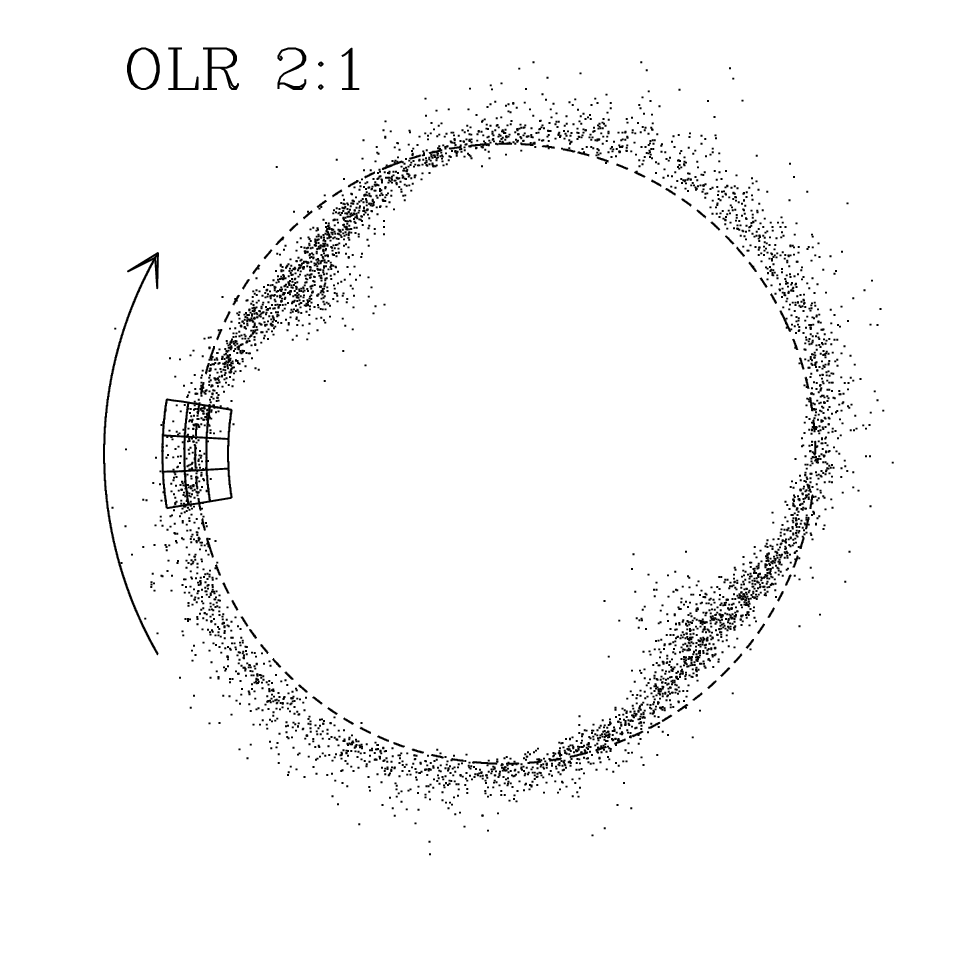
In Figure 3 we show the positions of stars associated with the Hyades in the Galactic plane for all models. Much as one would expect from the condition described by equation 2, the 4:1 resonances have groups of stars gathered at apocentre or pericentre at four different azimuths ( changing by as changes by ), producing a square or clover-leaf pattern in position in the Galactic plane. Similarly the 2:1 resonances have groups at apo- or peri-centre at two different azimuths ( changing by as changes by ), producing an oval pattern in position.
In Figure 3 we also show the position of the extended Solar neighbourhood which we will be investigating in velocity space to find the signature of the Hyades. The key thing to note is that the “stream” in position associated with the resonances runs in different directions near to the Sun, depending on whether they are inner or outer Lindblad resonances. ILRs produce streams that tend to be at in the immediate anti-rotation direction, and towards in the direction of rotation, whereas OLRs produce streams that are the other way around. Note that each case the Hyades stars in the Solar neighbourhood are all rotating in the same direction as the Galaxy and moving radially outwards, so they are not “following” the stream in the Galactocentric frame (though they are in the frame rotating with the perturbation).
These streams are of non-negligible width, controlled by the parameter in equation 9. It should be possible to determine the value of (or something similar, for a different model), as well the type of resonance, from observations by determining the range in (at a given ) over which the Hyades can be found (in velocity space). Sellwood (2010) attempted to estimate the time since the resonance occurred by comparing the width of the resonance in frequency to the width of the resonance in angle. That result is flawed because of the unrecognised impact of selection effects on the observed spread in angle, but determining the true value of would enable us to make an improved estimate. It should be noted that this can only be an upper estimate, without knowing the width in intrinsic in the libration of the resonantly trapped stars.


In Figure 5 we show the distribution in velocity space of stars associated with the Hyades in each model, separated into bins in the Galactic plane each of which covers in Galactocentric radius , in Galactocentric angle (corresponding to at the Solar radius), and only contains stars which are within of the Galactic plane. These bins are illustrated in Figure 4.
In Figure 5 the Hyades can clearly be seen as a strong feature in all three azimuthal bins at the Solar radius for all models. In each case the Hyades appear at a similar point in the plane as they do in the Solar neighbourhood. This is in keeping with the overdensity observed by A12. In bins at lower , the Hyades are found at higher , and in bins at higher , they are found at lower . This is because in all cases the Hyades are associated with a narrow range in angular momentum, which naturally produces a correlation between and . The peak of the distribution associated with the Hyades moves from in the inner bin to (varying slightly between the models). This is a somewhat smaller change than one would naively expect from angular momentum conservation given that the bin centres are apart, but this is because stars in the outer bins tend to be close to the central bin rather than spread evenly across the bin.
There are two notable differences between the ILR models and the OLR models. Probably the most useful difference, in terms of telling one model from another, is the variation in the number of stars associated with the Hyades in each spatial bin. The two ILR models tend to have many Hyades stars in the outer Galaxy, and few in the inner, in the direction of Galactic rotation and many in the inner Galaxy, and few in the outer, in the anti-rotation direction. The opposite is true in the case of the OLR models. This effect is most pronounced in the 4:1 resonances, with the 2:1 resonances placing few Hyades stars far from the Solar radius in this range of . This is because of the differences in the paths of the “streams” illustrated in Figure 3. The second difference is in the value of the peak in the velocity distribution in the inner or outer bins. The ILR models have a peak at in the bins and in the bins , whereas in the OLR models this is reversed, with for and for .
In Figure 6 we show the same figures for the model including the smooth background df. This shows that in the inner and outer bins with relatively strong signatures of the Hyades, we can expect to observe the Hyades above the background, but the weak signatures are lost in the background. It should be noted that this is, in some ways, a best case scenario, as we have assumed negligible uncertainty on velocity, a large number of observed stars (so shot noise doesn’t hide the Hyades) and ignore other substructure in the velocity diagram that might cause confusion (for example, from the dynamical structures associated with the Pleiades and Sirius moving groups).
We can look more closely at the distribution of stars in spatial bins similar to those used by A12. If we take a Galactocentric Cartesian coordinate system , with the Sun at , , and with increasing in the direction of Galactic rotation at the Sun, then we can take stars with , and in windows in the range to correspond to the areas probed by A12’s work (though they chose to take ). To probe the area in detail, while still using large spatial bins to maximise the numbers of stars per bin in a given survey, we consider overlapping bins. Each bin is wide in , and we consider bins with limits that are shifted by in from each other. These bins are illustrated in Figure 7.
In Figure 8 we show the distribution of stars in the space in each of these spatial bins. Again it is clear that the major difference between the various models is whereabouts in the Galaxy the Hyades remains a strong feature. Since these bins are in the anti-rotation direction from the Sun, the OLR models show a strong Hyades feature in the outer bins, and the ILR models show it in the inner bins.
Finally we look at the consequences of observational uncertainties on the structures observed in the plane for the various models. If we assume an uncertainty of in line-of-sight velocity, in proper motion, and per cent in distance (approximately the uncertainty on RAVE observations), and apply this to our models, we find the “observed” distribution in the plane shown in Figure 9. The most obvious consequence is that the entire velocity distribution gets stretched in the direction associated with the uncertainty in transverse velocity. This is because the dominant velocity uncertainty is that associated with the distance uncertainty. This uncertainty also weakens the signature of the Hyades in each case. The differences between the two models is discernible, but it is seriously faded. It is worth noting that the signatures of the ILR models are visible in the innermost spatial bin, but those of the OLR models are not in the outermost.
4.1 Comparison to observations
Isolating these signatures in real data is likely to be even harder than Figures 8& 9 would suggest, because there will be additional noise due to the relatively small number of stars that will have been observed in any given volume, and because the other stars will not be smoothly distributed in velocity space, but will be in various substructures, much as they are in the Solar neighbourhood. However, sophisticated analysis techniques such as wavelet transforms (A12 and references therein) may provide a means of finding even this weak signal in noisy, background dominated, data.
Currently available data, as analysed by A12, does show a feature consistent with any of these models at radii near . It is shown in their Fig. 3, second panel (labelled ), with the feature labelled “3” as it is the third greatest overdensity in the plot.
However, the panels showing the velocity distribution in bins at smaller or larger Galactocentric radii (labelled and respectively) do not show features that can be convincing associated with any of these models. The feature labeled “2” in the figure may appear to coincide with the overdensity expected from the ILR models shown here, but is at significantly higher ( faster than circular, as opposed to for the ILR models), and lacks the extension towards the left of the plot (i.e. towards higher positive ) that is a distinctive feature of all of these models (and the Hyades in the Solar neighbourhood). While there appears to be some small overdensity at the position that the OLR models would produce one in the figure, it is so minor that it is unlabelled, and is of completely the wrong shape (the feature labeled “4” in this figure is at much lower than one would expect for the Hyades and, as noted by A12, is almost certainly the Hercules stream).
A comparison of these models to figures showing the distribution of the overdensities in velocity space in more closely spaced, overlapping bins taken from the RAVE data (Antoja, priv. comm.) does not provide any significant further evidence for either the ILR or OLR models. Given the substantial impact of observational errors illustrated by Figure 9, and the further problems associated with low number statistics and a non-smooth background, this cannot reasonably be taken as evidence that these models are all wrong, but rather as an illustration that more accurate data will be required to determine which, if any, of these models is correct.


5 Conclusions
In this paper we have taken a detailed look at four different models for the Hyades, each of which accurately reproduce the signature of the Hyades moving group in the Solar neighbourhood, but which differ significantly from one another beyond it. The models represent stars trapped at four different resonances, and are produced using the torus fitting method to realize models described in angle-action variables.
We have shown that for each model we expect the Hyades to produce a significant overdensity in velocity space around the Solar radius, even from the Sun in Galactic azimuth. However this signature moves and fades with Galactocentric radius in a predictable way that provides a clear way of determining which kind of resonance is responsible. Most notably, if the Hyades are due to an ILR, they tend to be found at larger Galactocentric radii () in the direction of Galactic rotation, and smaller in the anti-rotation direction, whereas the opposite is true if they are due to an OLR.
It is worth noting that, as shown by Sellwood (2012), there are good theoretical reasons to expect trapping at an ILR, and it can be seen in simulations. It is not obvious that one should expect to see similar at an OLR, and neither trapping at the OLR or the ultra-harmonic resonance is observed in Sellwood’s simulations. An additional concern is that, as noted by Sellwood (2010), a significant spiral pattern with co-rotation around , as would be required to produce the Hyades through a 2:1 ILR, seems unlikely, which means that it would have to be due to some other perturbation, such as a rotating distortion of the halo. If the Hyades are the result of a an inner ultra-harmonic resonance with an perturbation (equivalent, in the models used in this paper, to a 4:1 ILR), this would be in keeping with the results of Siebert et al. (2012), who used model with a two arm spiral to explain a gradient in mean Galactocentric radial velocity found in RAVE data, and the model proposed to explain some elements of the local velocity distribution by Quillen & Minchev (2005). It should be noted that the absence of resonant trapping at the ultra-harmonic resonance in the simulations of Sellwood (2012) would seem to argue that if this is the result of resonance with a spiral with corotation at , the spiral would have to be 4-armed.
Presently available data (A12) suffers from low number statistics and uncertain distances, which leads to a significant uncertainty in the transverse velocity of the stars. This means we are not yet able to provide any significant extra insight as to which resonance is associated with the Hyades using observations from beyond the Solar neighbourhood.
With improved distance measurements and more observed stars, this situation will improve, and these easily tuneable models provided by the angle-action description of the phenomena will provide great insight into the nature of the resonance and, therefore, the perturbation to the Galaxy that is responsible.
Acknowledgments
We’re grateful to James Binney for a careful reading of a draft of this paper, and to Teresa Antoja for providing detailed figures of the velocity substructure found in the RAVE data. We thank the anonymous referee who provided a number of helpful suggestions and noticed one potentially terrible typographical error. This work is supported by a grant from the Science and Technology Facilities Council.
References
- Abazajian et al. (2009) Abazajian K. N., Adelman-McCarthy J. K., Agüeros M. A., et al., 2009, ApJS, 182, 543
- Antoja et al. (2011) Antoja T., Figueras F., Romero-Gómez M., Pichardo B., Valenzuela O., Moreno E., 2011, MNRAS, 418, 1423
- Antoja et al. (2012) Antoja T., Helmi A., Bienayme O., Bland-Hawthorn J., Famaey B., Freeman K., Gibson B. K., Gilmore G., Grebel E. K., Minchev I., Munari U., Navarro J., Parker Q., Reid W., Seabroke G. M., Siebert A., Siviero A., Steinmetz M., Williams M., Wyse R., Zwitter T., 2012, MNRAS, 426, L1
- Binney (2005) Binney J., 2005, in ESA Special Publication, Vol. 576, The Three-Dimensional Universe with Gaia, Turon C., O’Flaherty K. S., Perryman M. A. C., eds., p. 89
- Binney (2010) —, 2010, MNRAS, 401, 2318
- Binney (2012) —, 2012, MNRAS, 426, 1328
- Binney & McMillan (2011) Binney J., McMillan P., 2011, MNRAS, 413, 1889
- Binney & Tremaine (2008) Binney J., Tremaine S., 2008, Galactic Dynamics: Second Edition. Princeton University Press
- De Simone et al. (2004) De Simone R., Wu X., Tremaine S., 2004, MNRAS, 350, 627
- Dehnen (1998) Dehnen W., 1998, AJ, 115, 2384
- Dehnen (1999) —, 1999, ApJL, 524, L35
- Dehnen (2000) —, 2000, AJ, 119, 800
- Eggen (1996) Eggen O. J., 1996, AJ, 112, 1595
- ESA (1997) ESA, 1997, VizieR Online Data Catalog, 1239, 0
- Famaey et al. (2005) Famaey B., Jorissen A., Luri X., Mayor M., Udry S., Dejonghe H., Turon C., 2005, A&A, 430, 165
- Fux (2001) Fux R., 2001, A&A, 373, 511
- Hahn et al. (2011) Hahn C. H., Sellwood J. A., Pryor C., 2011, MNRAS, 418, 2459
- Helmi et al. (2006) Helmi A., Navarro J. F., Nordström B., Holmberg J., Abadi M. G., Steinmetz M., 2006, MNRAS, 365, 1309
- Holmberg et al. (2009) Holmberg J., Nordström B., Andersen J., 2009, A&A, 501, 941
- Kalnajs (1991) Kalnajs A. J., 1991, in Dynamics of Disc Galaxies, Sundelius B., ed., p. 323
- Kapteyn (1905) Kapteyn J. C., 1905, Reports of the British Association for the Advancement of Science, 257
- McMillan (2011a) McMillan P. J., 2011a, MNRAS, 414, 2446
- McMillan (2011b) —, 2011b, MNRAS, 418, 1565
- McMillan & Binney (2008) McMillan P. J., Binney J. J., 2008, MNRAS, 390, 429
- Minchev et al. (2010) Minchev I., Boily C., Siebert A., Bienayme O., 2010, MNRAS, 407, 2122
- Minchev et al. (2009) Minchev I., Quillen A. C., Williams M., Freeman K. C., Nordhaus J., Siebert A., Bienaymé O., 2009, MNRAS, 396, L56
- Navarro et al. (1996) Navarro J. F., Frenk C. S., White S. D. M., 1996, ApJ, 462, 563
- Pompéia et al. (2011) Pompéia L., Masseron T., Famaey B., van Eck S., Jorissen A., Minchev I., Siebert A., Sneden C., Lépine J. R. D., Siopis C., Gentile G., Dermine T., Pasquato E., van Winckel H., Waelkens C., Raskin G., Prins S., Pessemier W., Hensberge H., Frémat Y., Dumortier L., Bienaymé O., 2011, MNRAS, 415, 1138
- Quillen & Minchev (2005) Quillen A. C., Minchev I., 2005, AJ, 130, 576
- Quillen et al. (2009) Quillen A. C., Minchev I., Bland-Hawthorn J., Haywood M., 2009, MNRAS, 397, 1599
- Schönrich et al. (2010) Schönrich R., Binney J., Dehnen W., 2010, MNRAS, 403, 1829
- Sellwood (2010) Sellwood J. A., 2010, MNRAS, 409, 145
- Sellwood (2012) —, 2012, ApJ, 751, 44
- Siebert et al. (2012) Siebert A., Famaey B., Binney J., Burnett B., Faure C., Minchev I., Williams M. E. K., Bienaymé O., Bland-Hawthorn J., Boeche C., Gibson B. K., Grebel E. K., Helmi A., Just A., Munari U., Navarro J. F., Parker Q. A., Reid W. A., Seabroke G., Siviero A., Steinmetz M., Zwitter T., 2012, MNRAS, 425, 2335
- Steinmetz et al. (2006) Steinmetz M., Zwitter T., Siebert A., et al., 2006, AJ, 132, 1645