DCPT/13/04, IPPP/13/02
Emergence of the Electroweak Scale through the Higgs Portal
Abstract
Having discovered a candidate for the final piece of the Standard Model, the Higgs boson, the question remains why its vacuum expectation value and its mass are so much smaller than the Planck scale (or any other high scale of new physics). One elegant solution was provided by Coleman and Weinberg, where all mass scales are generated from dimensionless coupling constants via dimensional transmutation. However, the original Coleman-Weinberg scenario predicts a Higgs mass which is too light; it is parametrically suppressed compared to the mass of the vectors bosons, and hence is much lighter than the observed value. In this paper we argue that a mass scale, generated via the Coleman-Weinberg mechanism in a hidden sector and then transmitted to the Standard Model through a Higgs portal, can naturally explain the smallness of the electroweak scale compared to the UV cutoff scale, and at the same time be consistent with the observed value. We analyse the phenomenology of such a model in the context of present and future colliders and low energy measurements.
1 Introduction
The recent discovery of a particle which is likely to be the Higgs boson [1, 2, 3] with a mass of concludes the quest to complete the particle spectrum of the Standard Model. However, the Standard Model itself leaves many open questions. Most crucially, the question of the origin of the electroweak scale remains unanswered. Let us briefly consider the Higgs potential in the Standard Model,
| (1.1) |
for the Higgs doublet which in the unitary gauge takes the form . The minimum of the potential occurs at for negative and the mass of the Higgs boson is .
Choosing a value
| (1.2) |
for the Higgs mass parameter in (1.1), an expectation value for the Higgs field and the Higgs mass can be easily accommodated. However, the Standard Model itself cannot explain the value of this parameter and in particular its smallness compared to the UV cutoff, (which we take to be the scale of new physics in the UV where the Standard Model breaks down as an effective theory, e.g. ).
In a seminal paper [4] Coleman and Weinberg showed that in the absence of mass scales in the potential of a scalar field, a mass scale is nevertheless generated via dimensional transmutation from the running couplings, and indeed spontaneous symmetry breaking does occur. A minimal self-consistent theory for this mechanism at work is provided by massless scalar QED. This is a model with a massless complex scalar field11 1 We point out that we use the same normalisation as Coleman and Weinberg, treating the complex field as two real scalar fields with kinetic term .,
| (1.3) |
charged under a U(1) symmetry with gauge coupling . Starting from a classical potential and requiring that the renormalised mass term for vanishes, the authors of [4] find the 1-loop corrected potential
| (1.4) |
where is the renormalisation scale.
The essential feature/requirement employed here is that the renormalised mass at the origin in the field space is kept at zero,
| (1.5) |
In dimensional regularisation, which does not introduce any explicit scale aside from the RG scale, entering the logarithmically running couplings, this equation is satisfied automatically.22 2 No power-like divergencies proportional to the cutoff scale appear in dimensional regularisation, and in theories like ours, which contain no explicit mass scales at the outset, no finite corrections to dimensionful quantities can appear either. In other regularisation schemes such as e.g. the cutoff scheme, the zero on the right hand side of (1.5) corresponds to an exact cancellation of all the quadratically divergent parts between the bare mass squared terms and the counterterms.
The consequence of (1.5) is that no explicit mass scales are allowed in the effective potential of the theory, except the renormalisation scale appearing in the logarithm. This is the manifestation of the scale invariance of the classical massless theory; the scale invariance is broken only by the radiative corrections which introduce only a logarithmic scale dependence.
Now returning to the effective potential in (1.4), at small values of the field, the logarithm in the brackets always wins, giving the potential a downward slope. On the other hand, at values the slope is always positive. Accordingly we always have a minimum of the potential at a value . Using this, one can remove the renormalisation scale of the potential by renormalising at the acquired vacuum expectation value (vev) . Another simplification arises from the fact that if we choose the value of the -self-coupling squared at the minimum of the effective potential is negligible compared to the U(1) gauge coupling , as shown in Eq. (1.8) below, and we can drop the first term in brackets (1.4). We thus have
| (1.6) |
The minimum of the effective potential is at
| (1.7) |
and the vev is determined by the condition on the couplings renormalised at the scale of the vev [4],
| (1.8) |
The effective potential in the vacuum reads
| (1.9) |
Since the couplings run only logarithmically the vev fixed by the condition (1.8) depends exponentially on the coupling constants. In fact, in weakly coupled perturbation theory the vev is naturally generated at the scale which is exponentially smaller than the UV cutoff. This can be illustrated by solving the leading-order RG-running equation for the coupling ,
| (1.10) |
Upon integration and setting the RG scale we find
| (1.11) |
We see that the vev is generated at the scale which is exponentially smaller than the UV cutoff scale (in our case the Landau pole of ). Equation (1.11) is the consequence of the dimensional transmutation: the dimensionality of the vev is carried by the UV-scale Landau pole, while the exponential smallness of the ratio is guaranteed by the perturbativity of the coupling constant in the vacuum i.e. at the scale . This addresses the naturalness problem.
We would also like to quantify the exponential sensitivity of the vev to the input (or bare) values of the coupling constants at the UV cutoff scale (we continue calling it even though here we don’t think of it as a Landau pole). We proceed by solving the RG equation for the ratio of coupling constants, which is obtained by combining (1.10) with the RG equation for ,
| (1.12) |
For the ratio we find,
| (1.13) |
Upon integration and setting the RG scale and using the condition we obtain (we keep only the first term on the r.h.s. of (1.13))
| (1.14) |
This expression shows the exponential sensitivity of the vev to the values of the couplings at the UV cutoff. As a result, the vev can easily be made exponentially smaller than the UV cutoff (in agreement with what we have already concluded from (1.11)). Qualitatively the same behaviour holds beyond our simple approximation to the RG equations. This is shown in Fig. 1, where we show the ratio of at required to generate a hierarchy of 14, 15 or 16 orders of magnitude between and .
In summary, in a theory with no input mass scales, the Coleman-Weinberg (CW) mechanism generates a symmetry-breaking vev and the mass for the associated scalar from radiative corrections. These scales are natural in the sense that they are automatically exponentially suppressed compared to the UV scale at which we initialise the theory. Phenomenologically, however, this scenario has a fatal flaw: if is the Higgs, then the Higgs mass turns out to be too small. This is because the self-coupling is much smaller than the gauge coupling . From Eq. (1.9) one can calculate the physical mass of the Higgs remaining after spontaneous breaking of the gauge symmetry by shifting the field ,
| (1.15) |
In terms of the mass of the vector boson we have
| (1.16) |
This is in conflict with the observation that, in the Standard Model, the Higgs is heavier than the corresponding vector bosons.
To resolve this problem we thus need to look beyond the minimal Standard Model. In this paper we consider a very compact extension of the Standard Model where there is no longer a direct link between the Higgs mass and the SM vector boson masses, and consequentially, the Higgs can take its observed value GeV. At the same time, this formulation maintains the essential feature that all mass scales are generated radiatively through breaking of classical scale invariance via running couplings.
In the section 2 we outline the minimal model we want to study: a scale-invariant Standard Model with an additional CW “hidden sector” and the Higgs portal-type coupling to the SM. In section 4 we analyse the phenomenology of this model in the context of LHC and future colliders, and low energy measurements. We point out that with the Higgs mass now being a known quantity, the minimal model has only two remaining free parameters, and we show that the model is perfectly viable. The presently available Higgs data provide valuable constraints on the parameter space, while future experimental data on Higgs decays (as well as resonance searches) will further constrain model parameters, and will ultimately provide discovery potential for this model.
In a pre-LHC context this simple model has already been discussed in [5, 6] along with a variety of other similar scalar field models in [7, 8]. First model-building implications of a GeV Higgs have also been looked at in [9].
The use of the Coleman-Weinberg mechanism for BSM model building is motivated by and based on the concept of classical scale invariance. Although the scale invariance symmetry is anomalous, it has been argued in [10] that it may indeed be used as a model-building guide and to motivate Coleman-Weinberg type models [7]. In section 3 we provide another, renormalisation-group-inspired argument in favour of this model-building strategy.
Our conclusions are summarised in section 5.
2 Coleman-Weinberg with a Higgs portal
As we have seen in the previous section the main problem of the CW scenario is that the mass of the Higgs boson is too small within the SM. The reason is that the mass of the Higgs is directly linked to the mass of the gauge bosons and is 1-loop suppressed compared to those. A simple way to address this issue is to generate the mass scale in a “hidden sector” and then transmit it to the SM, where it directly acts as the scale of the pure SM. This breaks the direct CW relation between the SM gauge boson masses and the mass of the SM Higgs boson.
A simple model to realise this is a Higgs-portal model [11] with the CW toy model as a hidden sector [5, 6]. The classical potential for scalar fields is,
| (2.1) |
The first and the last terms are just the ordinary self-couplings for the Higgs field and field, while the second term is the Higgs-portal, coupling the SM Higgs field to the hidden sector field . For future convenience we chose the sign in front of this Higgs-portal coupling to be negative.
To check the stability of this potential we complete the square in (2.1)
| (2.2) |
The potential is then stable as long as
| (2.3) |
When the two sectors decouple.
For non-vanishing the Higgs portal interaction can generate the Higgs mass parameter of (1.1) via
| (2.4) |
Importantly, in Eq. (2.1) we have not allowed for any mass terms. In other words we have a completely scale-free potential even in presence of the Higgs portal coupling. We now proceed with employing the Coleman-Weinberg mechanism in the Higgs-portal theory (2.1) where the complex scalar is coupled as before to a U(1)hidden gauge theory (this forms the hidden sector), while the Higgs doublet has standard interactions with the SU(2)U(1) gauge fields (as well as matter fields) of the Standard Model. At the origin in field space, i.e. when all field vevs are zero, there are no scales present in the classical scale-invariant theory. We want to and can preserve this feature in the quantum-corrected full effective potential even after renormalisation by using33 3 The term vanishes by gauge invariance.
| (2.5) |
This is the same subtraction scheme as in the simple case (1.5), and as there, these conditions are automatic in dimensional regularisation of any theory with classical scale invariance. In other regularisation schemes one cancels quadratic divergencies between the bare masses and the counterterms. We elaborate on this in more detail in next section.
The easiest way to visualise the emergence of electroweak symmetry breaking in this theory is to consider a near decoupling limit. If we can essentially view the process of symmetry breaking independently in the two different sectors and we can view electroweak symmetry breaking effectively as a two step process.
In the first step the CW mechanism generates a (large44 4 Large compared to the electroweak scale of the standard model.) vev in the hidden sector through dimensional transmutation precisely as was outlined in the previous section. In the second step the vev is transmitted to the Standard Model via the Higgs portal, generating an effective mass parameter for the Higgs
| (2.6) |
Equation (1.2) dictates that fixes the electroweak scale, specifically,
| (2.7) |
This implies that when and also is much smaller than other SM Higgs couplings, the electroweak scale is suppressed compared to the hidden sector scale, as was anticipated,
| (2.8) |
The fact that the generated electroweak scale is much smaller than guarantees that any back reaction on the hidden sector vev is negligible.
Let us now verify that the dimensional transmutation phenomenon continues to work in our more complicated theory and all the required vevs are natural. To see this we start from the Higgs-portal effective potential
| (2.9) |
Here we are keeping 1-loop corrections arising from interactions of with the U(1) gauge bosons in the hidden sector, but neglecting radiative corrections from the Standard Model sector. The latter would produce only subleading corrections to the vevs. The -minimisation condition55 5 Minimisation with respect to does not give anything new beyond the known SM condition (1.2). for this effective potential is (cf. (1.7) and (2.8))
| (2.10) |
We thus conclude that the dimensional transmutation continues to work and the and the vev is determined by the condition on the four couplings renormalised at the scale of the vev
| (2.11) |
For small , this is a small deformation of the original condition (2.11). In the near-decoupling case of we are interested here, the modifications are negligible. But even in a more general case, there are no obstructions for the Coleman-Weinberg mechanism to work.
The two vevs, and are generated naturally through dimensional transmutation in our framework similarly to (1.11),
| (2.12) |
Since massive vector bosons of the Standard Model play no role in stabilising the minimum of the Coleman-Weinberg potential in our Higgs portal model, there is no condition linking the SM gauge and the Higgs couplings. As a result the vector boson masses and the Higgs boson mass are independent and can take their observed SM values.
3 Arguments in favour of vanishing mass terms at the origin of the potential
The exponential sensitivity of the Higgs vacuum expectation value to the boundary values of the couplings, and the natural generation of the hierarchy between the EWSB scale and cut-off scale in (2.12), crucially depend on the choice of massless renormalisation conditions Eq. (2.5) at the origin of the field space. In this section we want to give arguments in favour of this choice.
A suitable symmetry to forbid mass terms for scalars is scale invariance. Indeed, in absence of scale invariance the classical potential Eq. (2.1) would allow for two additional mass terms,
| (3.1) |
In the class of theories we consider, scale invariance is a classical symmetry which is broken by quantum corrections, specifically by the logarithmic running of the couplings. One might therefore query if it is allowed to set these mass terms to zero in full quantum theory, as we have done in Eq. (2.5). In [10, 7] this question has been answered favourably based on the special role played by dimensional regularisation and considering the anomaly in the trace of the energy-momentum tensor. Here, we provide additional perspective and support based on the renormalisation group, and also address the question of scheme dependence.
First we want to check if our requirement that the mass terms vanish (2.5), is affected by a change in the renormalisation scale. To do this we can look at the appropriate renormalisation group equations for the mass terms. In dimensional regularisation they have the form,
| (3.2) |
with and the anomalous dimension of the Higgs and field respectively, and as before.
We can clearly see that is a fixed point of the RG evolution and, once enforced at one scale, it holds at all scales. In this sense – within dimensional regularisation – our renormalisation conditions Eq. (2.5) are self-consistent and contain no fine-tuning. They correspond to an enhanced unbroken symmetry for these couplings.
In the argument above we made use of a specific regularisation scheme: dimensional regularisation. In other regularisation schemes66 6 Most other schemes introduce a new mass scale which explicitly breaks scale-invariance. the (one-loop) RG equations have a different form,
| (3.3) |
with constants that depend on the regularisation scheme.
The terms destroy the fixed point at . Instead we now have a partial77 7 I.e. it is a fixed point when we neglect the running of , and . fixed point at,
| (3.4) |
Neglecting the evolution of , and we can now write the RG equation for as
| (3.5) |
This equation has the simple solution,
| (3.6) |
where the staring point for the trajectory is , so that the combination appearing above, is . We now let the trajectory run from the high scale to a low value of . At weak coupling we can neglect the anomalous dimensions. Using an initial value corresponding to a vanishing mass at the scale we recover the usual quadratic divergencies,
| (3.7) |
In all regularisation schemes with non-vanishing , scale invariance is broken more strongly than in dimensional regularisation. We can therefore turn the argument around and argue that dimensional regularisation, having no quadratic divergencies, is the scheme which exhibits the smallest breaking of scale invariance. If we now insist that scale invariance is broken minimally by quantum corrections we are automatically led to dimensional regularisation and therefore Eq. (3.2) and consequently to our renormalisation conditions Eq. (2.5).
In absence of additional mass scales in the theory we are free to make this choice. Indeed one can argue that this is a preferred choice since in this case the only scale invariance breaking effect is the logarithmic running of the dimensionless couplings, which is independent of the regularisation scheme. All scheme-dependent (and therefore unphysical) effects are set to zero.
Let us take a step back from our concrete model and take a look at the more general situation. From a renormalisation group point of view, consistent theories are those that have a UV fixed point in the space of dimensionless coupling constants (all coupling constants of higher dimensional operators can be made dimensionless by scaling with an appropriate power of the RG scale, therefore this space is very infinite dimensional). In order for a theory to be predictive we need to be able to describe it by a finite number of parameters. For the UV fixed point this means the following: the space of all RG trajectories ending in the fixed point as the RG scale is taken to infinity is finite dimensional. The number of these dimensions is the number of free parameters. In the usual language these are the relevant parameters. Exciting a combination of coupling constants that is not in this subspace leads to an RG trajectory that (per definition) does not end in the fixed point as we go into the UV and the theory has incurable divergencies. The fixed point of a theory defined in this manner can be in the perturbative region where all coupling constants are small, but it can also be in a non-perturbative regime. In the latter case we have a non-perturbatively renormalisable theory in the sense of Weinberg’s scenario of “asymptotic safety” [12].
To give a concrete example, consider QCD with one flavour of massive fermions. This theory has two relevant parameters that can be chosen to be non-vanishing, the gauge coupling constant and the mass divided by the RG scale , . The RG equations are
| (3.8) |
One can easily check that starting from any (sufficiently small) value of and , we end up in the UV fixed point . However, for any “non-renormalisable” operator such as, e.g., with dimensionless coupling constant, we have,
| (3.9) |
which for any starting point with non-vanishing (but still close enough to the fixed point) has a trajectory that rapidly moves away from the fixed point. The same argument holds for any other higher dimensional operator.
The terms on the right hand sides of Eqs. (3.8), (3.9) that are linear in the couplings whose change is described on the left hand sides, describe the approach to, or running away from the fixed point in the UV88 8 More precisely the are the eigenvalues of the stability matrix of the system of RG equations. Close to the perturbative fixed points, they are given by minus the naive dimension of the coupling plus its anomalous dimension.,
| (3.10) |
Clearly, those directions with negative , approach the fixed point as the RG-scale goes to infinity; while those with positive , diverge. The case with leads to the usual marginal behaviour with logarithmic running towards (or away from) the fixed point.
Going in the opposite direction towards smaller , the operators with are exactly those that quickly obtain very large values. This is where the hierarchy problem lies. Choosing “natural” initial values for those operators at some UV scale, we get enormous values at a smaller scale. Vice versa, to get a value at some small scale requires us to finely tune the initial value at the high scale to be extremely small.
Importantly the are the critical exponents of the theory which are thought to be scheme-independent.
Our proposal is now as follows. Let us restrict our theory to live on a subspace of all trajectories which end in the fixed point. This subspace is defined by only exciting the marginal trajectories. Then all scales are generated via dimensional transmutation from the logarithmic running of the coupling constants. This is not a fine-tuning because we require the operators to be exactly zero, i.e. we are living exactly on this well-defined subspace99 9 While the precise shape of this subspace is scheme dependent, its existence and dimensionality is not..
Our concrete example now shows that we can choose the initial value of the Higgs mass operator at the high scale to be vanishing while still getting a phenomenologically viable non-vanishing vacuum expectation value (and physical Higgs mass) by dimensional transmutation from the marginal operators which exhibit only logarithmic running.1010 10 There is a beauty defect in our theory in that the marginal couplings are actually marginally irrelevant, but one can hope to cure this by a suitable embedding in a more complete theory. The trajectories in the subspace requiring all , are exactly those that correspond to classical scale invariance, broken only by the logarithmic running induced by quantum corrections.
Alternatively one can consider theoretical setups like Supersymmetry (SUSY) where the quadratic divergences are absent1111 11 One could be even more ambitious and ask that the theory is finite but this does not change our argument.. Such a theory has an additional scale (SUSY-breaking scale) above which the quadratic divergencies are canceled. This scale is physical in the sense that the dynamics of the theory above this scale is qualitatively different from the behaviour in the IR. This is for example due to the appearance of new degrees of freedom at higher energies. In such a situation we get finite threshold corrections from these additional degrees of freedom in any regularisation scheme. Simulating the quadratic divergencies of ordinary theories, these threshold corrections typically also scale quadratically with the scale of new physics. In the case of SUSY, above the SUSY-breaking scale quadratic divergences are canceled between bosons and fermions, leaving threshold corrections to the Higgs mass. These corrections are proportional to the mass squares of the SUSY partners of the SM particles and therefore quadratically sensitive to the scale at which SUSY is broken.
Even in this type of setup, our Coleman-Weinberg scenario is a helpful step to bridge the (possibly large) gap to this scale of new physics without generating a big fine-tuning. In the more complete theory we then only need to ensure that the sum total of all the finite threshold corrections vanishes. To us this seems a more achievable goal then getting a small (compared to the scale of new physics) but non-vanishing sum of threshold corrections.
4 Phenomenology
Let us investigate in this section the phenomenological viability as well as possible signatures of the proposed model.
In the hidden sector we have two additional fields and the extra U(1)hidden gauge field . After acquires a non-vanishing vev the gauge field becomes massive with a mass
| (4.1) |
In principle this extra U(1)hidden gauge boson can kinetically mix [13] with the hypercharge U(1), allowing for a rich phenomenology which can also be tested at the LHC [14]. Here we will not consider such a mixing and instead focus only on those interactions that must be present in order to ensure a working electroweak symmetry breaking, which will also modify the Higgs phenomenology.
In absence of kinetic mixing the dominant interaction between the hidden sector and the SM is via the Higgs portal coupling . The lowest order effect arises from the mixing between the SM Higgs and the hidden Higgs . The two scalars, and , mix via the mass matrix,
| (4.2) |
with the mixing parameter,
| (4.3) |
and the masses
| (4.4) |
These are the same as we had in the decoupled case () for the Higgs mass and the CW scalar mass.
In Eq. (4.2) we have also included one-loop corrections to the SM Higgs mass,
| (4.5) |
Numerically, these corrections are dominated by the top-quark loop and are therefore negative. While the resulting contributions are small for the nearly decoupled limit and at large , they lead to interesting effects for the case of small and moderate Higgs portal coupling.
Depending on the CW mass scale induced in the hidden sector, the model predicts new resonant structures in di-Higgs analysis or a hidden Higgs decay phenomenology as main modifications of the electroweak sector compared to the SM.
This matrix can be easily diagonalised with a rotation,
| (4.6) |
where the right hand side in the definition of gives in the case of small mixing.
Up to order (i.e. to leading order in ) the masses of the two eigenstates are simply
| (4.7) |
Fixing the (dominantly SM like) state to have a mass of we can now look at possible constraints on the only two remaining parameters: the mixing angle , and the mass of the second eigenstate. Due to the rotation (4.6) the model will show the character traits of a Higgs portal model [11, 15, 16, 17, 18], however with restrictions on the parameters that follow from transmitting EWSB to the visible sector as laid out in the previous sections.
Let us enumerate the parameters of our model in the small regime we are working in. The SM Higgs self-coupling is fixed by the ratio of known electroweak scales, while the other self-coupling, , is determined from the CW dimensional transmutation condition:
| (4.8) |
There are two undetermined parameters in our model which one can take to be the hidden sector gauge coupling, , and the (small) portal coupling . In this case, the two mass scales associated with the hidden scalar are fixed,
| (4.9) |
and the hidden sector vector mass is given by
| (4.10) |
Alternatively, the two free parameters can be chosen to be the mass of the hidden Higgs, , and the Higgs portal coupling . In this case, gauge coupling (and the mixing ) is determined via
| (4.11) |
In analogy to the Standard Model sector one may expect be of order but it could also be much smaller (cf. the hyperweak interactions in [19]). In the latter case one would, however, also need to explain an incredibly small . More importantly, for small it is crucial to take into account higher order corrections to Eq. (4.7),
| (4.12) |
As the SM model correction is negative (and quite sizeable) this enforces a minimal value for from the stability requirement ,
| (4.13) |
The minimal mass for can also be translated into a minimal value for
| (4.14) |
and, more importantly, into the lower bound for the mass of the U(1)hidden gauge boson,
| (4.15) |
For the physical mass Eqs. (4.12) and (4.13) also entail that values much below require some amount of fine-tuning as it involves a cancellation between and the SM correction. Moreover, for very small hidden Higgs masses the mixing is very strongly constrained from fifth force measurements [20]. In the following we will therefore mostly concentrate on the case of moderate and hidden Higgses with masses .
A first constraint can be imposed from theoretical reasoning. From Eq. (2.11) we can see that grows as and/or are increased raising the possibility of a nearby Landau Pole. Requiring that there is no Landau pole in for at least a few orders of magnitude puts already fairly strict limits on both and . Neglecting the contribution to the running of the solutions to the RG equations are given in [4]. In Fig. 2 we show the constraints arising from a hierarchy of 4 and 16 orders of magnitude between and the Landau pole yellow and light green, respectively. We can see that this automatically restricts us to fairly small . The used approximation is conservative in the sense that the contribution to the running of is positive speeding up the approach to the Landau pole. On the other hand for small the neglected term quickly becomes very small.
If the mass the ordinary Higgs can decay into two hidden Higgses. In leading order in the mixing angle this decay occurs via the term
| (4.16) |
and the SM-like Higgs trilinear interaction. The rotation to the physical mass eigenstates complicates the formulea, i.e. the trilinear couplings get more involved (see e.g. Refs. [15, 21] for detailed discussion). We fully include these nonlinear effects in our later scan but only sketch the line of thought in the following which is valid for small mixing, i.e . Hence, the dominant part of the corresponding partial decay width is
| (4.17) |
and needs to be taken into account for the Higgs modified branching ratios (BRs). A similar equation holds for with and . In our simple setup there are no light hidden sector particles into which the hidden Higgs can decay. The therefore decays back into SM particles via the mixing with the Higgs and its couplings to light particles. The branching ratios are the same as for the SM Higgs with mass , but the width, as well as the production cross sections from visible matter, are reduced by a factor ,
| (4.18) | ||||
| (4.19) |
Note, that already the SM Higgs decay width is quite small, [22] and decreases more or less linearly (until the bottom threshold is crossed) with the mass. Combining this with a small mixing angle, becomes an extremely narrow resonance. Indeed for very small values of we may even have displaced vertices or can use adapted trigger strategies [23] to constrain such a scenario at the LHC (signatures of this type have been described in [24]).
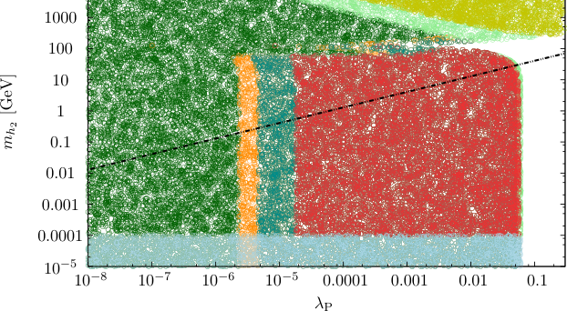
In Fig. 2 we show the results of a parameter scan projected on the plane (we identify ). We include constraints from current LHC searches for the mass range , which can be as low as [25] and the LEP constraints for , precision constraints from the parameters [26] as well as tree-level unitarity constraints are imposed. The currently allowed coupling span of the Higgs measurements is at 1 sigma [27], which is the combined result of the discovery channels . In our model we always have due to mixing; a statistically significant measurement of the enhancement in the would therefore be at odds with the most straightforward implementation of EWSB as described in the preceding sections.
A significant decay of the Higgs candidate into fermions is yet to be measured. Current constraints on (with SM branching ratio ) follow from biasing the coupling fit with the SM assumption of a total SM-like Higgs decay width. The observed rates, at the current precision can be understood as a limit on the total Higgs width itself. Given that we have a potentially large coupling to a new decay channel at a large available phase space Eq. (4.17) an upper limit on the total Higgs width constrains the model. Recent analyses suggest [28] and we include this bound to our scan. We also display the improvement of the ruled-out region due to the combination of a high-luminosity LHC run in combination with a linear collider on the basis of the most recent coupling fits of Ref. [29]. Note that, other than at a hadron collider, the total Higgs width can be measured by correlating Higgs production in weak boson fusion and the decay at the level [30, 16].
From Fig. 2 we see that there is a large parameter region of the model allowed by current measurements (note that the allowed region, of course further extends to smaller and also to larger masses). The model can be efficiently constrained by measuring the Higgs candidates cross section and decay width as precisely as possible, which can be done extraordinarily well at a precision collider instrument such as a future linear collider. The small funnel region at around follows from relaxed bounds and kinematic suppersion in the vicinity of the Higgs candiadate. within this range is then unconstrained more or less irrespective of the precise value of .
Since, is small by consistency and RG arguments, we face small mixing with the hidden sector which effectively yields a phenomenologically decoupled Higgs partner in the single Higgs channels of [2, 3] when background uncertainties are taken into account. When the mixing is rather larger sensitivity in SM-like Higgs searches can provide powerful means to constrain the model for heavy . Given the small width, standard analyses can be straightforwardly extended beyond the current upper limit of .
The small mixing make electroweak precision constraints (which can be straightforwardly generalised to observables beyond and flavour constraints in the present model) redundant: The region excluded by the current ellipse corresponds to large mixing , a region which is well excluded by RG arguments. In this sense, electroweak precision does not yield an additional constraint, but is implied by the consistency of the model itself.
The suppression of single- phenomenology can in principle be counteracted in the di-Higgs channels (see e.g. Ref. [31] for an example in a different context). The resonance is extremely narrow, and for the parameter space it naturally appears in the TeV regime. Such signatures have been investigated in [32, 21]. While the small mixing angle naively means a suppressed -channel contribution of to the di-Higgs phenomenology, it exclusively decays to a SM-like di-Higgs system in our setting with a potentially large coupling GeV. The small coupling of to the top quarks running in the gluon fusion loops however can typically not be beaten by the vertex. This contribution has to be put in contrast to the off-shell vertex which is SM-like and, more importantly for high energetic Higgses, to the box-induced continuum production. We have performed a full one-loop computation of via gluon fusion (which by far the most dominant production mode in the SM) in the proposed model and have scanned the cross section for a couple of parameter points and always find a di-Higgs cross section of fb. This agrees with the tree-level SM result [33] within uncertainties and we expect that adapting SM Higgs-like searches for the heavy is going to result in more solid constraints earlier.
In total, precision analyses of the Higgs-like candidate at 125 GeV and extending Higgs boson-like searches beyond therefore provide the best handles to constrain this model in its simplest implementation. The portal parameter, which is required to be small in the limit of light can be efficiently constrained by measuring the couplings at a future linear collider. Excluding heavy fields in high luminosity LHC searches limit the parameter space for .
Low energy measurements on the other hand are highly sensitive to very light masses, e.g. fifth force measurements can probe mixing angles for [20], which limits the model for such very small combinations. For moderate masses stellar evolution sets strong constraints on scalar couplings to two photons [34]. The coupling of to two photons is given by,
| (4.20) |
we can translate these bounds into a limit on for masses .
5 Conclusions
The Coleman-Weinberg mechanism is an intriguing possibility to naturally generate a very small scale. However, if done within the Standard Model its main prediction of a very light Higgs (far below the -mass) is in clear conflict with the experimental observation of a Higgs(-like) particle at 125 GeV. In this paper we have shown that a simple Higgs-portal model allows to generate the electroweak scale via the Coleman-Weinberg mechanism while at the same time giving a phenomenologically viable Higgs mass. The simple model we have discussed has a rich phenomenology and can be tested at the LHC.
While the explicit model considered in this paper is interesting on its own right thanks to its simplicity, it can also be viewed as a representative of a whole class of models in which the Coleman-Weinberg mechanism generates a low scale in the hidden sector which then is transmitted to the SM via the Higgs portal.
An essential requirement for the Coleman-Weinberg mechanism to work is that the renormalised mass at the origin of the potential vanishes. All scales are then generated from dimensional transmutation and are exponentially suppressed compared to the UV scale at which the theory is initialised. We have collected and discussed various arguments why the vanishing of the renormalised mass terms is a sensible condition. We find two main possibilities.
- 1.
Let us take the full classical theory to be massless and scale invariant. Scale invariance is broken in the quantum theory. Dimensional regularisation is the scheme which (to our knowledge) breaks scale invariance minimally. In dimensional regularisation the condition of vanishing masses at the origin is independent of the renormalisation scale and can therefore be imposed consistently without fine-tuning (in a more general scheme a similar condition can be defined consistently). The radiative generation of the EWSB scale in the full theory then proceeds via the CW mechanism as described in the body of the paper.
- 2.
Alternatively, assume that only the low energy theory we observe, has approximate scale invariance up to quantum corrections. The scale invariance breaking effects of additional high scale physics cancels exactly (not approximately as one would require to generate a small renormalised mass scale at the origin of field space).
The model’s phenomenology is that of a Higgs portal model, however with constraints imposed that arise from generating the electroweak scale via a small visible-hidden sector coupling. The modifications compared to the SM are generically small, and exclusion bounds are driven by precision investigations of the Higgs boson candidate. In essence, electroweak symmetry breaking proceeds along the lines of the SM, with modifications only due to small mixing effects and total Higgs width modifications. All these quantities can be determined most precisely at a future linear collider.
Although our simple setup cannot be considered a full solution to the hierarchy problem it provides a simple and experimentally testable scenario that may act as a first step to gain additional insight on the mechanism that generates the electroweak scale.
Acknowledgements
We would like to thank A. Hebecker, J. Pawlowski, J. Redondo, T. Plehn, B. Stech and C. Wetterich for helpful and stimulating discussions. CE acknowledges funding by the Durham International Junior Research Fellowship scheme. VVK gratefully acknowledges the support of the Wolfson Foundation and the Royal Society.
References
- [1] F. Englert and R. Brout, Phys. Rev. Lett. 13 (1964) 321, P. W. Higgs, Phys. Lett. 12 (1964) 132 and Phys. Rev. Lett. 13 (1964) 508, G. S. Guralnik, C. R. Hagen and T. W. B. Kibble, Phys. Rev. Lett. 13 (1964) 585.
- [2] G. Aad et al. [ATLAS Collaboration], Phys. Lett. B 716 (2012) 1.
- [3] S. Chatrchyan et al. [CMS Collaboration], Phys. Lett. B 716 (2012) 30.
- [4] S. R. Coleman and E. J. Weinberg, Phys. Rev. D 7 (1973) 1888.
- [5] R. Hempfling, Phys. Lett. B 379 (1996) 153.
- [6] W. -F. Chang, J. N. Ng and J. M. S. Wu, Phys. Rev. D 75 (2007) 115016.
- [7] K. A. Meissner and H. Nicolai, Phys. Lett. B 648 (2007) 312, Phys. Lett. B 660 (2008) 260.
- [8] R. Foot, A. Kobakhidze and R. R. Volkas, Phys. Lett. B 655 (2007) 156, R. Foot, A. Kobakhidze, K. .L. McDonald and R. .R. Volkas, Phys. Rev. D 76 (2007) 075014, Phys. Rev. D 77 (2008) 035006, S. Iso, N. Okada and Y. Orikasa, Phys. Lett. B 676 (2009) 81, M. Holthausen, M. Lindner and M. A. Schmidt, Phys. Rev. D 82 (2010) 055002, R. Foot, A. Kobakhidze and R. R. Volkas, Phys. Rev. D 82 (2010) 035005, L. Alexander-Nunneley and A. Pilaftsis, JHEP 1009 (2010) 021.
- [9] S. Iso and Y. Orikasa, arXiv:1210.2848 [hep-ph].
- [10] W. A. Bardeen, FERMILAB-CONF-95-391-T.
- [11] for early work see e.g. T. Binoth and J. J. van der Bij, Z. Phys. C 75, 17 (1997), R. Schabinger and J. D. Wells, Phys. Rev. D 72 (2005) 093007, B. Patt and F. Wilczek, arXiv:hep-ph/0605188.
- [12] S. Weinberg, in General Relativity: An Einstein centenary survey, Eds. S.W. Hawking and W. Israel, Cambridge University Press (1979), p. 790.
- [13] L. B. Okun, Sov. Phys. JETP 56 (1982) 502 [Zh. Eksp. Teor. Fiz. 83 (1982) 892], B. Holdom, Phys. Lett. B 166, 196 (1986).
- [14] M. T. Frandsen, F. Kahlhoefer, A. Preston, S. Sarkar and K. Schmidt-Hoberg, JHEP 1207 (2012) 123, S. Chatrchyan et al. [CMS Collaboration], Phys. Lett. B 714 (2012) 158, J. Jaeckel, M. Jankowiak and M. Spannowsky, arXiv:1212.3620 [hep-ph].
- [15] S. Bock, R. Lafaye, T. Plehn, M. Rauch, D. Zerwas and P. M. Zerwas, Phys. Lett. B 694 (2010) 44, C. Englert, T. Plehn, D. Zerwas and P. M. Zerwas, Phys. Lett. B 703 (2011) 298.
- [16] C. Englert, T. Plehn, M. Rauch, D. Zerwas and P. M. Zerwas, Phys. Lett. B 707 (2012) 512, J. H. Collins and J. D. Wells, arXiv:1210.0205 [hep-ph].
- [17] J. R. Espinosa, M. Muhlleitner, C. Grojean and M. Trott, JHEP 1209 (2012) 126.
- [18] E. Weihs and J. Zurita, JHEP 1202 (2012) 041, D. Bertolini and M. McCullough, JHEP 1212 (2012) 118, B. Batell, D. McKeen and M. Pospelov, JHEP 1210 (2012) 104.
- [19] C. P. Burgess, J. P. Conlon, L-Y. Hung, C. H. Kom, A. Maharana and F. Quevedo, JHEP 0807 (2008) 073.
- [20] M. Ahlers, J. Jaeckel, J. Redondo and A. Ringwald, Phys. Rev. D 78 (2008) 075005.
- [21] M. J. Dolan, C. Englert and M. Spannowsky, arXiv:1210.8166 [hep-ph].
- [22] A. Djouadi, J. Kalinowski and M. Spira, Comput. Phys. Commun. 108 (1998) 56, A. Bredenstein, A. Denner, S. Dittmaier and M. M. Weber, Phys. Rev. D 74 (2006) 013004.
- [23] G. Ciapetti, ATL-COM-PHYS-2008-155, A. Nisati, S. Petrarca, G. Salvini, ATL-MUON-97-205, S. Ambrosanio, B. Mele, S. Petrarca, G. Polesello, A. Rimoldi, ATL-PHYS-2002-006, S. Tarem et al., ATL-PHYS-PUB-2005.022, J. Ellis, A.R. Raklev, O.K. Oye, ATL-PHYS-PUB-2007-016, S. Tarem, S. Bressler, H. Nomoto, A. Di Mattia, ATL-PHYS-PUB-2008-01.
- [24] C. Englert, T. Plehn, D. Zerwas and P. M. Zerwas, Phys. Lett. B 703 (2011) 298.
- [25] The ATLAS collaboration, ATLAS-CONF-2012-170, The CMS collaboration, CMS-PAS-HIG-12-045.
- [26] M. E. Peskin and T. Takeuchi, Phys. Rev. Lett. 65 (1990) 964, M. E. Peskin and T. Takeuchi, Phys. Rev. D 46 (1992) 381.
- [27] A. Azatov, R. Contino and J. Galloway, JHEP 1204 (2012) 127, D. Carmi, A. Falkowski, E. Kuflik, T. Volansky and J. Zupan, JHEP 1210 (2012) 196, P. P. Giardino, K. Kannike, M. Raidal and A. Strumia, Phys. Lett. B 718 (2012) 469, J. Ellis and T. You, JHEP 1209 (2012) 123, J. R. Espinosa, C. Grojean, M. Muhlleitner and M. Trott, JHEP 1212 (2012) 045, T. Plehn and M. Rauch, Europhys. Lett. 100, 11002 (2012), T. Corbett, O. J. P. Eboli, J. Gonzalez-Fraile and M. C. Gonzalez-Garcia, arXiv:1211.4580 [hep-ph], E. Masso and V. Sanz, arXiv:1211.1320 [hep-ph].
- [28] B. A. Dobrescu and J. D. Lykken, arXiv:1210.3342 [hep-ph].
- [29] M. Klute, R. Lafaye, T. Plehn, M. Rauch and D. Zerwas, arXiv:1301.1322 [hep-ph].
- [30] C. F. Duerig, Master thesis, University Bonn (2012), http://lhc-ilc.physik.uni-bonn.de/thesis/Masterarbeitduerig.pdf
- [31] B. A. Dobrescu, G. D. Kribs and A. Martin, Phys. Rev. D 85 (2012) 074031, G. D. Kribs and A. Martin, Phys. Rev. D 86 (2012) 095023.
- [32] M. Bowen, Y. Cui and J. D. Wells, JHEP 0703 (2007) 036.
- [33] T. Plehn, M. Spira and P. M. Zerwas, Nucl. Phys. B 479 (1996) 46 [Erratum-ibid. B 531 (1998) 655], see also M. Spira, Hpair, http://people.web.psi.ch/spira/proglist.html.
- [34] G. G. Raffelt, D. S. P. Dearborn, Phys. Rev. D36 (1987) 2211, Phys. Rev. D 37 (1988) 549, G. G. Raffelt, G. D. Starkman, Phys. Rev. D40 (1989) 942, G. G. Raffelt, “Stars as laboratories for fundamental physics: The astrophysics of neutrinos, axions, and other weakly interacting particles”, Chicago, USA: Univ. Pr. (1996) 664 p.