跳到论文正文
W Papers独立论文阅读器 arXiv:1301.4199 论文正文 计算阅读时间 · 0%
引用这篇论文根据当前论文元数据生成,正式投稿前建议核对。


License: arXiv.org perpetual non-exclusive license
arXiv:1301.4199v1 [math-ph] 17 Jan 2013

Multichannel generalization of eigen-phase preserving supersymmetric transformations

Andrey M Pupasov-Maksimov Email: pupasov@phys.tsu.ru Affiliation: OOO Expert Energo, Moscow, Russia
Abstract

We generalize eigen-phase preserving (EPP) supersymmetric (SUSY) transformations to N>2N>2 channel Schrödinger equation with equal thresholds. It is established that EPP SUSY transformations exist only in the case of even number of channels, N=2​MN=2M. A single EPP SUSY transformation provides an M⁡(M−1)+2M(M-1)+2 parametric deformation of the matrix Hamiltonian without affecting eigen-phase shifts of the scattering matrix.

August 24, 2026

1 Introduction

In this paper we study NN channel radial Schrödinger equation with equal thresholds. Such equation may describe scattering of particles with internal structure, for instance, spin [1, 2, 3]. Supersymmetric (SUSY) transformations allow analytical studies of Schrödinger equation with a wide class of interaction potentials [4, 5, 6, 2]. In particular, the inverse scattering problem [8, 9] for two-channel Schrödinger equation with equal thresholds may be treated by combined usage of single channel SUSY transformations [10] and eigen-phase preserving (EPP) supersymmetric (SUSY) transformations [11]. These transformations conserve the eigenvalues of the scattering matrix and modify its eigenvectors (coupling between channels), in a contrast to phase-equivalent SUSY transformations which do not modify scattering matrix at all [12, 13, 14, 15].

In [3] the two-channel neutron-proton potential was reproduced by a chain of SUSY transformations, where the coupled channel inverse scattering problem were decomposed into the fitting of the channel phase shifts [10, 16] and the fitting of the mixing between channels. The fitting of the mixing between channels was provided by the EPP SUSY transformations.

This paper extends the two-channel EPP SUSY transformations to higher number of channels.

The paper is organized as follows. We first fix our notations and recall basics of SUSY transformations [6, 17, 18, 19]. Given the explicit form of a second-order SUSY transformation operator we study the physical sector of SUSY transformations between real and symmetric Hamiltonians. We analyze the most general form of a second-order SUSY transformation for the case of mutually conjugated factorization energies. Then we discuss applications of SUSY transformations to the scattering problems and calculate how SS-matrix transforms.

We start section 3 re-examining the conservation of its eigenvalues in the two-channel case. There is the following asymptotic condition for EPP SUSY transformations. The term with first-order derivative in the operator of EPP SUSY transformation vanishes at large distances.

To generalize EPP SUSY for arbitrary number of channels we study the matrix equation which comes from this asymptotic condition. We find that EPP SUSY transformations may exist for 2​M2M-channels only and obtain their general form. A 4-channel example explicitly shows how EPP SUSY transformations acts. We conclude with a summary of the obtained results and discussions of possible applications.

2 Second order SUSY transformations

2.1 Definition of SUSY transformations

SUSY transformations of stationary matrix Schrödinger equation are well known [17, 19]. In this subsection we just fix our notations.

Consider a family of matrix Hamiltonians ℍ={Ha}\mathbb{H}=\{H_{a}\}

Ha=−IN​d2d​r2+Va​(r),H_{a}=-I_{N}\frac{d^{2}}{dr^{2}}+V_{a}(r)\,, (1)

where INI_{N} is the N×NN\times N identity matrix, Va​(r)V_{a}(r) is the N×NN\times N real symmetric matrix potential. A multi-index aa parameterizes a family of potentials Va​(r)V_{a}(r). A matrix Hamiltonian defines the system of ordinary differential equations

Ha​φa​(k,r)=k2​φa​(k,r).H_{a}\varphi_{a}(k,r)=k^{2}\varphi_{a}(k,r)\,. (2)

on N×NN\times N matrix functions φa​(k,r)\varphi_{a}(k,r).

A (polinomial) SUSY transformation of (2) is a map of solutions

Lb​a:φa​(k,r)→φb​(k,r)=Lb​a​φa​(k,r),L_{ba}:\,\varphi_{a}(k,r)\to\varphi_{b}(k,r)=L_{ba}\varphi_{a}(k,r)\,, (3)

provided by a differential matrix operator

Lb​a=An​dnd​rn+An−1​dn−1d​rn−1+…+A1​dd​r+A0,L_{ba}=A_{n}\frac{d^{n}}{dr^{n}}+A_{n-1}\frac{d^{n-1}}{dr^{n-1}}+\ldots+A_{1}\frac{d}{dr}+A_{0}\,, (4)

where AjA_{j}, j=0,…,nj=0,\ldots,n, are some matrix valued functions. This differential matrix operator obeys the intertwinning relation

Lb​a​Ha=Hb​Lb​a.L_{ba}H_{a}=H_{b}L_{ba}\,. (5)

The intertwinning relation (5) defines both the operator La​bL_{ab} and the transformed Hamiltonian HbH_{b}. We will consider a family of Hamiltonians ℍ⁡[Ha]={Hb|Lb​a​Ha=Hb​Lb​a}\mathbb{H}[H_{a}]=\{H_{b}|L_{ba}H_{a}=H_{b}L_{ba}\} related with the given Hamiltonian HaH_{a} by transformation operator (4). In the next subsection we present explicit form of the second order transformation operator and the transformed Hamiltonian.

2.2 Second-order SUSY algebra of matrix Schrödinger equation

Given initial matrix Hamiltonian H0H_{0}, we choose two N×NN\times N matrix solutions

H0uj=Ejuj,j=1,2,H_{0}u_{j}=E_{j}u_{j}\,,\qquad j=1,2\,, (6)

with E1E_{1}, E2E_{2} called factorization constants. These functions determine a second order operator L20​[u1,u2]L_{20}[u_{1},u_{2}]:

L20f(r)=[IN∂r2−V0+E1+(E2−E1)(w1−w2)−1(w1−∂r)]f(r),L_{20}f(r)=\left[I_{N}\partial_{r}^{2}-V_{0}+E_{1}+(E_{2}-E_{1})(w_{1}-w_{2})^{-1}(w_{1}-\partial_{r})\right]f(r)\,, (7)

where

wj(r)=uj′(r)uj−1(r),wj2+wj′+Ej=V0,j=1,2.w_{j}(r)=u_{j}^{\prime}(r)u_{j}^{-1}(r)\,,\qquad w_{j}^{2}+w_{j}^{\prime}+E_{j}=V_{0}\,,\qquad j=1,2\,. (8)

Functions wj​(r)w_{j}(r) are called superpotentials. We also introduce a second-order superpotential

W2​(r)=(E2−E1)​[w1​(r)−w2​(r)]−1.W_{2}(r)=(E_{2}-E_{1})\left[w_{1}(r)-w_{2}(r)\right]^{-1}. (9)

The more symmetric and compact form of formula (7) reads

L20f(r)=[−H0+E2+E12+W2(w1+w22−∂r)]f(r).L_{20}f(r)=\left[-H_{0}+\frac{E_{2}+E_{1}}{2}+W_{2}\left(\frac{w_{1}+w_{2}}{2}-\partial_{r}\right)\right]f(r)\,. (10)

Operator L20L_{20} and Hamiltonian H0H_{0} obey the following algebra

L20​H0=H2​L20,H2=H0−2​W2′,L_{20}H_{0}=H_{2}L_{20}\,,\qquad H_{2}=H_{0}-2W_{2}^{\prime}\,, (11)
L20†​L20=(H0−E1)​(H0−E2),L20​L20†=(H2−E1)​(H2−E2).L_{20}^{\dagger}L_{20}=(H_{0}-E_{1})(H_{0}-E_{2})\,,\quad L_{20}L_{20}^{\dagger}=(H_{2}-E_{1})(H_{2}-E_{2})\,. (12)

The new (transformed) potential is expressed in terms of second-order superpotential W2W_{2} as follows

V2=V0−2​W2′.V_{2}=V_{0}-2W_{2}^{\prime}\,. (13)

The transformation operator has a global symmetry

L20​[u1,u2]=L20​[u1​(r)​U1,u2​U2],det​U1,2≠0.L_{20}[u_{1},u_{2}]=L_{20}[u_{1}(r)U_{1},u_{2}U_{2}]\,,\qquad{\rm det}\,U_{1,2}\neq 0\,. (14)

The second order SUSY transformations of an initial Hamiltonian H0H_{0} form the family ℍ2​[H0]={H2|L20​H0=H2​L20}\mathbb{H}_{2}[H_{0}]=\{H_{2}|L_{20}H_{0}=H_{2}L_{20}\}. We will work only with Hamiltonians from ℍ2​[H0]\mathbb{H}_{2}[H_{0}] and we omit subscripts in the notation of transformation operator L20→LL_{20}\rightarrow L.

2.3 Restrictions to the SUSY transformations

We restrict our consideration only to second order SUSY transformations with mutually conjugated factorization energies E1=E2∗=ℰE_{1}=E_{2}^{*}={\cal E}. Potentials V0V_{0} and V2V_{2} are supposed to be real and symmetric. Hence the transformation functions u1u_{1} and u2u_{2} have to be mutually conjugated, u1=u2∗=uu_{1}=u_{2}^{*}=u. The symmetry of V2V_{2} demands the symmetry of superpotentials (8), w1T=w1=ww_{1}^{T}=w_{1}=w, w2T=w2=w∗w_{2}^{T}=w_{2}=w^{*}. Defining the Wronskian of two matrix functions as

W⁡[u1,u2]​(r)\displaystyle\mathrm{W}[u_{1},u_{2}](r) ≡\displaystyle\equiv u1T​(r)​u2′​(r)−u1T′​(r)​u2​(r)\displaystyle u^{T}_{1}(r)u_{2}^{\prime}(r)-{u^{T}_{1}}^{\prime}(r)u_{2}(r) (15)
=\displaystyle= u1T​(r)​[w2​(r)−w1T​(r)]​u2​(r).\displaystyle u_{1}^{T}(r)\left[w_{2}(r)-w_{1}^{T}(r)\right]u_{2}(r). (16)

we see that the symmetry of superpotential ww implies a vanishing self-Wronskian W[u,u]=0[u,u]=0 of transformation functions [2].

We present the second-order superpotential W2W_{2} in terms of the matrix Wronskian for further needs,

W2​(r)=(E1−E2)​u2​(r)​W​[u1,u2]−1​(r)​u1T​(r).W_{2}(r)=(E_{1}-E_{2})u_{2}(r){\mathrm{W}}[u_{1},u_{2}]^{-1}(r)u_{1}^{T}(r)\,. (17)

To specify acceptable choice of transformation solutions explicitly, we choose the basis in the solution space. Natural basis for the radial problem, r∈(0,∞)r\in(0,\infty), is formed by the Jost solutions f⁡(±k,r)f(\pm k,r) with the exponential asymptotic behavior

f(k,r→∞)→INei​k​r.f(k,r\rightarrow\infty)\to I_{N}e^{ikr}\,. (18)

Let us expand the transformation functions in the Jost basis

u⁡(r)=f0​(−K,r)​Cj+f0​(K,r)​D,u(r)=f_{0}(-K,r)C_{j}+f_{0}(K,r)D\,, (19)

where K=kr+i​kiK=k_{r}+ik_{i}, K2=ℰK^{2}={\cal E}, ki>0k_{i}>0. Complex constant matrices CC and DD should provide vanishing self-wronskian W[u,u]=0[u,u]=0. The wronskian of two solutions with the same kk is a constant. For instance, W⁡[f⁡(−k,r),f⁡(k,r)]=2​i​k​IN{\mathrm{W}}[f(-k,r),f(k,r)]=2ikI_{N}. Then, calculating W[u,u][u,u] we get a constraint on the possible choice of matrices CC and DD,

DT​C=CT​D.D^{T}C=C^{T}D\,. (20)

Matrices CC and DD have an ambiguity due to symmetry (14). Rank of matrix CC, rank​C=M≤N{\rm rank}C=M\leq N, determines the structure of transformation operator. The sum of ranks rank​C+rank​D≥N{\rm rank}C+{\rm rank}D\geq N, otherwise operator LL is undefined. Using (14) we may transform CC to the form, where only first MM columns are non-zero and linearly independent. Reordering channels (by permutations of rows in the system of equations (2)) we can put nontrivial M×MM\times M minor of CC into the upper left corner. Then, CC and DD obey the following canonical form,

C=(IM0Q0),D=(X−QT0IN−M),C=\left(\begin{array}[]{cc}I_{M}&0\\ Q&0\end{array}\right),\qquad D=\left(\begin{array}[]{cc}X&-Q^{T}\\ 0&I_{N-M}\end{array}\right), (21)

where X=XTX=X^{T} is a symmetric M×MM\times M complex matrix, and QQ is (N−M)×M(N-M)\times M complex matrix. This canonical form is a gauge which fixes ambiguity (14) of transformation solutions.

2.4 Application to the scattering theory

In concrete physical applications of SUSY transformations we may further restrict the class of Hamiltonians. In particular, in scattering theory [1] we work with the radial problem, r∈(0,∞)r\in(0,\infty). The interaction potentials decrease sufficiently fast at large distances and may contain centrifugal term

limr→∞r2​V​(r)=l⁡(l+IN),l=diag⁡(l1,…,lN),ei​l​π=±IN.\lim_{r\to\infty}r^{2}V(r)=l(l+I_{N})\,,\qquad l={\rm diag}(l_{1},\ldots,l_{N})\,,\qquad{\rm e}^{il\pi}=\pm I_{N}\,. (22)

The physical solution has the following asymptotic behavior

ψ(k,r→∞)∝k−1/2[ⅇ−ⅈ​k​rⅇⅈ​l​π2−ⅇⅈ​k​rⅇ−ⅈ​l​π2S(k)],\psi(k,r\to\infty)\propto k^{-1/2}\left[\rme^{-\rmi kr}\rme^{\rmi l\frac{\pi}{2}}-\rme^{\rmi kr}\rme^{-\rmi l\frac{\pi}{2}}S(k)\right], (23)

where matrix coefficient S⁡(k)S(k) is the scattering matrix.

Scattering matrix is related with the Jost matrix

S⁡(k)=ei​l​π2​F​(−k)​F−1​(k)​ei​l​π2,S(k)=e^{il\frac{\pi}{2}}F(-k)F^{-1}(k)e^{il\frac{\pi}{2}}\,, (24)

where the Jost matrix reads

F⁡(k)=limr→0[fT​(k,r)​rν]​[(2​ν−1)!!]−1.F(k)=\lim\limits_{r\rightarrow 0}\left[f^{T}(k,r)r^{\nu}\right][(2\nu-1)!!]^{-1}\,. (25)

Diagonal matrix ν\nu indicates the strength of the singularity in the potential near the origin

V⁡(r→0)=ν⁡(ν+IN)​r−2+O⁡(1).V(r\rightarrow 0)=\nu(\nu+I_{N})r^{-2}+{\rm O}(1)\,. (26)

Knowledge of the Jost solutions allows one to define scattering matrix. Supersymmetric transformations of Hamiltonian and solutions induce the transformation of scattering matrix. Formal approach to the calculations of the S-matrices was developed in the work of Amado [20].

Let us consider how the Jost solution transforms asymptotically,

(Lf0)(k,r→∞)=\displaystyle(Lf_{0})(k,r\rightarrow\infty)= (27)
=[−k2+E2+E12+(W2​w1+w22)​(r→∞)−i​k​W2​(r→∞)]​exp⁡(i​k​r).\displaystyle=\left[-k^{2}+\frac{E_{2}+E_{1}}{2}+\left(W_{2}\frac{w_{1}+w_{2}}{2}\right)(r\rightarrow\infty)-ikW_{2}(r\rightarrow\infty)\right]\exp(ikr)\,.

Assume that there exists the following limit

U∞​(k)=limr→∞[−k2+E2+E12+W2​w1+w22−i​k​W2].U_{\infty}(k)=\lim_{r\rightarrow\infty}\left[-k^{2}+\frac{E_{2}+E_{1}}{2}+W_{2}\frac{w_{1}+w_{2}}{2}-ikW_{2}\right]\,. (28)

Then the transformed Jost solution reads

f2​(k,r)=(L​f0)​(k,r)​U∞−1​(k),f_{2}(k,r)=(Lf_{0})(k,r)U_{\infty}^{-1}(k)\,, (29)

Making similar manipulations with the physical solution (23) we establish the form of transformed S-matrix

S2​(k)=ⅇⅈ​l​π2​U∞​(k)​ⅇ−ⅈ​l​π2​S0​(k)​ⅇ−ⅈ​l​π2​U∞−1​(k)​ⅇⅈ​l​π2.S_{2}(k)=\rme^{\rmi l\frac{\pi}{2}}U_{\infty}(k)\rme^{-\rmi l\frac{\pi}{2}}S_{0}(k)\rme^{-\rmi l\frac{\pi}{2}}U^{-1}_{\infty}(k)\rme^{\rmi l\frac{\pi}{2}}\,. (30)

In the case of our second-order SUSY transformation, the transformed S-matrix depends on the factorization energy ℰ{\cal E} and parameters QQ, XX through the matrix multipliers U∞​(k)U_{\infty}(k) and U∞​(k)−1U_{\infty}(k)^{-1}. In general, this dependence may be very complicated. Moreover, the scattering matrix S2S_{2} may have unphysical low and high energy behavior.

SUSY transformations that deform the scattering matrix in a simple way are useful tools to solve inverse scattering problem. In the two-cannel case there is a special kind of deformation, when U∞​(k)U_{\infty}(k) becomes an orthogonal matrix [11]. We call such deformations as eigen-phase preserving transformations.

3 Eigen-phase preserving SUSY transformations

3.1 Two channel case

Let us analyze conditions that make a two-channel SUSY transformation be an eigen-phase preserving one [11]. In this case parameters of the transformation, Q=qQ=q, X=xX=x, are just some numbers. Matrix U∞​(k)U_{\infty}(k) depends on qq only and becomes orthogonal when q=±iq=\pm i. The determinant of uu vanishes at large distances, det​u​(r→∞)→0{\rm det}\,u(r\rightarrow\infty)\rightarrow 0 with such choice of qq. Let det​u​(r→∞)≃ϵ{\rm det}\,u(r\rightarrow\infty)\simeq\epsilon, then superpotential ww diverges as w⁡(r→∞)≃ϵ−1w(r\rightarrow\infty)\simeq\epsilon^{-1} and two-fold superpotential W2W_{2} vanishes as w2​(r→∞)≃ϵw_{2}(r\rightarrow\infty)\simeq\epsilon. As a result, the limit (28) contains only even powers of kk

U∞​(k)=limr→∞[−k2+E2+E12+W2​w1+w22].U_{\infty}(k)=\lim_{r\rightarrow\infty}\left[-k^{2}+\frac{E_{2}+E_{1}}{2}+W_{2}\frac{w_{1}+w_{2}}{2}\right]\,. (31)

The cancelation of odd powers of kk is a necessary condition to provide EPP SUSY transformations. In the next subsection we establish the most general form of matrix QQ which leads to the vanishing limit

limr→∞W2=0,\lim_{r\rightarrow\infty}W_{2}=0\,, (32)

for the case N>2N>2.

Parameter xx is also should be fixed to provide detW⁡[u,u∗]≠0{\rm detW}[u,u^{*}]\neq 0 for all r>0r>0 which leads to a finite V2V_{2}.

3.2 Asymptotic SUSY transformation at large distances for arbitrary NN

The transformation function uu (19) has the following asymptotic behaviour at large distances

u⁡(r→∞)→u∞​(IN+Λ​r−1+o⁡(r−1)),u∞=A​e−i​K​r​Σ,u(r\to\infty)\to u_{\infty}(I_{N}+\Lambda r^{-1}+o(r^{-1}))\,,\qquad u_{\infty}=Ae^{-iKr\Sigma}\,, (33)

where

A=(IM−QTQIN−M),ΣM,N−M=(IM00−IN−M).A=\left(\begin{array}[]{cc}I_{M}&-Q^{T}\\ Q&I_{N-M}\end{array}\right)\,,\qquad\Sigma_{M,N-M}=\left(\begin{array}[]{cc}I_{M}&0\\ 0&-I_{N-M}\end{array}\right). (34)

For each concrete EPP transformation NN and N−MN-M are fixed, therefore we will use notation Σ\Sigma instead of ΣM,N−M\Sigma_{M,N-M}.

The two-fold superpotential behaves asymptotically as

limr→∞W2\displaystyle\lim_{r\to\infty}W_{2} =\displaystyle= W2,∞=(ℰ−ℰ∗)​u∞∗​W​[u∞,u∞∗]−1​u∞T\displaystyle W_{2,\infty}=({\cal E}-{\cal E}^{*})u_{\infty}^{*}{\mathrm{W}}[u_{\infty},u_{\infty}^{*}]^{-1}u_{\infty}^{T} (35)
=\displaystyle= 2​i​ℰIm​A∗​ei​K∗​r​Σ​W​[u∞,u∞∗]−1​e−i​K​r​Σ​AT.\displaystyle 2i{\cal E}_{\rm Im}A^{*}e^{iK^{*}r\Sigma}{\mathrm{W}}[u_{\infty},u_{\infty}^{*}]^{-1}e^{-iKr\Sigma}A^{T}. (36)

Using asymptotic (33) we see that this limit is a constant matrix

W2,∞\displaystyle W_{2,\infty} =\displaystyle= 2​i​ℰIm​A∗​ei​K∗​r​Σ​[u∞T​(u∞∗)′−(u∞T)′​u∞∗]−1​e−i​K​r​Σ​AT\displaystyle 2i{\cal E}_{\rm Im}A^{*}e^{iK^{*}r\Sigma}\!\left[u_{\infty}^{T}\left(u_{\infty}^{*}\right)^{\prime}-\left(u_{\infty}^{T}\right)^{\prime}u_{\infty}^{*}\right]^{-1}e^{-iKr\Sigma}A^{T} (37)
=\displaystyle= 2​i​ℰIm​A∗​ei​K∗​r​Σ​[e−i​K​r​Σ​AT​A∗​(ei​K∗​r​Σ)′−(e−i​K​r​Σ)′​AT​A∗​ei​K∗​r​Σ]−1​e−i​K​r​Σ​AT\displaystyle 2i{\cal E}_{\rm Im}A^{*}e^{iK^{*}r\Sigma}\!\left[e^{-iKr\Sigma}\!A^{T}\!A^{*}\left(e^{iK^{*}r\Sigma}\right)\!^{\prime}-\left(e^{-iKr\Sigma}\right)\!^{\prime}A^{T}\!A^{*}e^{iK^{*}r\Sigma}\right]^{\!-1}\!e^{-iKr\Sigma}A^{T}
=\displaystyle= 2​ℰIm​A∗​[K∗​AT​A∗​Σ+K​Σ​AT​A∗]−1​AT.\displaystyle 2{\cal E}_{\rm Im}A^{*}\left[K^{*}A^{T}A^{*}\Sigma+K\Sigma A^{T}A^{*}\right]^{-1}A^{T}\,.

We introduce auxiliary matrix W∞{\rm W}_{\infty}

W∞:=K∗​AT​A∗​Σ+K​Σ​AT​A∗=2​(kr​(IM+QT​Q∗)i​ki​(QT−(Q∗)T)i​ki​(Q−Q∗)−kr​(Q​Q†+IN−M)).{\rm W}_{\infty}:=K^{*}A^{T}A^{*}\Sigma+K\Sigma A^{T}A^{*}=2\left(\begin{array}[]{cc}k_{r}(I_{M}+Q^{T}Q^{*})&ik_{i}(Q^{T}-(Q^{*})^{T})\\ ik_{i}(Q-Q^{*})&-k_{r}(QQ^{\dagger}+I_{N-M})\end{array}\right)\,. (38)

Limit (32) leads to the following matrix equation

W2,∞=0⇒A∗​W∞−1​AT=0,detW∞≠0,W_{2,\infty}=0\Rightarrow A^{*}{\rm W}_{\infty}^{-1}A^{T}=0\,,\qquad{\rm detW}_{\infty}\neq 0\,, (39)

which provides asymptotic cancelation of kk in (28). In the two channel case these equations fix QQ uniquely. When N>2N>2, these equations determine a set of QQ values.

Equation (39) may be satisfied if and only if matrix AA is singular. Matrix W∞{\rm W}_{\infty} is invertible, rankW∞=N{\rm rankW}_{\infty}=N. Let rank​A=n{\rm rank}\,A=n, then rank​A∗=rank​AT=n{\rm rank}\,A^{*}={\rm rank}\,A^{T}=n and rank⁡(W∞−1​AT)=dim​Img​(W∞−1​AT)=n{\rm rank}({\rm W}_{\infty}^{-1}A^{T})={\rm dim\,Img}({\rm W}_{\infty}^{-1}A^{T})=n. The dimension of kernels dim​Ker​A=dim​Ker​A∗=dim​Ker​AT=N−n{\rm dim\,Ker}\,A={\rm dim\,Ker}\,A^{*}={\rm dim\,Ker}\,A^{T}=N-n. Equation (39) implies that Img⁡(W∞−1​AT)⊂Ker​A∗{\rm Img}({\rm W}_{\infty}^{-1}A^{T})\subset{\rm Ker}\,A^{*}, hence n≤N−nn\leq N-n. Therefore equation (39) has solutions only if n≤12​Nn\leq\frac{1}{2}N. From the other hand, from explicit form of matrix AA, (34), its rank n≥max⁡(M,N−M)n\geq{\rm max}(M,N-M). That is, (39) has solutions if and only if

rank​A=N2,N=2​M.{\rm rank}\,A=\frac{N}{2}\,,\qquad N=2M\,. (40)

From here it follows that for odd number of channels equation (39) has no solutions.

Consider 2​M×2​M2M\times 2M matrix AA

A=(IM−QTQIM),A=\left(\begin{array}[]{cc}I_{M}&-Q^{T}\\ Q&I_{M}\end{array}\right)\,, (41)

with rank​A=M{\rm rank}\,A=M. Two its rectangular sub matrices have the same rank

rank⁡(IMQ)=rank​(−QTIM)=M.{\rm rank}\left(\begin{array}[]{c}I_{M}\\ Q\end{array}\right)={\rm rank}\left(\begin{array}[]{c}-Q^{T}\\ I_{M}\end{array}\right)=M\,. (42)

We can take first MM columns of AA as linearly independent, then from (40), (41) and (42) follows that there exists M×MM\times M matrix ZZ, such that

(IMQ)​Z=(−QTIM)=M.\left(\begin{array}[]{c}I_{M}\\ Q\end{array}\right)Z=\left(\begin{array}[]{c}-Q^{T}\\ I_{M}\end{array}\right)=M\,. (43)

Solving this equation we obtain Z=−QTZ=-Q^{T} and Q​QT=−IMQQ^{T}=-I_{M}.

Let us extract ii from QQ,

Q=±i​B,BT​B=B​BT=IM,Q=\pm iB\,,\qquad B^{T}B=BB^{T}=I_{M}\,, (44)

and substitute QQ in this form into (39). First of all we invert matrix W∞{\rm W}_{\infty}. This matrix can be factorized in two ways

12​W∞=\frac{1}{2}{\rm W}_{\infty}=
(kr​BT​(B+B∗)−ki​(BT+B†)−ki​(B+B∗)−kr​B​(B†+BT))=(kr​(B†+BT)​B∗−ki​(BT+B†)−ki​(B+B∗)−kr​(B+B∗)​B†)=\left(\begin{array}[]{cc}k_{r}B^{T}(B+B^{*})&-k_{i}(B^{T}+B^{\dagger})\\ -k_{i}(B+B^{*})&-k_{r}B(B^{\dagger}+B^{T})\end{array}\right)=\left(\begin{array}[]{cc}k_{r}(B^{\dagger}+B^{T})B^{*}&-k_{i}(B^{T}+B^{\dagger})\\ -k_{i}(B+B^{*})&-k_{r}(B+B^{*})B^{\dagger}\end{array}\right)=
(kr​BT−ki​IM−ki​IM−kr​B)​((B+B∗)00(B†+BT))=\left(\begin{array}[]{cc}k_{r}B^{T}&-k_{i}I_{M}\\ -k_{i}I_{M}&-k_{r}B\end{array}\right)\left(\begin{array}[]{cc}(B+B^{*})&0\\ 0&(B^{\dagger}+B^{T})\end{array}\right)=
((B†+BT)00(B+B∗))​(kr​B∗−ki​IM−ki​IM−kr​B†).\left(\begin{array}[]{cc}(B^{\dagger}+B^{T})&0\\ 0&(B+B^{*})\end{array}\right)\left(\begin{array}[]{cc}k_{r}B^{*}&-k_{i}I_{M}\\ -k_{i}I_{M}&-k_{r}B^{\dagger}\end{array}\right).

We note that

W∞​W∞∗=4​(kr2+ki2)​((B†+BT)00(B+B∗))​((B+B∗)00(B†+BT)).\displaystyle{\rm W}_{\infty}{\rm W}_{\infty}^{*}=4(k_{r}^{2}+k_{i}^{2})\left(\begin{array}[]{cc}(B^{\dagger}+B^{T})&0\\ 0&(B+B^{*})\end{array}\right)\left(\begin{array}[]{cc}(B+B^{*})&0\\ 0&(B^{\dagger}+B^{T})\end{array}\right).

Therefore the inverse matrix reads

W∞−1=12​|K|2​(kr​B†−ki​IM−ki​IM−kr​B∗)​((BT+B†)−100(B+B∗)−1)=\displaystyle{\rm W}_{\infty}^{-1}=\frac{1}{2|K|^{2}}\left(\begin{array}[]{cc}k_{r}B^{\dagger}&-k_{i}I_{M}\\ -k_{i}I_{M}&-k_{r}B^{*}\end{array}\right)\left(\begin{array}[]{cc}(B^{T}+B^{\dagger})^{-1}&0\\ 0&(B+B^{*})^{-1}\end{array}\right)=
12​|K|2​(kr​B†​(BT+B†)−1−ki​(B+B∗)−1−ki​(BT+B†)−1−kr​B∗​(B+B∗)−1)\frac{1}{2|K|^{2}}\left(\begin{array}[]{cc}k_{r}B^{\dagger}(B^{T}+B^{\dagger})^{-1}&-k_{i}(B+B^{*})^{-1}\\ -k_{i}(B^{T}+B^{\dagger})^{-1}&-k_{r}B^{*}(B+B^{*})^{-1}\end{array}\right)

Let us introduce notations for auxiliary matrices

B~=((BT+B†)00(B+B∗)),\tilde{B}=\left(\begin{array}[]{cc}(B^{T}+B^{\dagger})&0\\ 0&(B+B^{*})\end{array}\right),
Bk=(kr​B†−ki​IM−ki​IM−kr​B∗).B_{k}=\left(\begin{array}[]{cc}k_{r}B^{\dagger}&-k_{i}I_{M}\\ -k_{i}I_{M}&-k_{r}B^{*}\end{array}\right).

Then W2,∞=ℰIm​A∗​Bk​B~−1​AT/(kr2+ki2)W_{2,\infty}={\cal E}_{\rm Im}A^{*}B_{k}\tilde{B}^{-1}A^{T}/(k_{r}^{2}+k_{i}^{2}).

Using the following matrix identities

BT​(BT+B†)−1=(B∗+B)−1​B∗,B†​(BT+B†)−1=(B∗+B)−1​B,B^{T}(B^{T}+B^{\dagger})^{-1}=(B^{*}+B)^{-1}B^{*}\,,\qquad B^{\dagger}(B^{T}+B^{\dagger})^{-1}=(B^{*}+B)^{-1}B\,, (55)
(BT+B†)−1​BT=B∗​(B∗+B)−1,(BT+B†)−1​B†=B​(B∗+B)−1,(B^{T}+B^{\dagger})^{-1}B^{T}=B^{*}(B^{*}+B)^{-1}\,,\qquad(B^{T}+B^{\dagger})^{-1}B^{\dagger}=B(B^{*}+B)^{-1}\,, (56)
B−1​AT=((BT+B†)−100(B+B∗)−1)​(IMi​BT−i​BIM)=B^{-1}A^{T}=\left(\begin{array}[]{cc}(B^{T}+B^{\dagger})^{-1}&0\\ 0&(B+B^{*})^{-1}\end{array}\right)\left(\begin{array}[]{cc}I_{M}&iB^{T}\\ -iB&I_{M}\end{array}\right)= (57)
(IMi​B∗−i​B†IM)​((BT+B†)−100(B+B∗)−1),\left(\begin{array}[]{cc}I_{M}&iB^{*}\\ -iB^{\dagger}&I_{M}\end{array}\right)\left(\begin{array}[]{cc}(B^{T}+B^{\dagger})^{-1}&0\\ 0&(B+B^{*})^{-1}\end{array}\right),
A∗​Bk=K∗​(B†−i​IM−i​IM−B∗),A^{*}B_{k}=K^{*}\left(\begin{array}[]{cc}B^{\dagger}&-iI_{M}\\ -iI_{M}&-B^{*}\end{array}\right), (58)

we see that

A∗​Bk​B~−1​AT=A^{*}B_{k}\tilde{B}^{-1}A^{T}=
K∗​(B†−i​IM−i​IM−B∗)​(IMi​B∗−i​B†IM)​((BT+B†)−100(B+B∗)−1)=0.K^{*}\left(\begin{array}[]{cc}B^{\dagger}&-iI_{M}\\ -iI_{M}&-B^{*}\end{array}\right)\left(\begin{array}[]{cc}I_{M}&iB^{*}\\ -iB^{\dagger}&I_{M}\end{array}\right)\left(\begin{array}[]{cc}(B^{T}+B^{\dagger})^{-1}&0\\ 0&(B+B^{*})^{-1}\end{array}\right)=0\,.

Thus (44) gives solutions of (39).

Now we can calculate the asymptotic form of a transformation operator explicitly. To calculate asymptotic of W2​wW_{2}w we use the symmetry of superpotential w=u′​u−1=(uT)−1​(uT)′w=u^{\prime}u^{-1}=(u^{T})^{-1}(u^{T})^{\prime},

limr→∞W2​w=W2,∞​w∞=2​i​ℰIm​u∞∗​W​[u∞,u∞∗]−1​u∞T​(u∞T)−1​(u∞T)′=\lim_{r\to\infty}W_{2}w=W_{2,\infty}w_{\infty}=2i{\cal E}_{\rm Im}u_{\infty}^{*}{\mathrm{W}}[u_{\infty},u_{\infty}^{*}]^{-1}u_{\infty}^{T}(u_{\infty}^{T})^{-1}(u_{\infty}^{T})^{\prime}=
−2​i​K​ℰIm​A∗​W∞−1​Σ​AT=−i​ℰImK∗​A∗​Bk​B~−1​Σ​AT=-2iK{\cal E}_{\rm Im}A^{*}{\rm W}_{\infty}^{-1}\Sigma A^{T}=\frac{-i{\cal E}_{\rm Im}}{K^{*}}A^{*}B_{k}\tilde{B}^{-1}\Sigma A^{T}=
2​ℰIm​(−i​B†IM−IM−i​B∗)​((BT+B†)−100(B+B∗)−1)2{\cal E}_{\rm Im}\left(\begin{array}[]{cc}-iB^{\dagger}&I_{M}\\ -I_{M}&-iB^{*}\end{array}\right)\left(\begin{array}[]{cc}(B^{T}+B^{\dagger})^{-1}&0\\ 0&(B+B^{*})^{-1}\end{array}\right)

Matrix W2,∞W_{2,\infty} is real, therefore

Ω=W2,∞​w∞+w∞∗2=Re⁡(W2,∞​w∞)=\Omega=W_{2,\infty}\frac{w_{\infty}+w^{*}_{\infty}}{2}={\rm Re}(W_{2,\infty}w_{\infty})=
2​kr​ki​(i⁡(BT−B†)2​IM−2​IMi⁡(B−B∗))​((BT+B†)−100(B+B∗)−1)2k_{r}k_{i}\left(\begin{array}[]{cc}i(B^{T}-B^{\dagger})&2I_{M}\\ -2I_{M}&i(B-B^{*})\end{array}\right)\left(\begin{array}[]{cc}(B^{T}+B^{\dagger})^{-1}&0\\ 0&(B+B^{*})^{-1}\end{array}\right)

The matrix U∞U_{\infty} defined in (28) reads

U∞​(k2)=(−k2+kr2−ki2)​IN+Ω,U_{\infty}(k^{2})=\left(-k^{2}+k_{r}^{2}-k_{i}^{2}\right)I_{N}+\Omega\,, (59)

Matrix Ω\Omega is real, orthogonal (up to a normalization), ΩT​Ω=4​kr2​ki2​IN\Omega^{T}\Omega=4k_{r}^{2}k_{i}^{2}I_{N}, and antisymmetric Ω=−ΩT\Omega=-\Omega^{T}. To establish its orthogonality and antisymmetry one should use relations (55), (56). With these two properties of Ω\Omega the matrix U∞​(k2)U_{\infty}(k^{2}) becomes proportional to the orthogonal matrix

U∞​(k2)​U∞T​(k2)=((−k2+kr2−ki2)2+4​kr2​ki2)​INU_{\infty}(k^{2})U_{\infty}^{T}(k^{2})=\left((-k^{2}+k_{r}^{2}-k_{i}^{2})^{2}+4k_{r}^{2}k_{i}^{2}\right)I_{N} (60)

That is the Jost solutions at large distances are rotated by orthogonal matrix U∞U_{\infty}

(Lf)(k,r→∞)→U∞exp(ikr),(Lf)(k,r\to\infty)\to U_{\infty}\exp(ikr)\,, (61)

In this case the S-matrix transformation (30) is just an energy-dependent orthogonal transformation,

S2​(k)=RS​(k2)​S0​(k)​RST​(k2),S_{2}(k)=R_{S}(k^{2})S_{0}(k)R_{S}^{T}(k^{2})\,, (62)

with the orthogonal matrix, RST​RS=INR_{S}^{T}R_{S}=I_{N},

RS=ⅇⅈ​l​π2U∞ⅇ−ⅈ​l​π2[(−k2+kr2−ki2)2+4kr2ki2]−1/2.R_{S}=\rme^{\rmi l\frac{\pi}{2}}U_{\infty}\rme^{-\rmi l\frac{\pi}{2}}\left[(-k^{2}+k_{r}^{2}-k_{i}^{2})^{2}+4k_{r}^{2}k_{i}^{2}\right]^{-1/2}\,. (63)

That is we obtain desired generalization of two-channel EPP SUSY transformations.

The above analysis is valid for an arbitrary M×MM\times M symmetric matrix XX. Transformed SS-matrix S2S_{2} depends on matrix QQ only. Therefore XX might provide additional M⁡(M+1)/2M(M+1)/2 parametric deformation of potential V2V_{2} without affecting the S-matrix. From the other hand, possibility of such deformations contradicts to the uniqueness of the inversion of the complete set of scattering data. Therefore, there may exist only one matrix XX corresponding to one physical potential V2V_{2}. The EPP SUSY transformation should be uniquely determined by the factorization energy, M×MM\times M complex orthogonal matrix BB and a sign factor. In the next subsection we show how to fix matrix XX and prove that the corresponding potential V2V_{2} is regular for all r>0r>0.

3.3 Eigen-phase preserving SUSY transformation near the origin

To analyze the properties of EPP SUSY transformation in the vicinity of r=0r=0 we will use the solution

φ0​(k,r)=i2​k​[f0​(−k,r)​F0​(k)−f0​(k,r)​F0​(−k)],\varphi_{0}(k,r)=\frac{i}{2k}\left[f_{0}(-k,r)F_{0}(k)-f_{0}(k,r)F_{0}(-k)\right], (64)

vanishing at the origin

φ0(k,r→0)→diag(rν1+1(2​ν1+1)!!,…,rνN+1(2​νN+1)!!),\varphi_{0}(k,r\rightarrow 0)\to{\mbox{\rm diag}}\left(\frac{r^{\nu_{1}+1}}{(2\nu_{1}+1)!!},\ldots,\frac{r^{\nu_{N}+1}}{(2\nu_{N}+1)!!}\right)\,, (65)

where F0​(k)F_{0}(k) is the Jost matrix (25). We rewrite transformation solution in the basis (φ0​(K,r),f0​(K,r))(\varphi_{0}(K,r),f_{0}(K,r)) expressing f0​(−K,r)f_{0}(-K,r) from (64)

f0​(−K,r)=2​Ki​φ0​(K,r)​F0−1​(K)+f0​(K,r)​F0​(−K)​F0−1​(K),f_{0}(-K,r)=\frac{2K}{i}\varphi_{0}(K,r)F_{0}^{-1}(K)+f_{0}(K,r)F_{0}(-K)F_{0}^{-1}(K), (66)

and substituting in (19)

u⁡(r)=2​Ki​φ0​(K,r)​F0−1​(K)​C+f0​(K,r)​(D+s0​C).u(r)=\frac{2K}{i}\varphi_{0}(K,r)F_{0}^{-1}(K)C+f_{0}(K,r)(D+s_{0}C)\,. (67)

where

s0=F0​(−K)​F0−1​(K)=(s1s2Ts2s3),ⅇⅈ​l​π2​s0​ⅇⅈ​l​π2=S0.s_{0}=F_{0}(-K)F_{0}^{-1}(K)=\left(\begin{array}[]{cc}s_{1}&s_{2}^{T}\\ s_{2}&s_{3}\end{array}\right),\qquad\rme^{\rmi l\frac{\pi}{2}}s_{0}\rme^{\rmi l\frac{\pi}{2}}=S_{0}\,. (68)

We can transform matrix (D+s0​C)(D+s_{0}C) to the form of matrix DD (without affecting CC) multiplying uu from the right

(D+s0​C)​(IM0−(s2±i​s3​B)IM)=(X~∓i​BT0IM),(D+s_{0}C)\left(\begin{array}[]{cc}I_{M}&0\\ -(s_{2}\pm is_{3}B)&I_{M}\end{array}\right)=\left(\begin{array}[]{cc}\tilde{X}&\mp iB^{T}\\ 0&I_{M}\end{array}\right), (69)

where

X~=X+s1±i⁡(s2T​B+BT​s2)−BT​s3​B,\tilde{X}=X+s_{1}\pm i(s_{2}^{T}B+B^{T}s_{2})-B^{T}s_{3}B, (70)

Then the transformation solution reads

u⁡(r)=2​Ki​φ0​(K,r)​F0−1​(K)​(IM0±i​B0)+f0​(K,r)​(X~∓i​BT0IM).u(r)=\frac{2K}{i}\varphi_{0}(K,r)F_{0}^{-1}(K)\left(\begin{array}[]{cc}I_{M}&0\\ \pm iB&0\end{array}\right)+f_{0}(K,r)\left(\begin{array}[]{cc}\tilde{X}&\mp iB^{T}\\ 0&I_{M}\end{array}\right). (71)

Consider the case X~=0\tilde{X}=0. In this case the potential V2V_{2} is regular for all r>0r>0. Let us prove this. According to the Wronskian representation of the second-order superpotential W2W_{2} (16), the potential V2V_{2} will be regular if and only if detW⁡[u,u∗]​(r)≠0{\rm det}{\rm W}[u,u^{*}](r)\neq 0.

The derivative of the Wronskian W⁡[u,u∗]{\rm W}[u,u^{*}] reads

W​[u,u∗]′​(r)=(ℰ−ℰ∗)​uT​(r)​u∗​(r).{\rm W}[u,u^{*}]^{\prime}(r)=({\cal E}-{\cal E}^{*})u^{T}(r)u^{*}(r)\,. (72)

By construction W[u,u∗][u,u^{*}] is an anti-Hermitian matrix, i.e. W⁡[u,u∗]=−W†​[u,u∗]{\rm W}[u,u^{*}]=-{\rm W}^{\dagger}[u,u^{*}]. We represent transformation solution in a block-diagonal form

u⁡(r)=(u11u12u21u22),u(r)=\left(\begin{array}[]{cc}u_{11}&u_{12}\\ u_{21}&u_{22}\end{array}\right), (73)

with M×MM\times M matrix blocks. When X~=0\tilde{X}=0 these blocks obey the following boundary conditions: u11​(0)=0u_{11}(0)=0, u21​(0)=0u_{21}(0)=0, u12​(∞)=0u_{12}(\infty)=0, u22​(∞)=0u_{22}(\infty)=0. As a result the Wronskian

W⁡[u,u∗]=(u11Tu21Tu12Tu22T)​(u′11∗u′12∗u′21∗u′22∗)−(u′11Tu′21Tu′12Tu′22T)​(u11∗u12∗u21∗u22∗),{\rm W}[u,u^{*}]=\left(\begin{array}[]{cc}u_{11}^{T}&u_{21}^{T}\\ u_{12}^{T}&u_{22}^{T}\end{array}\right)\left(\begin{array}[]{cc}u^{\prime}{}_{11}^{*}&u^{\prime}{}_{12}^{*}\\ u^{\prime}{}_{21}^{*}&u^{\prime}{}_{22}^{*}\end{array}\right)-\left(\begin{array}[]{cc}u^{\prime}{}_{11}^{T}&u^{\prime}{}_{21}^{T}\\ u^{\prime}{}_{12}^{T}&u^{\prime}{}_{22}^{T}\end{array}\right)\left(\begin{array}[]{cc}u_{11}^{*}&u_{12}^{*}\\ u_{21}^{*}&u_{22}^{*}\end{array}\right), (74)

has vanishing blocks at the origin, W~11​(0)=0\tilde{W}_{11}(0)=0, and at infinity W~22​(∞)=0\tilde{W}_{22}(\infty)=0. Boundary behavior of W~12\tilde{W}_{12} is not determined.

Now we can calculate diagonal blocks of the Wronskian integrating its derivative

W​[u,u∗]′​(r)(ℰ−ℰ∗)=(W~11′W~12′W~′12†W~22′)=(u11T​u11∗+u21T​u21∗u11T​u12∗+u21T​u22∗u12T​u11∗+u22T​u21∗u12T​u12∗+u22T​u22∗).\frac{{\rm W}[u,u^{*}]^{\prime}(r)}{({\cal E}-{\cal E}^{*})}=\left(\begin{array}[]{cc}\tilde{W}^{\prime}_{11}&\tilde{W}^{\prime}_{12}\\ \tilde{W}^{\prime}{}_{12}^{\dagger}&\tilde{W}^{\prime}_{22}\end{array}\right)=\left(\begin{array}[]{cc}u_{11}^{T}u_{11}^{*}+u_{21}^{T}u_{21}^{*}&u_{11}^{T}u_{12}^{*}+u_{21}^{T}u_{22}^{*}\\ u_{12}^{T}u_{11}^{*}+u_{22}^{T}u_{21}^{*}&u_{12}^{T}u_{12}^{*}+u_{22}^{T}u_{22}^{*}\end{array}\right)\,. (75)

Integration of (75) with the established boundary conditions yields

W⁡[u,u∗]​(r)=(ℰ−ℰ∗)​(∫0r(u11T​u11∗+u21T​u21∗)​𝑑tW~12W~12†−∫r∞(u12Tu12∗+u22Tu22∗)dt).{\rm W}[u,u^{*}](r)=({\cal E}-{\cal E}^{*})\left(\begin{array}[]{cc}\int\limits_{0}^{r}\left(u_{11}^{T}u_{11}^{*}+u_{21}^{T}u_{21}^{*}\right)dt&\tilde{W}_{12}\\ \tilde{W}_{12}^{\dagger}&-\int\limits_{r}^{\infty}\left(u_{12}^{T}u_{12}^{*}+u_{22}^{T}u_{22}^{*}\right)dt\end{array}\right). (76)

Assume that there is a point r0r_{0} where detW⁡[u,u∗]​(r0)=0{\rm det}{\rm W}[u,u^{*}](r_{0})=0. Hence, matrix W⁡[u,u∗]​(r0){\rm W}[u,u^{*}](r_{0}) has at least one zero eigenvalue

W⁡[u,u∗]​(r0)​v→=0.{\rm W}[u,u^{*}](r_{0})\vec{v}=0\,. (77)

Let us represent NN dimensional eigen-vector v→\vec{v} as two MM dimensional vectors v→u\vec{v}_{u} and v→d\vec{v}_{d} and rewrite (77) as a system of equations

W~11​v→u+W~12​v→d=0,\displaystyle\tilde{W}_{11}\vec{v}_{u}+\tilde{W}_{12}\vec{v}_{d}=0\,, (78)
W~12†​v→u+W~22​v→d=0.\displaystyle\tilde{W}_{12}^{\dagger}\vec{v}_{u}+\tilde{W}_{22}\vec{v}_{d}=0\,. (79)

The first term of the scalar product (v→u,W~11​v→u)+(v→u,W~12​v→d)=0(\vec{v}_{u},\tilde{W}_{11}\vec{v}_{u})+(\vec{v}_{u},\tilde{W}_{12}\vec{v}_{d})=0, ((a→,b→)=aj∗​bj(\vec{a},\vec{b})=a_{j}^{*}b^{j}) is positive

(v→u,W~11​v→u)=(\vec{v}_{u},\tilde{W}_{11}\vec{v}_{u})=
(v→u,∫0r0d​t​(u11T​u11∗+u21T​u21∗)​v→u)=∫0r0((u11∗​v→u,u11∗​v→u)+(u21∗​v→u,u21∗​v→u))​𝑑t>0,(\vec{v}_{u},\int\limits_{0}^{r_{0}}dt\left(u_{11}^{T}u_{11}^{*}+u_{21}^{T}u_{21}^{*}\right)\vec{v}_{u})=\int\limits_{0}^{r_{0}}\left((u_{11}^{*}\vec{v}_{u},u_{11}^{*}\vec{v}_{u})+(u_{21}^{*}\vec{v}_{u},u_{21}^{*}\vec{v}_{u})\right)dt>0\,,

therefore (v→u,W~12​v→d)=nu<0(\vec{v}_{u},\tilde{W}_{12}\vec{v}_{d})=n_{u}<0 is real and negative. Now calculating scalar product (v→d,W~12†​v→u)+(v→d,W~22​v→u)=0(\vec{v}_{d},\tilde{W}_{12}^{\dagger}\vec{v}_{u})+(\vec{v}_{d},\tilde{W}_{22}\vec{v}_{u})=0 with negative second term

(v→d,W~22​v→d)=(\vec{v}_{d},\tilde{W}_{22}\vec{v}_{d})=
−(v→d,∫r0∞dt(u12Tu12∗+u22Tu22∗)v→d)=−∫r0∞((u12∗d→u,u12∗v→d)+(u22∗d→u,u22∗v→d))dt<0,-(\vec{v}_{d},\int\limits_{r_{0}}^{\infty}dt\left(u_{12}^{T}u_{12}^{*}+u_{22}^{T}u_{22}^{*}\right)\vec{v}_{d})=-\int\limits_{r_{0}}^{\infty}\left((u_{12}^{*}\vec{d}_{u},u_{12}^{*}\vec{v}_{d})+(u_{22}^{*}\vec{d}_{u},u_{22}^{*}\vec{v}_{d})\right)dt<0\,,

we obtain a contradiction, (v→d,W~12†​v→u)=nu∗=nu>0(\vec{v}_{d},\tilde{W}_{12}^{\dagger}\vec{v}_{u})=n_{u}^{*}=n_{u}>0. This contradiction proves that Wronskian W⁡[u,u∗]{\rm W}[u,u^{*}] have only non-zero eigenvalues for all r>0r>0. As a result W⁡[u,u∗]{\rm W}[u,u^{*}] is invertible, and hence both W2W_{2} and V2V_{2} are regular (finite) for all r>0r>0. Any non-zero X~\tilde{X} will lead to the potential V2V_{2} which is singular in some point r0r_{0}.

This prove completes our construction of multi-channel EPP SUSY transformations. In the next subsection we present an illustrative example.

3.4 4-channel coupled potential

Refer to caption
Figure 1: Off-diagonal entries of the exactly solvable potential matrix V2V_{2} obtained from the uncoupled potential (80) with parameters a1=1.1a_{1}=1.1, a2=1.5a_{2}=1.5, a3=2.1a_{3}=2.1, a4=2.5a_{4}=2.5, br=2.5b_{r}=2.5, bi=1.3b_{i}=1.3, for three choices of the factorization energy ℰ=−2+1.5​ⅈ;−1.25+3.ⅈ;4.5​ⅈ{\cal E}=-2+1.5\rmi;-1.25+3.\rmi;4.5\rmi. The strength of coupling increases with arg⁡ℰ\arg{\cal E} decreasing from 0.78​π0.78\pi to π/2\pi/2.
Refer to caption
Figure 2: Diagonal entries of the exactly solvable potential matrix V2V_{2} obtained from the uncoupled potential (80) with parameters a1=1.1a_{1}=1.1, a2=1.5a_{2}=1.5, a3=2.1a_{3}=2.1, a4=2.5a_{4}=2.5, br=2.5b_{r}=2.5, bi=1.3b_{i}=1.3, for three choices of the factorization energy ℰ=−2+1.5​ⅈ;−1.25+3.ⅈ;4.5​ⅈ{\cal E}=-2+1.5\rmi;-1.25+3.\rmi;4.5\rmi.

We construct our initial 4-channel potential with l=0l=0,

V0​(r)=diag​[v0​(r,a1),v0​(r,a2),v0​(r,a3),v0​(r,a4)],V_{0}(r)=\mbox{\rm diag}\left[v_{0}(r,a_{1}),v_{0}(r,a_{2}),v_{0}(r,a_{3}),v_{0}(r,a_{4})\right], (80)

from four copies of the following single channel potential

v0​(r,a)=2​a2sinh2⁡(a​r).v_{0}(r,a)=\frac{2a^{2}}{\sinh^{2}(ar)}\,. (81)

Its scattering matrix is diagonal and reads

S0​(k)=diag​[s0​(k,a1),s0​(k,a2),s0​(k,a3),s0​(k,a4)],s0​(k,a)=a−i​ka+i​k.S_{0}(k)=\mbox{\rm diag}\left[s_{0}(k,a_{1}),s_{0}(k,a_{2}),s_{0}(k,a_{3}),s_{0}(k,a_{4})\right],\qquad s_{0}(k,a)=\frac{a-ik}{a+ik}\,. (82)

Consider an ingoing wave in jjth channel

ψi​n,j=exp⁡(−ⅈ​k​r)​(δ1​j,δ3​j,δ3​j,δ4​j)T,\psi_{in,j}=\exp(-\rmi kr)(\delta_{1j},\delta_{3j},\delta_{3j},\delta_{4j})^{T}\,, (83)

where δi​j\delta_{ij} is the Kroneker delta-symbol. Ingoing wave is just a first term of long-rage asymptotic

[ⅇ−ⅈ​k​r−ⅇⅈ​k​r​S0​(k)]​(δ1​j,δ3​j,δ3​j,δ4​j)T.\left[\rme^{-\rmi kr}-\rme^{\rmi kr}S_{0}(k)\right](\delta_{1j},\delta_{3j},\delta_{3j},\delta_{4j})^{T}\,. (84)

Scattering of such wave on the potential (80) results just in a phase shift of the outgoing wave

ψo​u​t,j=exp⁡(ⅈ​k​r+2​ⅈ​δ0​(k,aj))​(δ1​j,δ3​j,δ3​j,δ4​j)T,\psi_{out,j}=\exp(\rmi kr+2\rmi\delta_{0}(k,a_{j}))(\delta_{1j},\delta_{3j},\delta_{3j},\delta_{4j})^{T}\,, (85)

by eigen-phase

δ0​(k,aj)=−arctan⁡kaj,\delta_{0}(k,a_{j})=-\arctan{\frac{k}{a_{j}}}\,, (86)

without mixing between channels.

Using EPP SUSY transformation we deform potential to introduce coupling between channels. Diagonal components of the basis (φ0,f0)(\varphi_{0},f_{0}) explicitly reads

φ0​(k,r,a)=1k2+a2​(k​cos⁡(k​r)−a​coth⁡(a​r)​sin⁡(k​r)),\varphi_{0}(k,r;a)=\frac{1}{k^{2}+a^{2}}\left(k\cos(kr)-a\coth(ar)\sin(kr)\right)\,, (87)
f0​(k,r,a)=exp⁡(i​k​r)​k+i​a​coth⁡(a​r)k+i​a.f_{0}(k,r;a)=\exp(ikr)\frac{k+ia\coth(ar)}{k+ia}\,. (88)

These solutions together with matrix BB depending on a single complex number b=br+i​bib=b_{r}+ib_{i},

B=(b1−b2−1−b2b),B=\left(\begin{array}[]{cc}b&\sqrt{1-b^{2}}\\ -\sqrt{1-b^{2}}&b\end{array}\right), (89)

completely define EPP SUSY transformation.

Let us fix all parameters of the model aj,br,bia_{j},b_{r},b_{i} except the factorization energy ℰ{\cal E} (a1=1.1a_{1}=1.1, a2=1.5a_{2}=1.5, a3=2.1a_{3}=2.1, a4=2.5a_{4}=2.5, br=2.5b_{r}=2.5, bi=1.3b_{i}=1.3). In Figures 1 and 2 we show the potential V2V_{2} provided by EPP SUSY transformations for three values of ℰ=−2+1.5​ⅈ;−1.25+3.ⅈ;4.5​ⅈ{\cal E}=-2+1.5\rmi;-1.25+3.\rmi;4.5\rmi. The strength of coupling increases with arg⁡ℰ\arg{\cal E} decreasing from 0.78​π0.78\pi to π/2\pi/2. One can check that arg⁡ℰ=0\arg{\cal E}=0 corresponds to zero-coupling, V2=V0V_{2}=V_{0}. For our choice of matrix BB and parameters, the matrix Ω\Omega reads

Ω=ℰIm​(0−0.9368480.305791−0.169730.93684800.169730.305791−0.305791−0.1697300.9368480.16973−0.305791−0.9368480)\Omega={\cal E}_{\rm Im}\left(\begin{array}[]{cccc}0&-0.936848&0.305791&-0.16973\\ 0.936848&0&0.16973&0.305791\\ -0.305791&-0.16973&0&0.936848\\ 0.16973&-0.305791&-0.936848&0\end{array}\right) (90)

The matrix S2S_{2} (62) has the same eigenvalues, but non-diagonal character of potential results in the mixing of different channels in the outgoing wave,

[ⅇ−ⅈ​k​r​ⅇⅈ​l​π2−ⅇⅈ​k​r​ⅇ−ⅈ​l​π2​RS​S0​(k)​RST]​(δ1​j,δ3​j,δ3​j,δ4​j)T,\left[\rme^{-\rmi kr}\rme^{\rmi l\frac{\pi}{2}}-\rme^{\rmi kr}\rme^{-\rmi l\frac{\pi}{2}}R_{S}S_{0}(k)R_{S}^{T}\right](\delta_{1j},\delta_{3j},\delta_{3j},\delta_{4j})^{T}, (91)

There is another set of ingoing waves

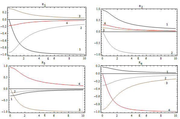
ψi​n,j=exp⁡(−ⅈ​k​r)​Rj​(k2),RS=(R1,R2,R3,R4),\psi_{in,j}=\exp(-\rmi kr)R_{j}(k^{2})\,,\qquad R_{S}=(R_{1},R_{2},R_{3},R_{4})\,, (92)

given by columns Rj​(k2)R_{j}(k^{2}) of matrix RSR_{S} which scatter just with a phase shift (86),

ψo​u​t,j=exp⁡(ⅈ​k​r+2​ⅈ​δ0​(k,aj))​Rj​(k2).\psi_{out,j}=\exp(\rmi kr+2\rmi\delta_{0}(k,a_{j}))R_{j}(k^{2})\,. (93)

Vectors R→j\vec{R}_{j} depends on the energy of ingoing wave. In Figure 3 we show this dependence for a particular example ℰ=4.5​ⅈ{\cal E}=4.5\rmi. Changing two complex parameters bb and E we can manipulate transitions between channels which may open a way for broad physical application of EPP SUSY transformations.
Refer to caption
Figure 3: Eigenvectors of the scattering matrix S2S_{2}.

4 Conclusion

In the present paper we have generalized two-channel eigen-phase preserving SUSY transformations to the multichannel case, N=2​M>2N=2M>2. It was surprising, that such generalization exists for even number of channels only. A single EPP SUSY transformation depends on a complex factorization energy ℰ{\cal E}, and M×MM\times M complex matrix BB, such that BT​B=INB^{T}B=I_{N}. Therefore single EPP SUSY transformation provide an M⁡(M−1)+2M(M-1)+2 parametric deformation of scattering matrix without affecting eigen-phase shifts.

There are several possible applications of presented results. One can use EPP SUSY transformations to solve inverse scattering problem by deforming a diagonal S-matrix as in [3]. We also may consider the S-matrix eigenvalues which conserved under M⁡(M−1)+2M(M-1)+2 parametric deformation as integrals of motions for some dynamical system associated with matrix Schrödinger equation [4]. In this context it is interesting to establish how this dynamical system looks. We expect that in this way new exactly solvable non-linear equations may be discovered.

Acknowledgements

AMP thanks Brazilian foundation CAPES (Coordenação de Aperfeiçoamento de Pessoal de Nìvel Superior) for the financial support. This work is supported by RFBR grant N. 12-02-31552.

References

References

  • [1] Taylor J R 1972 Scattering Theory: The Quantum Theory on Nonrelativistic Collisions (New York: Wiley)
  • [2] Sparenberg J-M, Pupasov A M, Samsonov B F and Baye D 2008 Exactly-solvable coupled-channel models from supersymmetric quantum mechanics Mod. Phys. Lett. B 22 2277-86
  • [3] Pupasov A, Samsonov B F, Sparenberg J M and Baye D 2011 Phys. Rev. Lett. 106 152301
  • [4] Matveev V and Salle M 1991 Darboux Transformations and Solitons (New York: Springer)
  • [5] Cannata F and Ioffe M V 1993 Coupled channel scattering and separation of coupled differential equations by generalized Darboux transformations J. Phys. A: Math. Gen 26 L89-92
  • [6] Samsonov B F, Sparenberg J-M and Baye D 2007 Supersymmetric transformations for coupled channels with threshold differences J. Phys. A: Math. Theor. 40 4225-40
  • [7] Pupasov A M, Samsonov B F and Sparenberg J-M 2008 Exactly-solvable coupled-channel potential models of atom-atom magnetic Feshbach resonances from supersymmetric quantum mechanics Phys. Rev. A 77 012724 (Preprint quant-ph/0709.0343)
  • [8] Levitan B M 1984 Inverse Sturm-Liouville Problems (Moscow: Nauka)
  • [9] Chadan K and Sabatier P C 1989 Inverse Problems in Quantum Scattering Theory, 2nd edn. (New York: Springer).
  • [10] Baye D and Sparenberg J-M 2004 Inverse scattering with supersymmetric quantum mechanics J. Phys. A: Math. Gen. 37 10223-49
  • [11] Pupasov A M, Samsonov B F, Sparenberg J M and Baye D 2010 J. Phys. A 43 155201
  • [12] Baye D 1987 Supersymmetry between deep and shallow nucleus-nucleus potentials Phys. Rev. Lett. 58 2738-41
  • [13] Sparenberg J-M and Baye D 1996 Supersymmetry between deep and shallow optical potentials for 16O + 16O scattering Phys. Rev. C 54 1309-21
  • [14] Sparenberg J-M and Baye D 1997 Supersymmetry between phase-equivalent coupled-channel potentials Phys. Rev. Lett. 79 3802-5
  • [15] Samsonov B F and Stancu F 2002 Phase equivalent chains of Darboux transformations in scattering theory Phys. Rev. D 66 034001
  • [16] Samsonov B F and Stancu F 2003 Phase shifts effective range expansion from supersymmetric quantum mechanics Phys. Rev. C 67 054005
  • [17] Amado R D, Cannata F and Dedonder J-P 1988 Coupled-channel supersymmetric quantum mechanics Phys. Rev. A 38 3797-800
  • [18] Amado R D, Cannata F and Dedonder J-P 1990 Supersymmetric quantum mechanics coupled channels scattering relations Int. J. Mod. Phys. A 5 3401-15
  • [19] Leeb H, Sofianos S A, Sparenberg J-M and Baye D 2000 Supersymmetric transformations in coupled-channel systems Phys. Rev. C 62 064003
  • [20] Amado R D, Cannata F and Dedonder J-P 1988 Formal scattering theory approach to S-matrix relations in supersymmetric quantum mechanics Phys. Rev. Lett. 61 2901-4