Relevance of coordinate and particle-number scaling in density functional theory
Abstract
We discuss a -dependent family of electronic density scalings of the form in the context of density functional theory. In particular, we consider the following special cases: the Thomas-Fermi scaling ( and ), which is crucial for the semiclassical theory of neutral atoms; the uniform-electron-gas scaling ( and ), that is important in the semiclassical theory of metallic clusters; the homogeneous density scaling () which can be related to the self-interaction problem in density functional theory when ; the fractional scaling ( and ), that is important for atom and molecule fragmentation; and the strong-correlation scaling ( and ) that is important to describe the strong correlation limit.
The results of our work provide evidence for the importance of this family of scalings in semiclassical and quantum theory of electronic systems, and indicate that these scaling properties must be considered as important constraints in the construction of new approximate density functionals. We also show, using the uniform-electron-gas scaling, that the curvature energy of metallic clusters is related to the second-order gradient expansion of kinetic and exchange-correlation energies.
pacs
71.10.Ca,31.15.E-,31.10.+zI Introduction
In Density Functional Theory (DFT) [1, 2, 3], the density scaling is a key concept and was used along the years to derive many exact constraints [4, 5, 6, 7, 8, 9, 10, 11, 12], as well as useful virial relations [13, 4, 14, 15, 16, 17, 18] for the kinetic, exchange and correlation energy functionals. Furthermore, the density scaling has a fundamental role in DFT due to its intimate relation with the adiabatic connection formalism [4, 19, 20].
One important family of scaling transformations for the particle density is defined by the general linear transformation [5]
| (1) |
where is a real invertible matrix and . Scaling transformations of this kind correspond to changing the external potential associated with the density whilst preserving the normalization of the density, i.e.
| (2) |
The most important scalings connected with Eq. (1) are the ones defined by
| (3) |
i.e., with a diagonal matrix with positive elements. In particular, there are three cases of high physical interest:
(i) the uniform scaling defined by , hence . Under uniform scaling the Kohn-Sham exchange and the non-interacting kinetic energies transform as and , respectively [4]. However, the interacting kinetic energy and the non-local Hartree-Fock exchange energy do not have these properties [4]. All popular exchange and kinetic energy functionals are nowadays designed to satisfy the uniform scaling relation [2, 3].
(ii) The two-dimensional nonuniform scaling of the density defined by and , hence , under which the system approaches the 1D limit when . Although there are important conditions for both Kohn-Sham exchange and correlation energies under this scaling [5], they are not satisfied by any popular XC functional (to our knowledge).
(iii) The one-dimensional nonuniform scaling of the density defined by and , hence , under which the system approaches the 2D limit when . This density scaling, that is related to the dimensional crossover of the XC energy (from 3D to 2D) [22, 23, 24], has been recently incorporated in a semilocal XC functional, named q2D-generalized-gradient-approximation (q2D-GGA) [25], constructed for mild and strong quasi-2D regimes. The remarkable performance of the q2D-GGA for surface energies and lattice constants of transition metals, showed the power of the one-dimensional nonuniform scaling.
In this paper we consider a different type of scaling for the density and focus the attention on the family of scaling relations of the form
| (4) |
where is a parameter. These scaling transformations differ from those defined by Eq. (1) in the fact that they do not only change the external potential associated with the density , but also provide a change in the particle number (). Well known members of the scaling family defined by Eq. (4) are the Thomas-Fermi [26, 27] and the homogeneous density scaling [9], which are relevant for the semiclassical theory of the many-electron, non-relativistic, neutral atom [26], and for the self-interaction error [9], respectively. (Unless otherwise stated, atomic units are used throughout, i.e., .)
This article is organized as follow: in Section II we shortly review the fractional-particle density functional theory, that is the correct framework for the scalings of Eq. (4); in Section III we present scalings properties of useful density functionals; Section IV is devoted to the physical properties of selected density scalings (for =1/3, -1/3, 0, 1, and -1); and in Section V we briefly analyze the performance of popular density functionals for the above scalings. Finally, in Section VI we summarize our conclusions.
II Theory and definitions
Under the scaling transformations defined by Eq. (4) the normalization of the particle density is modified, thus the number of particles in the system is varied as , with being in general a non-integer number. The conventional picture of DFT, based on the Hohemberg-Kohn theorems [28] and/or the Levy constrained search [29] is thus inappropriate in this case. In fact, a proper definition of densities with a non-integer number of particles is required in this case [30, 31, 32]. In this work we achieve this through the introduction of ensembles densities within a zero-temperature grand canonical ensemble theory [30].
The central quantity to consider is therefore the density-matrix operator [3]
| (5) |
where the sums are extended over all possible particle numbers and over all the states of the -particle Hamiltonian, is the -th eigenstate of the -particle Hamiltonian and is the probability weight to find the system in the eigenstate (hence, we have and ). The expectation value of any operator is consequently obtained as . In particular, for the particle density we have
| (6) |
where we defined the super-index , is the pure-state density of the -particle -th state, and we used
| (7) |
with and the single-particle orbital and annihilation operator of state , respectively. The total number of particles is, according to Eq. (6),
| (8) |
Similarly, for the one-particle density-matrix operator we have and
| (9) |
The ensemble Hohemberg-Kohn universal functional and the non-interacting kinetic energy are defined as [3]
| (10) | |||||
| (11) |
where is the electron-electron repulsion operator and the kinetic energy operator is defined by
| (12) |
The electron-electron repulsion operator can be further decomposed into Coulomb, exchange, and correlation contributions to yield
| (13) | |||||
| (14) | |||||
| (15) |
where is the density-matrix operator minimizing either or , according to Eqs. (10) and (11), and with the exchange energy operator defined as [3]
| (16) |
while no explicit expression is known for . Note that all the traces can be easily evaluated by use of Eqs. (6) and (9), together with the resolution of identity .
Within the theoretical framework sketched above the scaling relations of Eq. (4) can be interpreted as an uniform scaling of the pure-state densities ( ) accompanied by a remodulation of the statistical weights such that the particle number is changed to . Note that this latter is in general a complicated transformation because it must accomplish the required particle-number variation preserving the correct density and without violating the normalization conditions for the statistical weights ( and ). In particular, the simple transformation in general is not a suitable transformation, as it brings a violation of the normalization conditions. Nevertheless, one special case is when we consider a system with one electron or less and . In this case in fact the density of fractional charge can be written , where and are the densities for one particle and zero particles, respectively (the latter is of course identically zero everywhere). The scaling transformation yields then . Thus, in this special case we have indeed (all information concerning the term can be neglected). This important result will be employed in next section to derive exact scaling relations for the non-interacting kinetic energy and the Kohn-Sham exchange for systems with fractional occupation.
More insight into the properties of the transformation governing the statistical weights can be achieved by considering (in analogy with the usual adiabatic connection procedure) the M-particle Hamiltonian with a local potential which gives the right pure-state densities to recover Eq. (4). In this way the trasformation of the statistical weights, connected to scaling transformations of the type defined in Eq. (4), can be defined explicitly in two separate cases. When, upon scaling, the variation in the particle number is smaller than one (i.e., or similarly ), the statistical weights change with as
| (17) |
and consequently, the exact total energy functional varies linearly with [30]
| (18) |
where and denote - and -densities. When the variation in the particle number is larger than one (i.e., the number of particles changes from to , with an integer and ), the statistical weights change as
| (19) |
Therefore, the transformation can be seen as a chain of transformations like the one in Eq. (17) concerning successively , , , , . As a consequence, the exact total energy functional will be described as a succession of straight lines. Thus, the derivative discontinuity [30] plays an important role for the scaling transformations, especially when and are finite. However, in the limit the role of derivative discontinuity is diminished and one can always consider . In this case the behavior of the system is closely related to the semiclassical physics, as shown in the next sections. Because of the complexity of this density scaling, in this paper we mainly consider only two extreme cases of interest: when and , and the semiclassical limit .
III General scaling properties
Using the definition of Eq. (4) we can immediately find the scaling properties of several quantities which depend explicitly on the particle density. This is the case, for example, of the the Coulomb energy and any external potential (e.g., with ). Hence,
| (20) | |||||
| (21) |
Another interesting quantity is the local Seitz parameter which scales as
| (22) |
Therefore, for we have that implies , while implies . Thus, the conditions and correspond to scalings to the high- and low-density limits, respectively. The opposite is true for . For the special case instead the local Seitz parameter is independent on and the density regime cannot be modified by a scaling transformation.
On the other hand, the usual density parameters , , , and , with being the local Fermi wave-vector [33, 34], being the Thomas-Fermi screening wave-vector [33, 34], and being the wave vector suitable for bonding and valence regions [35], scale according to
| , | (23) | ||||
| , | (24) |
Thus, the reduced gradient and Laplacian for exchange and kinetic energies ( and ) are independent on so that the slowly-varying density limit () is reached whenever , while for a rapidly-varying density regime is always set up. On the contrary the density parameters and , which are relevant for the correlation, have a dependence on . Therefore, they can describe different density regimes depending on the actual value of the parameter .
Because for any value of the reduced gradient for exchange and kinetic energy and the reduced Laplacian become small in the limit , it is also interesting to investigate the scaling behavior of local density approximations (LDA) and gradient expansions for the non-interacting kinetic energy and the exchange energy. These expressions will in fact become almost exact in the limit . The required scaling relations are given by the formulas
| (25) | |||||
| (26) | |||||
| (27) | |||||
| (28) | |||||
| (29) |
where is the second-order gradient correction (GE2) term of the exchange energy [36], is the second-order gradient correction term of the non-interacting kinetic energy [2], is the von Weizsäcker kinetic energy functional [2], and is the fourth-order kinetic energy gradient expansion term (GE4) [37, 38]. Using these expressions, as well as Eq. (20), it is possible to provide an useful accurate approximation for the universal functional of Eq. (10) in the slowly-varying limit ():
| (30) | |||||
In this formula we neglected correlation contributions. In fact, the leading term of LDA correlation energy in the high-density limit is [39] , and does not respect any simple scaling; whereas the leading term in the low density limit is [39] , and scales as . Moreover, the second-order correction to the correlation energy [40] scales always as . However, due to the dependence on of the reduced gradients and , the slowly-varying limit is only reached for . In addition, for any the scaling to the slowly-varying limit corresponds also to a scaling to the high-density limit ( when ). In this limit the correlation contributions are negligible with respect to the exchange part, and thus Eq. (30) becomes almost exact. For however correlation corrections to Eq. (30) might be needed.
To conclude this section we consider briefly the cases of Kohn-Sham kinetic and exchange energies. Using the convexity arguments derived in Ref. [9], and taking into account that the scaling family of Eq. (4) can be seen as an uniform scaling followed by a homogeneous scaling (i.e. ), the following inequalities hold:
| (31) | |||
| (32) |
and
| (33) | |||
| (34) |
Moreover, using the rigorous bound , and the one conjectured by Lieb [27] (for a rigorous, and tighter upper bound of in terms of , and , see Eq. (23) of Ref. [41]), we can easily derive the following inequalities
| (35) |
for any and . In the case of exchange energy, the Lieb-Oxford bound [42, 43, 44] gives
| (36) |
In the special case of one particle or less () and , using the formalism presented in Section II (especially the fact that ) it can be shown (see Appendix A) that
| (37) |
and
| (38) |
These results correctly agree with the scalings of and , because in case , and [45]. (Note also that Eq. (37) holds for [45].)
IV Selected scaling relations
In this section we analyze in more detail the scaling relations corresponding to special values of the parameter . In this way we can highlight the physical significance of the family of scaling transformations defined by Eq. (4) and provide evidence for its importance in electronic structure theory.
IV.1 Thomas-Fermi scaling ()
If we require the LDA non-interacting kinetic energy to scale as the Coulomb energy, we find , which corresponds to the well known Thomas-Fermi scaling [26]. With this choice the scaling of the density and the reduced gradients are
| , | (39) | ||||
| , | (40) | ||||
| , | (41) |
Thus, for the high-density limit is reached and the exchange and kinetic energies, whose behavior is controlled by the density parameters and , are in a slowly-varying density regime. Therefore, the universal functional can be written [26]
| (42) | |||||
and the Thomas-Fermi kinetic energy () and the classical Coulomb energy are the leading terms in the total electronic energy ( scales as ). This result is very important. In fact, the semiclassical theory of the many-electron neutral atom [46, 47, 48] is based on Eq. (42), which leads to the semiclassical asymptotic expansion for the kinetic energy
| (43) |
and a similar one for exchange [49], that are very accurate (typical error of order 0.5% - 0.2% even for real atoms [26, 49, 50]). Note that the second term in the kinetic energy expansion (), can not be captured by the Thomas-Fermi scaling, being a quantum correction. Recently, it has been demonstrated that these asymptotic expansions are also important tools in DFT [26, 51, 52, 53], as they have been used to construct accurate non-empirical exchange-correlation [51] and kinetic [52] energy functionals.
Extensions of Eq. (43) have been also proposed for general ions and atoms [54, 55, 56, 57], which constitute a more challenging problem than neutral atoms alone. However, even for the first ionization potential of many-electron atoms, the extented semiclassical Thomas-Fermi theory shows serious drawbacks and limitations [58], and accurate results can be obtained only within Kohn-Sham DFT or other orbital-dependent schemes.
Concerning correlation, we can obtain some insight by considering that, any reasonable generalized gradient correction to the LDA correlation must be designed to cancel the logarithmic divergence of the LDA term under uniform scaling to the high density limit [59]. Thus, in the high-density limit . However, under the Thomas-Fermi scaling , while , so that correctly for ( is a density parameter suitable for valence and tail regions that are evanescent in a many-electron neutral atom), the density parameter is just independent on . Hence, the gradient corrections to the correlation are independent on the scaling and the whole correlation energy is dominated by the LDA contribution for . As a consequence, popular GGA functionals (e.g. PBE [59]) that recover LDA correlation in this limit, can be argued to be accurate (exact) [26].
Finally, we mention the importance of the Thomas-Fermi scaling also for the atomic densities. In fact, under a Thomas-Fermi scaling to the high-density limit, the hydrogenic density resembles features of the Thomas-Fermi density [60], becoming slowly-varying over a Fermi wavelength (but not over the screening length ). We recall that the Thomas-Fermi density, even if does not show shell structure and does not decay correctly, is a very good model for the densities of heavy atoms [61, 62, 63, 50]. For an excellent discussion, see Ref. 26.
IV.2 Uniform-electron-gas scaling ()
Consider a generic density parameter . We define the uniform-electron-gas (UEG) scaling, as the scaling belonging to the family of Eq. (4) that makes small for any value of in the limit . It is easy to prove that this scaling is defined by the parameter . Under such a scaling the density and the reduced gradients behave as
| , | (44) | ||||
| , | (45) | ||||
| , | (46) |
Thus, both the density and the local Seitz parameter are independent on (except for a coordinate scaling), so that the scaling does not involve any transformation towards the high- or low-density limit. On the contrary, by construction, all the density parameters vanish in the limit , so the slowly-varying density limit is fully recovered in this case (hence, the name uniform-electron-gas scaling). Interestingly, Eqs. (45) and (46) also show that for first-order density parameters (i.e. those depending on ) exactly the same dependence on is found under the uniform-electron-gas scaling.
For large values of the universal functional is well approximated by
| (47) | |||||
where the full LDA correlation energy is considered in Eq. (47). Of course, in the limit the LDA approximation of becomes exact (all the density parameters vanish in this limit, by construction). In particular, we have
| (48) |
where . Note that while this constraint is satisfied by most non-empirical XC semilocal functionals (that recover the LDA for a constant density), it can be out of reach for some wavefunction methods, as the second-order perturbation theory of Møller-Plesset (MP2) and its modifications [64, 65], or the random phase approximation (RPA) [66, 67]. However, the sophisticated orbital-based inhomogeneous Singwi-Tosi-Land-Sjölander (ISTLS) method [68, 69], as well the XC kernel of linear response time-dependent DFT (in the context of the adiabatic-connection fluctuation-dissipation theorem [70, 71, 66]) of Ref. [72], are accurate for the uniform-electron-gas scaling.
To provide an example of the utility of the uniform-electron-gas scaling let us consider neutral jellium clusters with electrons and radius , having the external potential
| (49) |
due to a positive background density
| (50) |
This external potential has no singularities, so the reduced gradients and Laplacian of the density, are finite everywhere inside the bulk. Moreover, the values of the density parameters decrease for increasing number of electrons . Indeed, even for intermediate values of , the density is slowly varying over a Fermi wavelength, so the extensions of Thomas-Fermi theory become accurate [73, 74, 75, 83].
Jellium clusters with different numbers of electrons may be thought therefore to be well described by the uniform-electron-gas scaling, since under the scaling procedure the number of electrons is changed to , the local Seitz parameter is kept fixed to , and the reduced gradients are decreased as , in full analogy to what happens in the jellium clusters. The relation between the uniform-electron-gas scaling and the jellium clusters can be in fact clearly recognized by a detailed analysis of the cluster’s electron densities.

To this end, in Fig. 1 we show the densities of and Na jellium clusters, together with the UEG-scaled density of the cluster where a value was used. Remarkably, the scaled density agrees very well with the cluster density showing that the variations of the physical properties of the different clusters with can be well captured by the uniform-electron-gas scaling. Note that the small differences between the scaled and the true density are due to quantum oscillations [83] that are not accounted by the scaling procedure, but are of course included in the self-consistent Kohn-Sham scheme. These are however not very relevant for the analysis that we consider henceforth.
The total energy of a jellium cluster can be written
| (51) |
Therefore, using the uniform-electron-gas scaling for we can write
| (52) | |||||
where we used the fact the Coulomb and external potentials cancel each other in the limit of a large number of electrons. This expression agrees well with the asymptotic expansion of the total energy of the clusters derived from the liquid drop model [73, 74, 75] (recall that )
| (53) |
where is the volume (bulk) energy and and are the surface and curvature energies. A comparison of the first terms (those scaling as ) in Eqs. (52) and (53) shows in fact that the uniform-electron-gas scaling correctly yields . Moreover, similar with the previous Thomas-Fermi scaling (see Eq. (43)), the second term in Eq. (53) is a quantum oscillation term, that apparently can not be described by the simple UEG scaling, without a careful analysis of the Friedel oscillations near the surface of the cluster. Finally, the third term is related to the curvature energy
| (54) |
This is an important result, because the real edge gas contains curvature corrections [76], that until now had not been addressed.
IV.3 Homogeneous density scaling ()
The homogeneous density scaling [9, 11, 77, 78, 79, 80, 81, 82] is obtained from Eq. (4) by setting the parameter . Under this condition the scaling relations for the density and the various density parameters are
| , | (55) | ||||
| , | (56) | ||||
| , | (57) |
For the high-density slowly-varying limit is obtained and the universal functional is well approximated as
| (58) | |||||
In this case the functional of Eq. (58) is dominated by the classical Coulomb term, and the second leading term is the Thomas-Fermi kinetic energy. (Note that the nuclear energy grows only linearly with .)
More importantly, the homogeneous scaling is a valuable tool to investigate DFT, when the opposite limit, i.e. with , is considered. For this case in fact several studies exist on the scaling properties and exact constraints of the kinetic and exchange energy functionals [9, 11] as well as on the static correlation treatment in DFT [84, 85]. In this work we focus instead on the role of the homogeneous scaling in the determination of the delocalization error [85] of the exchange(-correlation) functionals. To this end we consider the simple H dissociation problem, that is associated with the hydrogen atom with fractional charge [84], and compute
| (59) |
where for the hydrogen atom and is the partial electronic charge. The quantity represents thus the Coulomb and XC energy difference between the dissociation of H into one hydrogen atom plus one proton and that of the dissociation into two hydrogen atoms with fractional electron charge and . For the exact exchange-(correlation) functional it shall be zero at any value of . However, due to the one-electron self-interaction error [8], for approximated XC functionals for any , indicating that a fractional dissociation is favorable with respect to the exact one.
| X-only functionals | XC functionals | |||||
|---|---|---|---|---|---|---|
| Functional | Ref. | SIE | Functional | Ref. | SIE | |
| LDAx | [86, 87] | 44.5 | LDA | [86, 87, 92] | 22.3 | |
| PBEx | [59] | 6.6 | PBE | [59] | 5.8 | |
| APBEx | [51] | 1.8 | APBE | [51] | -3.4 | |
| revPBEx | [88] | 2.0 | revPBE | [88] | -4.0 | |
| PBEsolx | [89] | 19.8 | PBEsol | [89] | 11.9 | |
| zPBEsol | [89, 93] | 0.0 | ||||
| PBEintx | [90] | 16.9 | PBEint | [90] | 9.7 | |
| zPBEint | [90, 93] | 0.1 | ||||
| B88 | [91] | 2.7 | ||||
For a generic exchange functional we can assume (see Section V) the scaling , with . Thus, Eq. (59) becomes
| (60) | |||||
with the density of the hydrogen atom and Ha. Note that in this case correlation plays no role, since for the correlation energy is zero. Nevertheless for semilocal functionals, which are not self-correlation free, it is also possible to consider an in place of . Now, in analogy with Ref. 8, we can define the self-interaction error as
| (61) |
Equation (60) then becomes
| (62) |
with . A plot of for several values of is provided in Fig. 2.

Equation (62) shows that is always positive whenever the self-interaction error is not zero and the scaling behavior of the functional differs from the exact one (), since and is in general positive. Moreover, due to the form of the function , a symmetric fractional dissociation is always favored. The most important result of Eq. (62) is however the fact that the delocalization error (or dissociation error in H) has a twofold origin and only the second term on the right hand side depends on the self-interaction error for the hydrogen atom. The remaining contribution traces back only to the wrong behavior of the functional under the homogeneous scaling. Note also that the first term might be the dominant one since the SIE is typically one order of magnitude smaller than the Coulomb energy in the H atom (see Table 1 for the value of for some popular functionals).
This result shows the importance of the homogeneous density scaling in the development of accurate XC functionals. In fact, several functionals were constructed to minimize the self-interaction error of the hydrogen atom [94], but no semilocal approximation exists that provides the correct scaling behavior under uniform density scaling.
IV.4 Fractional scaling ()
Let consider the disintegration of the hydrogen atom into two neutral atoms having a fractional number of electrons and corresponding fractional nuclear charge. The electron density of the hydrogen atom with a fractional number of electrons , must be considered as the ensemble density given by the superposition of the density of an hydrogen atom with one electron and nuclear charge , with weight , and that of one hydrogen atom with no electrons and nuclear charge , with weight zero (this latter thus does not contribute). Recalling that for the hydrogen atom, a scaling of the nuclear charge corresponds to an uniform scaling of the density, we find that
| (63) |
Generalizing the result of Eq. (63), we define the fractional scaling as the scaling obtained from the family of relations given in Eq. (4) when . Under this scaling the density and the various density parameters behave as
| , | (64) | ||||
| , | (65) | ||||
| , | (66) |
In the limit the system is scaled towards the high-density limit () and the universal functional is well approximated as
| (67) | |||||
Note however that in this limit the reduced gradients for the correlation are not small (and thus the correlation energy is not important). Eq. (67) shows a particular classical behavior of the electrons: their kinetic energies become dominant over the classical Coulomb and exchange energies. Thus, in the limit , the electronic system shows similarities with a gas of non-interacting particles, with non-uniform density .
In the opposite limit (), the fractional scaling describes, as discussed above, the scaling towards a fractional atom. In fact, in this case the system is correctly scaled towards the low-density limit with the reduced gradient and Laplacian for the kinetic and exchange energy becoming large. To strengthen the significance of such a scaling we consider its application to the disintegration of an atom, as introduced above. For simplicity we consider the disintegration of a hydrogen atom into two neutral atoms having a fractional number of electrons and , respectively, and corresponding fractional nuclear charge. We define the XC disintegration energy as
| (68) |
where denotes the XC energy of the H atom with fractional electron number and nuclear charge . Note that correlation will only play a role when approximate non-self-interaction-free DFT functionals are considered (), while only exchange will contribute in the computation of . This quantity is very important since the accuracy of any GGA functional in computing the values of is directly related to its ability to predict good atomization energies, because both processes (disintegration and atomization) preserve the total number of electrons. This fact is clearly shown in Fig. 3 where it can be noted the linear relation between the mean absolute error (MAE) on the computation of atomization energies of organic molecules (we considered here the AE6 test [95], which is representative for organic molecule atomization energies) and the disintegration error defined as
| (69) |
for several representative XC functionals. Of course, a linear relation is obtained as well with the errors on the XC energy of a Gaussian one-electron density, which was shown to be a model system for atomization energies [35, 93].
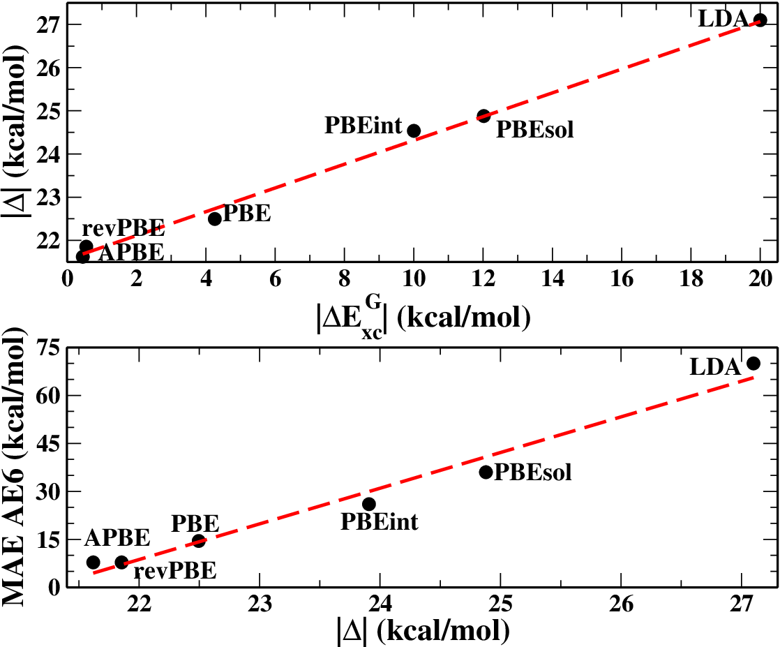
The disintegration error can be written alternatively
| (70) |
For the exact energy we have , while for the approximate functionals we found numerically (see section V) with 2.3. Substituting into Eq. (70) we obtain
| (71) |
Equation (71) shows that: (i) the hydrogen disintegration problem is not related to the hydrogen one-electron density, as might appear at a first sight. Indeed, for a GGA which is exact for the hydrogen atom we would have 22 kcal/mol. In fact, Fig. 3 shows that the hydrogen atom disintegration is rather linearly related to the Gaussian one-electron density. (ii) The error is determined basically from the behavior of the functional for =1. (iii) To minimize the disintegration error (and thus yield good atomization energies), must be about 10-20% larger than for the hydrogen atom; this condition is well met by GGA functionals accurate for atomization energies (APBE [51], revPBE [88]), and is also well satisfied by the recently proposed zvPBEsol, and zvPBEint [35]. However, this result shows that in fact all these functionals base their performace on an error cancellation effect which is made inevitable by their inability to respect the fractional scaling.
Thus, the fractional scaling appears as an important exact constraint that XC functionals should respect. At present all popular approximations to the XC energy are only designed to respect the uniform scaling and are unable to fulfill the fractional scaling relations.
IV.5 Strong-correlation scaling ()
For , and in the semiclassical limit , starts to dominate over the Thomas-Fermi kinetic energy , and thus the system may reach a strongly-correlated limit. Let us briefly consider the case .
With this choice the scaling of the density and the reduced gradients are
| , | (72) | ||||
| , | (73) | ||||
| , | (74) |
and thus, under this scaling with , the system is in a slowly-varying, low-density limit. Thus, our approximation for the universal functional becomes
| (75) | |||||
which shows that the kinetic energy of the electrons, is much smaller than the Coulomb interaction, and the system resembles the features of a Wigner crystal, being in a strongly-correlated limit. Note that in this limit, the LDA correlation energy scales as , being as important as the exchange part. We recall that such a Wigner crystal is well described by a semilocal functional (see Eq. (23) of Ref. [101]) derived from the point-charge-and-continuum (PC) model [101]. Note that the PC model was incorporated in high-level methods (e.g. ISI method of Ref. [102]), and recent excellent work has been done for further development of the PC model, see Refs. [103, 104], as well for a DFT of strongly-correlated systems [105, 106]. Thus, further study of this scaling can be important.
| Functional | Ref. | ||
|---|---|---|---|
| Exchange-only functionals | |||
| LDAx | [86, 87] | 1.333 | 2.666 |
| B88 | [91] | 1.254 | 2.206 |
| PBEx | [59] | 1.266 | 2.323 |
| APBEx | [51] | 1.262 | 2.316 |
| revPBEx | [88] | 1.252 | 2.252 |
| PBEsolx | [89] | 1.280 | 2.356 |
| PBEintx | [90] | 1.272 | 2.329 |
| TPSSx | [99] | 1.297 | 2.399 |
| revTPSSx | [100] | 1.309 | 2.439 |
| Exact | 2.000 | 3.000 | |
| Exchange-correlation functionals | |||
| LDA | [86, 87, 92] | 1.317 | 2.517 |
| PBE | [59] | 1.272 | 2.342 |
| APBE | [51] | 1.268 | 2.333 |
| revPBE | [88] | 1.258 | 2.271 |
| PBEsol | [89] | 1.287 | 2.378 |
| zPBEsol | [89, 93] | 1.268 | 2.316 |
| PBEint | [90] | 1.279 | 2.351 |
| zPBEint | [90, 93] | 1.261 | 2.289 |
| Exact | 2.000 | 3.000 | |
V Effective scaling for semilocal functionals
In this section we consider an assessment of semilocal XC density functionals for various scalings discussed above. In previous sections we discussed the scaling properties of several exact energy functionals under the scaling transformations of the type of Eq. (4) and we proved the utility of such scaling relations in various contexts. At the same time, we noted that these scaling relations are not respected by approximate functionals even at the LDA or second-order gradient-corrected level (the von Weizsäcker kinetic energy functional being one exception). The situation is even worst for generalized gradient approximations which indeed do not have a well defined scaling behavior under the scaling transformations of Eq. (4).
Nevertheless, it can be seen that most XC functionals in fact display an effective scaling . Solving this equation for the parameter , we find . Therefore, it is conceivable to define an effective scaling order for a generic functional as
| (76) |
Because our interest for the scaling of general exchange(-correlation) functionals in this work was motivated by the homogeneous and fractional scaling, we restricted our definition to use of hydrogen density and the interval , where we can compare with exact results.
The effective scaling order provides a measure for the scaling behavior of different functionals, resembling in this respect the effective homogeneity of XC functionals [96, 97, 98]. Of course, for functionals having a well defined scaling behavior (e.g. LDAx), the effective scaling order will coincide with the analytic scaling exponent. For other functionals it will provide a measure of the effective scaling behavior, so that the deviations of the effective scaling order from the true value could give an estimation of the accuracy of the functional to fulfill the scaling relation. We note that for the latter cases the integrand of Eq. (76) was always found to be almost constant over the entire integration interval (except very close to the boundaries; note however that the function is integrable over the given range), showing the robustness of our definition.
In Table 2 we report the values of for several exchange and exchange-correlation functionals at and . An inspection of the data shows that all the functionals perform similarly and quite differently from the exact reference, that in this case is the exact Kohn-Sham exchange, since for and there is no correlation. Remarkably, the best scaling behavior is found for LDA exchange, while slightly worst results are obtained for GGA functionals. The use of meta-GGA functionals, as TPSS [99] or revTPSS [100], which are constructed taking into account the physics of one-electron systems, is found finally to bring a slight improvement in the effective scaling behavior. Moreover, at the GGA level the addition of approximate correlation seems to bring some small improvement in the scaling behavior, in line with the fact that indeed semilocal DFT functionals are not really exchange or correlation functionals but rather rely on an heavy error compensation between the two. We recall instead that meta-GGA functionals are one-electron-self-correlation free.
VI Conclusions
In summary, we have investigated the scaling with variable particle number of the form of Eq. (4): . For such scaling transformations we provided a formal definition within the ensemble formalism of DFT and studied the basic features, also in relation to the scaling properties of different important density functionals.
The density scalings defined in Eq. (4), spans an impressive set of physical properties: in the limit of large they are crucial for semiclassical theory of many-electron systems (e.g. Thomas-Fermi scalings is related to atoms, Uniform-electron-gas scaling is related to metallic clusters, strong-correlation scaling is related to Wigner crystals), whereas in the limit of small they are connected with the physics of small systems with fractional particle number, and to self-interaction errors.
The here proposed uniform-electron-gas scaling () is the right basic concept for jellium clusters. Simple scaling manipulations showed that the curvature corrections are in fact related to the second-order gradient expansion. On the other hand, the surface corrections (described by the Airy gas model [76]), are quantum oscillations terms. By analogy with the recent work on the semiclassical atom [26, 50, 49], a modified second-order gradient expansion (MGE2) can be constructed for jellium clusters, in order to recover the exact surface corrections. However, we expect that such a MGE2 will be very close to the regular GE2 that is accurate for surfaces of simple metals when the Kohn-Sham densities are used [89].
Moreover, the idea of MGE2, that can account for the principal quantum corrections, can be generalized for any (in the limit of large ). Such a MGE2 will be very useful especially for the strongly-correlated scaling () where the LDA term is not exact (in the limit ) due to the self-interaction problem in Wigner crystals [101]. For example, MGE2 for the exchange energy may have the form
| (77) |
where and should be derived in further investigations. (For the Thomas-Fermi scaling and [49]; whereas the regular GE2 has and ).
Finally we have shown the usefulness of the here proposed fractional scaling () for the atomization energies of molecules. Recently, it has been derived an atomization energy constraint (i.e. minimization of an entropy-like function for an ensemble one-electron density models) [93, 35]. This constraint was derived from an empirical observation relating errors in the model one-electron densities to errors in the atomization energies, of popular GGAs (see Fig. 2 of Ref. [93]); and from the physical explanation that one-electron densities are simple models for simple bonding regions, where iso-orbital regime can be significant. (see Fig. 1 of Ref. [93], and the corresponding discussion). Using the fractional scaling (), we have better explained the significance of one-electron Gaussian model for atomization energy of molecules and disintegration of the hydrogen atom (see Eq. (71) and its related discussion).
We recall that the semilocal exchange hole models satisfy the sum rule for systems with integer number of electrons [108], but violate the exchange hole sum rule in case of fractional number of electrons, and thus predicting too-negative energies for such systems [109]. The here proposed effective scaling (see Section V), measures in fact the functional accuracy for systems with fractional particle number, and can be used to develop (and test) new better approximations.
Our work provides a deeper insight into the relevance of the scaling relations having the form defined in Eq. (4) and highlights the importance of these scaling relations in DFT. In particular, Eqs. (31)-(34) provide useful scaling relations with varying particle number that are important constraints in the construction of approximate exchange-correlation (or noninteracting kinetic) functionals. Moreover, for the limit, Eqs. (37) and (38) are exact constraints for the Kohn-Sham exchange and kinetic energy functionals, respectively and the effective scaling order (Eq. (76)) is a more general requirement, which is relevant for the SIE problem. Unfortunately, no such explicit expressions exist instead for the limit, where however the recovery of the semiclassical atom physics was shown to be an important condition.
Acknowledgments: We thank F. Della Sala for useful discussions and acknowledge funding by the European Research Council (ERC) Starting Grant FP7 Project DEDOM, grant agreement no. 207441.
Appendix A Scaling relations for Kohn-Sham kinetic and exchange energies for one electron systems
In this appendix we consider briefly the special case of a fractional number of particles (with ) and . In this case, using the formalism of Section II we can derive, in line with Ref. 4, the general scaling properties for the non-interacting kinetic energy and the Kohn-Sham exchange functionals. Under coordinate scaling the density operator is transformed into another valid density operator and because of the simple scaling behavior of the statistical weight we have . At this point we can write , where we used the fact that , and we note that, for any , if is a minimum so must be . Hence,
| (78) |
In a similar way it can be proved that
| (79) |
References
- [1] W. Kohn and L. J. Sham, Phys. Rev. , A1133 (1965).
- [2] R. M. Dreizler and E. K. U. Gross, Density Functional Theory, Springer (1990).
- [3] R. G. Parr and W. Yang, Density-Functional Theory of Atoms and Molecules, Oxford University Press, USA, 1994.
- [4] M. Levy and J. P. Perdew, Phys. Rev. A , 2010 (1985).
- [5] A. Görling and M. Levy, Phys. Rev. A , 1509 (1992).
- [6] Q. Zhao, M. Levy, and R. G. Parr, Phys. Rev. A 47, 918 (1993).
- [7] S. Ivanov and M. Levy, J. Phys. Chem. A 102, 3151 (1998).
- [8] Y. Zhang and W. Yang, J. Chem. Phys. 109, 2604 (1998).
- [9] G. K.-L. Chan and N. C. Handy, Phys. Rev. A 59, 2670 (1999).
- [10] J. Toulouse, P. Gori-Giorgi, and A. Savin, Int. J. Quant. Chem. 106, 2026 (2005).
- [11] A. Nagy, J. Chem. Phys. 123, 044105 (2005).
- [12] A. Nagy, Phys. Rev. A 84, 032506 (2011).
- [13] S. K. Ghosh and R. G. Parr, J. Chem. Phys. 82, 3307 (1985).
- [14] R. van Leeuwen and E. J. Baerends, Phys. Rev. A 51, 170 (1995).
- [15] F. G. Cruz, K. C. Lam, and K. Burke, J. Phys. Chem. A. 102, 4911 (1998).
- [16] M. Levy and P. W. Ayers, Phys. Rev. A 79, 064504 (2009).
- [17] A. P. Gaiduk , S. K. Chulkov, and V. N. Staroverov, J. Chem. Theory Comput. 5, 699 (2009).
- [18] P. D. Elkind and V. N. Staroverov, J. Chem. Phys. 136, 124115 (2012).
- [19] M. Levy, Phys. Rev. A 43, 4637 (1991).
- [20] Y. A. Wang, Phys. Rev. A 56, 1646 (1997).
- [21] M. Levy and H. Ou-Yang, Phys. Rev. A , 651 (1990); H. Ou-Yang and M. Levy, Phys. Rev. A , 155 (1990).
- [22] L. Pollack and J. P. Perdew, J. Phys.:Condens. Matter , 1239 (2000).
- [23] L. A. Constantin, J. P. Perdew, and J. M. Pitarke, Phys. Rev. Lett. , 016406 (2008); Phys. Rev. Lett. , 269902(E) (2008).
- [24] L. A. Constantin, Phys. Rev. B , 155106 (2008).
- [25] L. Chiodo, L. A. Constantin, E. Fabiano, and F. Della Sala, Phys. Rev. Lett. , 126402 (2012).
- [26] P. Elliott, D. Lee, A. Cangi, and K. Burke, Phys. Rev. Lett. , 256406 (2008).
- [27] E.H. Lieb, Rev. Mod. Phys. , 603 (1981).
- [28] P. Hohemberg and W. Kohn, Phys. Rev. 136, B864 (1964).
- [29] M. Levy, Proc. Natl. Acad. Sci. USA 76, 6061 (1979).
- [30] J. P. Perdew, R. G. Parr, M. Levy, and J. L. Balduz Jr., Phys. Rev. Lett. , 1691 (1982).
- [31] W. Yang, Y. K. Zhang, and P. W. Ayers, Phys. Rev. Lett. 84, 5172 (2000).
- [32] P. W. Ayers, J. Math. Chem. 43, 285 (2008).
- [33] D. C. Langreth and M. J. Mehl, Phys. Rev. Lett. , 446 (1981).
- [34] J. P. Perdew, K. Burke and Y. Wang, Phys. Rev. B , 16533 (1996).
- [35] L. A. Constantin, E. Fabiano, and F. Della Sala, J. Chem. Phys. , 194105 (2012) .
- [36] P. R. Antoniewicz and L. Kleinman, Phys. Rev. B , 6779 (1985).
- [37] C. H. Hodges, Can. J. Phys. , 1428 (1973).
- [38] M. Brack, B. K. Jennings and Y. H. Chu, Phys. Lett. , 1 (1976).
- [39] J. P. Perdew and Y. Wang, Phys. Rev. B , 13244 (1992).
- [40] C. D. Hu and D. C. Langreth, Phys. Rev. B , 943 (1986).
- [41] F.J. Gálvez and I. Porras, Phys. Rev. A , 3336 (1992).
- [42] E.H. Lieb and S. Oxford, Int. J. Quantum Chem. , 427 (1981).
- [43] M.M. Odashima and K. Capelle, J. Chem. Phys. , 054106 (2007).
- [44] R. Haunschild, M.M. Odashima, G.E. Scuseria, J.P. Perdew, and K. Capelle, J. Chem. Phys. , 184102 (2012).
- [45] E. Sagvolden and J. P. Perdew, Phys. Rev. A , 012517 (2008).
- [46] J. Schwinger, Phys. Rev. A , 1827 (1980); ,ibid. , 2353 (1981).
- [47] B.-G. Englert and J. Schwinger, Phys. Rev. A , 2339 (1984); ibid. , 26 (1985).
- [48] B.-G. Englert, Semiclassical Theory of Atoms, (Lecture Notes in Physics, Springer-Verlag, Berlin, 1988).
- [49] P. Elliott and K. Burke, Can. J. Chem. , 1485 (2009).
- [50] D. Lee, L. A. Constantin, J. P. Perdew, and K. Burke, J. Chem. Phys. , 034107 (2009).
- [51] L. A. Constantin, E. Fabiano, S. Laricchia, and F. Della Sala, Phys. Rev. Lett. , 186406 (2011).
- [52] S. Laricchia, E. Fabiano, L. A. Constantin, and F. Della Sala, J. Chem. Theory Comput. 7, 2439 (2011).
- [53] E. Fabiano, L. A. Constantin, and F. Della Sala, J. Chem. Theory Comput. 7, 3548 (2011).
- [54] N. H. March and R. J. White, J. Phys. B 5, 466 (1972).
- [55] N. H. March and R. G. Parr, Proc. Nat. Acc. Sci. USA 77, 6285 (1980).
- [56] Y. Tal and L. J. Bartolotti, J. Chem. Phys. 76, 4056 (1982).
- [57] P. W. Ayers, J. B. Lucks, and R. G. Parr, Acta Chim. Phys. Debricina 34-35, 223 (2002).
- [58] L. A. Constantin, J.C. Snyder, J.P. Perdew, and K. Burke, J. Chem. Phys. , 241103 (2010).
- [59] J. P. Perdew, K. Burke, and M. Ernzerhof, Phys. Rev. Lett. , 3865 (1996).
- [60] O. J. Heilmann and E. H. Lieb, Phys. Rev. A , 3628 (1995).
- [61] E. H. Lieb and B. Simon, Adv. in Math. 23, 22 (1977).
- [62] E. H. Lieb, arXiv:math-ph/0003040.
- [63] R. G. Parr and S. K. Ghosh, Proc. Natl. Acad. Sci. USA 83, 3577 (1986).
- [64] S. Grimme, J. Chem. Phys. , 9095 (2003).
- [65] A. Szabados, J. Chem. Phys. , 214105 (2006).
- [66] D. C. Langreth and J. P. Perdew, Phys. Rev. B , 2884 (1977); , 5469 (1980); , 2810 (1982).
- [67] J.M. Pitarke, L.A. Constantin, and J.P. Perdew, Phys. Rev. B , 045121 (2006).
- [68] J. F. Dobson, J. Wang and T. Gould, Phys. Rev. B , 081108 (2002).
- [69] T. Gould and J. F. Dobson, Phys. Rev. A , 062504 (2012).
- [70] J. Harris and A. Griffin, Phys. Rev. B, , 3669 (1975).
- [71] O. Gunnarsson and B. I. Lundqvist, Phys. Rev. B , 4274 (1976).
- [72] L. A. Constantin and J. M. Pitarke, Phys. Rev. B , 245127 (2007).
- [73] E. Engel and J. P. Perdew, Phys. Rev. B , 1331 (1991).
- [74] L. M. Almeida, J. P. Perdew, and C. Fiolhais, Phys. Rev. B , 075115 (2002).
- [75] J. Tao, J. P. Perdew, L. M. Almeida, C. Fiolhais, and S. Kümmel, Phys. Rev. B , 245107 (2008).
- [76] W. Kohn and A. E. Mattsson, Phys. Rev. Lett. , 3487 (1998).
- [77] A.J. Cohen, P. Mori-Sanchez, and W.T. Yang, Chemical Reviews , 289 (2012).
- [78] S. B. Liu and R. G. Parr, Phys. Rev. A 55, 1792 (1997).
- [79] R. G. Parr and S. B. Liu, Chem. Phys. Lett. 276, 164 (1997).
- [80] R. G. Parr and S. B. Liu, Chem. Phys. Lett. 280, 159 (1997).
- [81] A. Nagy, Int. J. Quant. Chem. 106, 1043 (2006).
- [82] R. C. Morrison, P. W. Ayers, and A. Nagy, J. Chem. Phys. 126, 124111 (2007).
- [83] W. Ekardt, Phys. Rev. B , 1558 (1984).
- [84] A. J. Cohen, P. Mori-Sánchez, and W. Yang, J. Chem. Phys. 129, 121104 (2008).
- [85] A. J Cohen, P. Mori-Sńchez, and W Yang, Science 321, 792 (2008).
- [86] P. A. M. Dirac, Proc. Royal Soc. (London) A 123, 714 (1929).
- [87] J. C. Slater, Phys. Rev. 81, 385 (1951).
- [88] Y. Zhang and W. Yang, Phys. Rev. Lett. 80, 890 (1998).
- [89] J. P. Perdew, A. Ruzsinszky, G. I. Csonka, O. A. Vydrov, G. E. Scuseria, L. A. Constantin, X. Zhou, and K. Burke, Phys. Rev. Lett. 100, 136406 (2008); Phys. Rev. Lett. , 039902(E) (2009); Phys. Rev. Lett. , 239702 (2008).
- [90] E. Fabiano, L. A. Constantin, and F. Della Sala, Phys. Rev. B 82, 113104 (2010).
- [91] A. D. Becke, Phys. Rev. A 38, 3098 (1988).
- [92] J. P. Perdew and Y. Wang, Phys. Rev. B 45, 13244 (1992).
- [93] L. A. Constantin, E. Fabiano, and F. Della Sala, Phys. Rev. B , 233103 (2011).
- [94] J. M. del Campo, J.́ L. Gázquez, S. B. Trickey, and A. Vela, J. Chem. Phys. 136, 104108 (2012).
- [95] B. J. Lynch and D. G. Truhlar, J. Phys. Chem. A , 8996 (2003).
- [96] Q. Zhao, R. C. Morrison, and R. G. Parr, Phys. Rev. A 50, 2138 (1994).
- [97] D. J. Tozer, Phys. Rev. A 58, 3524 (1998).
- [98] A. Borgoo, A. M. Teale, and D. J. Tozer, J. Chem. Phys. 136, 034101 (2012).
- [99] J. Tao, J. P. Perdew, V. N. Staroverov, and G. E. Scuseria, Phys. Rev. Lett. 91, 146401 (2003).
- [100] J. P. Perdew, A. Ruzsinszky, G. I. Csonka, L. A. Constantin, J. Sun, Phys. Rev. Lett. 103, 026403 (2009); Phys. Rev. Lett. 106, 179902(E) (2011).
- [101] M. Seidl, J. P. Perdew, and S. Kurth, Phys. Rev. A , 012502 (2000).
- [102] M. Seidl, J. P. Perdew, and S. Kurth, Phys. Rev. Lett. , 5070 (2000).
- [103] P. Gori-Giorgi, G. Vignale, and M. Seidl, J. Chem. Theor. Compt. , 743 (2009).
- [104] Z. F. Liu and K. Burke, Phys. Rev. A , 064503 (2009).
- [105] P. Gori-Giorgi, M. Seidl, and G. Vignale, Phys. Rev. Lett. , 166402 (2009).
- [106] F. Malet and P. Gori-Giorgi, Phys. Rev. Lett. , 246402 (2012).
- [107] J. P. Perdew, J. Tao, V. N. Staroverov, and G. E. Scuseria, J. Chem. Phys. 120, 6898 (2004).
- [108] L.A. Constantin, J.P. Perdew, and J.M. Pitarke, Phys. Rev. B , 075126 (2009).
- [109] J.P. Perdew, A. Ruzsinszky, G.I. Csonka, O.A. Vydrov, G.E. Scuseria, V.N. Staroverov, and J. Tao, Phys. Rev. A , 040501 (2007).