Modulated decay in the multi-component Universe

Seishi Enomoto Affiliation: Department of Physics, Nagoya University, Nagoya 464-8602, Japan Kazunori Kohri Affiliation: Cosmophysics group, Theory Center, IPNS, KEK, and The Graduate University for Advanced Study (Sokendai), Tsukuba 305-0801, Japan Tomohiro Matsuda Affiliation: Laboratory of Physics, Saitama Institute of Technology, Fukaya, Saitama 369-0293, Japan

Abstract

The early Universe after inflation may have oscillations, kinations (nonoscillatory evolution of a field), topological defects, relativistic and non-relativistic particles at the same time. The Universe whose energy density is a sum of those components can be called the multi-component Universe. The components, which may have distinguishable density scalings, may decay modulated. In this paper we study generation of the curvature perturbations caused by the modulated decay in the multi-component Universe.

pacs

98.80Cq

I Introduction

Our focus in this paper is a late-time creation of the curvature perturbation $\zeta(k)$ , which has cosmological scales beyond the horizon when it is created. The creation is possible when a mechanism works to convert existing isocurvature perturbation of that scale into the curvature perturbation. To find the creation of the curvature perturbation, we consider a modulation of decay rate $\Gamma$ , which is modulated because of the isocurvature perturbation of a moduli. Generation of the cosmological perturbations begins presumably during inflation, when the vacuum fluctuations of light bosonic fields are converted to a classical perturbation, which gives the seed perturbation (i.e. the isocurvature perturbation) that is needed for the mechanism [1]. Within this general framework, one can find many proposals [1, 2, 3, 4, 5, 6, 7, 8, 9, 10, 11, 12, 13, 14].

First recall the $\delta N$ formalism used to calculate $\zeta$ . To define the curvature perturbation $\zeta$ , the energy density $\rho$ is smoothed on a super-horizon scale shorter than any scale of interest. One expects this “separate Universe hypothesis” [2] to be valid for the calculation, so that one can ensure the maximum regime of applicability of the calculation. Then the local energy continuity equation is given by

\frac{\partial\rho(x,t)}{\partial t}=-\frac{3}{a(x,t)}\frac{\partial a(x,t)}{\partial t}\left(\rho(x,t)+p(x,t)\right),

(1)

where $t$ is time along a comoving thread of spacetime and $a(t)$ is the local scale factor. During nearly exponential inflation, the vacuum fluctuation of each light scalar field $\phi_{i}$ is converted at horizon exit to a nearly Gaussian classical perturbation with spectrum $(H/2\pi)^{2}$ , where the Hubble parameter is $H\equiv\dot{a}(t)/a(t)$ . Writing the curvature perturbation

\zeta=\delta[\ln(a(x,t)/a(t_{1})]\equiv\delta N,

(2)

and taking $t_{*}$ to be an epoch during inflation after relevant scales leave the horizon, we assume $N(\phi_{1}(x,t_{*}),\phi_{2}(x,t_{*}),\cdots,t,t_{*})$ so that

\zeta(x,t)=N_{i}\delta\phi_{i}(x,t_{*})+\frac{1}{2}N_{ij}\delta\phi_{i}(x,t_{*})\delta\phi_{j}(x,t_{*})+\cdots,

(3)

where a subscript $i$ denotes $\partial/\partial\phi_{i}$ evaluated on the unperturbed trajectory. The $\delta N$ -formalism can be applied both during and after inflation.

We consider a density component $\rho_{\sigma}$ which has a modulated decay rate $\Gamma(\varphi)$ . Before the decay, $\rho_{\sigma}$ is not a radiation. Since we are considering the multi-component Universe, there could be a radiation background ( $\rho_{r}$ ) at the same time. We are not avoiding the case in which $\rho_{\sigma}$ decays when $\rho_{r}$ is significant.¹¹ 1 The original scenario of the modulated reheating [10] assumes that radiation is negligible before the decay, since the “reheating” in the original scenario is mostly related to the inflaton decay. Here $\Gamma(\varphi)$ and $\rho_{\sigma}$ denote the decay rate and the energy density of the component $\sigma$ ; and $\Gamma(\varphi)$ is a function of a moduli $\varphi$ that causes “modulation”. Because of the separate Universe hypothesis, the inhomogeneity is smoothed on a super-horizon scale shorter than any scale of interest. We also assume instant decay for the calculation [10]. See Fig.1 for the basic set-ups of the modulated reheating scenario and Fig.2 for the $\delta N$ calculation in the separate Universe.

The source of the modulation is the moduli perturbation of an additional light field $\varphi$ , whose potential is assumed to be negligible at the time of the decay. The “seed” perturbation $\delta\varphi$ is generated during the primordial inflation. At the horizon exit, we consider Gaussian perturbation $\delta\varphi_{*}\equiv\varphi_{*}-\bar{\varphi}_{*}$ . At the decay, we introduce the function $\varphi=g(\varphi_{*})$ and the expansion about the Gaussian perturbation $\delta\varphi\equiv g^{\prime}\delta\varphi_{*}$ (or equivalently $\delta\varphi_{*}=\delta\varphi/g^{\prime}$ ). The function $g$ explains evolution after the horizon exit [17].²² 2 In our scenario, the evolution of the moduli does not change the result after the modulated decay. On the other hand, the late-time evolution of $\varphi$ (moduli) can be referred to as the famous “moduli problem”. We did not consider a specific scenario for the moduli problem, since the moduli problem is not the target of this paper and the topic should be separated from the current investigation.

Refer to caption — Figure 1: Modulation at the transition causes density perturbations when the decaying component changes its density scaling. The straight line shows the instant-decay approximation.

In our scenario, the first reheating (i.e. the inflaton decay) occurs before the component $\rho_{\sigma}$ decays into radiation.³³ 3 Our calculation may generically depend on $\delta\rho_{\sigma}$ , which can cause the curvaton mechanism. Although we are calculating the modulation when the curvaton mechanism is negligible, our formalism is carefully prepared so that the mixed perturbations can be calculated within the formalism. See the appendix for more details. The decay of $\rho_{\sigma}$ may cause secondary “reheating” if it is dominating the total density at the time of the decay; the secondary reheating should be discriminated from the first reheating. In our scenario, “secondary reheating” is possible if $\rho_{\sigma}>\rho_{r}$ at the time when $\rho_{\sigma}$ decays. Here $\rho_{r}$ is the radiation remnant of the first reheating, which may decrease faster than $\rho_{\sigma}$ . Therefore, “normal modulated reheating” occurs when $\rho_{\sigma}/(\rho_{\sigma}+\rho_{r})=1$ , while $0.5<\rho_{\sigma}/(\rho_{\sigma}+\rho_{r})<1$ gives “near-normal modulated reheating”. Finally, $\rho_{\sigma}/(\rho_{\sigma}+\rho_{r})\leq 0.5$ is a modulated decay, which may not be called “reheating”. In any case, “reheating” due to $\rho_{\sigma}$ must be distinguished from the conventional reheating.

For the first example, we consider the simplest two-component Universe, in which there are $\rho_{\sigma}\propto a^{-3}$ (matter) and $\rho_{r}\propto a^{-4}$ (radiation) before the decay. The model is similar to the typical curvaton model, although we are considering the opposite limit in which the curvaton mechanism is less significant than the modulation.

Later in this paper we are going to extend our analytic calculation to the components that may “not” scale like matter [14, 15, 16]; typical examples are the cosmological defects or the oscillatory (could be caused by non-quadratic potentials)/ nonoscillatory evolutions [15].

II Modulated decay in the simple multi-component Universe

First we consider the simplest (matter $+$ radiation) multi-component Universe. In the curvaton mechanism [6] the significant contribution comes from the evolution before the decay; while the modulated decay [10] describes the generation of the curvature perturbations at the decay [11, 12]. In the curvaton mechanism, the source of the perturbation is $\delta\sigma$ ( $\delta\rho_{\sigma}$ ), while the modulated decay uses $\delta\varphi$ ( $\delta\Gamma$ ).

For our analytic calculation, we consider instant-decay approximation [10]. However, the actual transition could be more complicated depending on the details of the model parameters. For the modulated reheating scenario, the idea of the continual decay has been considered by many authors [18, 19].

In our model, the uniform density hypersurface that is defined at the decay is given by

\displaystyle\rho_{\sigma,\Gamma}+\rho_{r,\Gamma}

\displaystyle\equiv

\displaystyle 3M_{p}^{2}\Gamma^{2},

(4)

where the instant decay occurs at $H=\Gamma$ . More specifically, in the modulated Universe (see the left picture in Fig.2) we have

\displaystyle\rho_{\sigma,\Gamma,m}+\rho_{r,\Gamma,m}

\displaystyle\equiv

\displaystyle 3M_{p}^{2}\Gamma^{2},

(5)

and in the reference Universe (see the right picture in Fig.2) the decay occurs at $H=\Gamma_{0}$ and we have at $H=\Gamma$ ;

\displaystyle\rho_{\sigma,\Gamma,\not{m}}+\rho_{r,\Gamma,\not{m}}

\displaystyle\equiv

\displaystyle 3M_{p}^{2}\Gamma^{2},

(6)

where $\rho_{\sigma,\Gamma,\not{m}}$ denotes the radiation created by $\rho_{\sigma}$ . In both (modulated and unmodulated) Universe, we define the uniform density hypersurface at $H=\Gamma_{0}$ as

\displaystyle\rho_{\sigma,0}+\rho_{r,0}

\displaystyle\equiv

\displaystyle 3M_{p}^{2}\Gamma^{2}_{0}.

(7)

Without loss of generality, one may choose $\Gamma<\Gamma_{0}$ for the calculation.

Using the density scalings, we find in the modulated Universe

	$\displaystyle\rho_{\sigma,\Gamma,m}$	$\displaystyle=$	$\displaystyle\rho_{\sigma,0}\left(\frac{a_{\Gamma,m}}{a_{\Gamma_{0}}}\right)^{-3}$
	$\displaystyle\rho_{r,\Gamma,m}$	$\displaystyle=$	$\displaystyle\rho_{r,0}\left(\frac{a_{\Gamma,m}}{a_{\Gamma_{0}}}\right)^{-4},$		(8)

which lead to

\frac{\rho_{\sigma,0}\left(\frac{a_{\Gamma,m}}{a_{\Gamma_{0}}}\right)^{-3}+\rho_{r,0}\left(\frac{a_{\Gamma,m}}{a_{\Gamma_{0}}}\right)^{-4}}{\rho_{\sigma,0}+\rho_{r,0}}=\frac{\Gamma^{2}}{\Gamma_{0}^{2}}.

(9)

Defining “ $N_{m}$ ” in the modulated Universe as

N_{m}\equiv\int_{t_{\Gamma_{0}}}^{t_{\Gamma}}H(t)dt,

(10)

where the subscripts $\Gamma$ and $\Gamma_{0}$ denote the hypersurfaces $H=\Gamma$ and $H=\Gamma_{0}$ , one can rewrite Eq.(9) as

\displaystyle f_{\sigma}e^{-3N_{m}}+(1-f_{\sigma})e^{-4N_{m}}

\displaystyle=

\displaystyle\frac{\Gamma^{2}}{\Gamma_{0}^{2}},

(11)

where the coefficient is defined by

\displaystyle f_{\sigma}

\displaystyle\equiv

\displaystyle\frac{\rho_{\sigma,0}}{\rho_{\sigma,0}+\rho_{r,0}}.

(12)

In order to compare $N_{m}$ with the unmodulated Universe, we find a similar equation in the unmodulated Universe,

\displaystyle f_{\sigma}e^{-4N_{\not{m}}}+(1-f_{\sigma})e^{-4N_{\not{m}}}

\displaystyle=

\displaystyle\frac{\Gamma^{2}}{\Gamma_{0}^{2}}.

(13)

If one needs to understand the relation between the modulated decay and the curvaton mechanism, the curvaton density perturbation $\delta\rho_{\sigma}$ must be included at $H=\Gamma_{0}$ . Here we consider non-linear formalism of Ref.[20, 21].⁴⁴ 4 A more straight definition of the curvaton/modulation in the light of the $\delta N$ formalism can be found in Ref.[22]. We find that the component perturbations are defined as

	$\displaystyle\zeta_{\sigma}$	$\displaystyle=$	$\displaystyle\delta N_{\mathrm{ini}}+\frac{1}{3}\int^{\rho_{\sigma,0}}_{\bar{\rho}_{\sigma,0}}\frac{d\tilde{\rho}_{\sigma}}{\tilde{\rho}_{\sigma}}$		(14)
	$\displaystyle\zeta_{r}$	$\displaystyle=$	$\displaystyle\delta N_{\mathrm{ini}}+\frac{1}{4}\int^{\rho_{r,0}}_{\bar{\rho}_{r,0}}\frac{d\tilde{\rho}_{r}}{\tilde{\rho}_{r}},$		(15)

where $\rho_{\sigma,0}$ and $\rho_{r,0}$ are defined at $H=\Gamma_{0}$ , and $\bar{\rho}_{i}$ denotes their mean value. $\tilde{\rho}_{i}$ does not define a new quantity, but is just introduced to define the integral. Here $\delta N_{\mathrm{ini}}$ denotes the curvature perturbation before the curvaton mechanism, which is usually neglected in the conventional curvaton calculation. Finally, the non-linear formalism gives

	$\displaystyle\rho_{\sigma,0}$	$\displaystyle=$	$\displaystyle\bar{\rho}_{\sigma,0}e^{3(\zeta_{\sigma}-\delta N_{\mathrm{ini}})}$		(16)
	$\displaystyle\rho_{r,0}$	$\displaystyle=$	$\displaystyle\bar{\rho}_{\sigma,0}e^{4(\zeta_{r}-\delta N_{\mathrm{ini}})},$		(17)

which leads to

	$\displaystyle f_{\sigma}$	$\displaystyle=$	$\displaystyle\frac{\bar{\rho}_{\sigma,0}e^{3(\zeta_{\sigma}-\delta N_{\mathrm{ini}})}}{\bar{\rho}_{\sigma,0}e^{3(\zeta_{\sigma}-\delta N_{\mathrm{ini}})}+\bar{\rho}_{r,0}e^{4(\zeta_{r}-\delta N_{\mathrm{ini}})}}$		(18)
		$\displaystyle=$	$\displaystyle\frac{\bar{\rho}_{\sigma,0}e^{3(\zeta_{\sigma}-\delta N_{\mathrm{ini}})}}{3M_{p}^{2}\Gamma_{0}^{2}}.$		(18)

Using the above equation, we find from Eq.(11) and (13);

	$\displaystyle\bar{f}_{\sigma}e^{3(\zeta_{\sigma}-\delta N_{\mathrm{ini}}-N_{m})}+(1-\bar{f}_{\sigma})e^{4(\zeta_{r}-\delta N_{\mathrm{ini}}-N_{m})}$	$\displaystyle=$	$\displaystyle\frac{\Gamma^{2}}{\Gamma_{0}^{2}}$
	$\displaystyle\bar{f}_{\sigma}e^{3(\zeta_{\sigma}-\delta N_{\mathrm{ini}})-4N_{\not{m}}}+(1-\bar{f}_{\sigma})e^{4(\zeta_{r}-\delta N_{\mathrm{ini}}-N_{\not{m}})}$	$\displaystyle=$	$\displaystyle\frac{\Gamma^{2}}{\Gamma_{0}^{2}},$

where the coefficient is defined by

\displaystyle\bar{f}_{\sigma}

\displaystyle\equiv

\displaystyle\frac{\bar{\rho}_{\sigma,0}}{3M_{p}^{2}\Gamma_{0}^{2}}.

(20)

II.1 First order

If a function $G$ is perturbed, one can expand

G=\bar{G}+\sum_{k=1}^{\infty}\frac{1}{k!}\delta G^{(k)}.

(21)

Therefore, from Eq.(II), we find at first order

$\displaystyle 2\frac{\delta\Gamma^{(1)}_{m}}{\Gamma_{0}}$	$\displaystyle=$	$\displaystyle 3\bar{f}_{\sigma}(\zeta_{\sigma}^{(1)}-\delta N_{\mathrm{ini}}^{(1)}-N_{m}^{(1)})$	(23)
		$\displaystyle+4(1-\bar{f}_{\sigma})(\zeta_{r}^{(1)}-\delta N_{\mathrm{ini}}^{(1)}-N_{m}^{(1)})$
		$\displaystyle-9\bar{f}_{\sigma}N_{m}^{(0)}(\zeta_{\sigma}^{(1)}-\delta N_{\mathrm{ini}}^{(1)})$
		$\displaystyle-16(1-\bar{f}_{\sigma})N_{m}^{(0)}(\zeta_{r}^{(1)}-\delta N_{\mathrm{ini}}^{(1)})$
$\displaystyle 2\frac{\delta\Gamma^{(1)}_{\not{m}}}{\Gamma_{0}}$	$\displaystyle=$	$\displaystyle\bar{f}_{\sigma}(3\zeta_{\sigma}^{(1)}-3\delta N_{\mathrm{ini}}^{(1)}-4N_{\not{m}}^{(1)})$	(24)
		$\displaystyle+4(1-\bar{f}_{\sigma})(\zeta_{r}^{(1)}-\delta N_{\mathrm{ini}}^{(1)}-N_{\not{m}}^{(1)})$
		$\displaystyle-12\bar{f}_{\sigma}N_{\not{m}}^{(0)}(\zeta_{\sigma}^{(1)}-\delta N_{\mathrm{ini}}^{(1)})$
		$\displaystyle-16(1-\bar{f}_{\sigma})N_{\not{m}}^{(0)}(\zeta_{r}^{(1)}-\delta N_{\mathrm{ini}}^{(1)}),$

where the curvaton mechanism⁵⁵ 5 See also the appendix to understand the definition of “curvaton mechanism” used above. between $H=\Gamma_{0}$ and $H=\Gamma$ vanishes at this order, because we have a trivial relation $N_{m}^{(0)}=N_{\not{m}}^{(0)}=0$ .

Solving the above equations, we find

$\displaystyle N^{(1)}_{m}$	$\displaystyle=$	$\displaystyle-p_{\sigma}\frac{\delta\Gamma^{(1)}_{m}}{\Gamma_{0}}+r_{\sigma}(\zeta_{\sigma}^{(1)}-\delta N_{\mathrm{ini}}^{(1)})$	(25)
		$\displaystyle+(1-r_{\sigma})(\zeta_{r}^{(1)}-\delta N_{\mathrm{ini}}^{(1)})$	(25)
$\displaystyle N_{\not{m}}^{(1)}$	$\displaystyle=$	$\displaystyle-\frac{1}{2}\frac{\delta\Gamma^{(1)}_{\not{m}}}{\Gamma_{0}}+\frac{3}{4}\bar{f}_{\sigma}(\zeta_{\sigma}^{(1)}-\delta N_{\mathrm{ini}}^{(1)})$	(26)
		$\displaystyle+(1-\bar{f}_{\sigma})(\zeta_{r}^{(1)}-\delta N_{\mathrm{ini}}^{(1)}),$	(26)

where the coefficients are defined by

	$\displaystyle p_{\sigma}$	$\displaystyle\equiv$	$\displaystyle\frac{2(\bar{\rho}_{\sigma,0}+\bar{\rho}_{r,0})}{3\bar{\rho}_{\sigma,0}+4\bar{\rho}_{r,0}}$
	$\displaystyle r_{\sigma}$	$\displaystyle\equiv$	$\displaystyle\frac{3\bar{\rho}_{\sigma,0}}{3\bar{\rho}_{\sigma,0}+4\bar{\rho}_{r,0}}.$		(27)

Using the above equations, we find the relation

p_{\sigma}-\frac{1}{2}=\frac{1}{6}r_{\sigma}.

(28)

We have to calculate $N_{\not{m}}$ since $\delta N$ measures the deviation from the reference Universe. Therefore, the curvature perturbation created by the modulation ( $\delta N^{(1)}\equiv N_{m}^{(1)}-N_{\not{m}}^{(1)}$ ) is calculated as

\displaystyle\delta N^{(1)}

\displaystyle=

\displaystyle\left(-p_{\sigma}\frac{\delta\Gamma^{(1)}_{m}}{\Gamma_{0}}+\frac{1}{2}\frac{\delta\Gamma^{(1)}_{\not{m}}}{\Gamma_{0}}\right),

(29)

where other terms cancel by definition.⁶⁶ 6 From Eq.(27), we find $\displaystyle r_{\sigma}-\frac{3}{4}f_{\sigma}$ $\displaystyle=$ $\displaystyle\frac{3\bar{\rho}_{\sigma,0}}{3\bar{\rho}_{\sigma,0}+4\bar{\rho}_{r,0}}-\frac{3}{4}\frac{\bar{\rho}_{\sigma,0}}{\bar{\rho}_{\sigma,0}+\bar{\rho}_{r,0}}$ (30) $\displaystyle=$ $\displaystyle\frac{3}{4}\bar{\rho}_{\sigma,0}\times\left[\frac{\bar{\rho}_{\sigma,0}}{(3\bar{\rho}_{\sigma,0}+4\bar{\rho}_{r,0})(\bar{\rho}_{\sigma,0}+\bar{\rho}_{r,0})}\right],$ $\displaystyle f_{\sigma}-r_{\sigma}$ $\displaystyle=$ $\displaystyle\frac{\bar{\rho}_{\sigma,0}}{\bar{\rho}_{\sigma,0}+\bar{\rho}_{r,0}}-\frac{3\bar{\rho}_{\sigma,0}}{3\bar{\rho}_{\sigma,0}+4\bar{\rho}_{r,0}}$ (31) $\displaystyle=$ $\displaystyle\bar{\rho}_{r,0}\times\left[\frac{\bar{\rho}_{\sigma,0}}{(3\bar{\rho}_{\sigma,0}+4\bar{\rho}_{r,0})(\bar{\rho}_{\sigma,0}+\bar{\rho}_{r,0})}\right].$ Therefore we have the relation $\displaystyle r_{\sigma}-\frac{3}{4}f_{\sigma}$ $\displaystyle=$ $\displaystyle(f_{\sigma}-r_{\sigma})\times\frac{3}{4}\frac{\bar{\rho}_{\sigma,0}}{\bar{\rho}_{r,0}}$ (32) From Eq.(14) and (15), we find $\displaystyle\zeta_{\sigma}-\delta N_{\mathrm{ini}}$ $\displaystyle=$ $\displaystyle\frac{1}{3}\int^{\rho_{\sigma,0}}_{\bar{\rho}_{\sigma,0}}\frac{d\tilde{\rho}_{\sigma}}{\tilde{\rho}_{\sigma}}$ (33) $\displaystyle\zeta_{r}-\delta N_{\mathrm{ini}}$ $\displaystyle=$ $\displaystyle\frac{1}{4}\int^{\rho_{r,0}}_{\bar{\rho}_{r,0}}\frac{d\tilde{\rho}_{r}}{\tilde{\rho}_{r}},$ (34) which give (at first order) $\displaystyle\zeta_{\sigma}^{(1)}-\delta N_{\mathrm{ini}}^{(1)}$ $\displaystyle=$ $\displaystyle\frac{1}{3}\frac{\delta\rho_{\sigma}}{\bar{\rho}_{\sigma}}$ (35) $\displaystyle\zeta_{r}^{(1)}-\delta N_{\mathrm{ini}}^{(1)}$ $\displaystyle=$ $\displaystyle\frac{1}{4}\frac{\delta\rho_{r}}{\bar{\rho}_{r}}.$ (36) Therefore, we find that the terms $\left(r_{\sigma}-\frac{3}{4}f_{\sigma}\right)\left(\zeta_{\sigma}-N_{\mathrm{ini}}\right)$ and $\left(f_{\sigma}-r_{\sigma}\right)\left(\zeta_{r}-N_{\mathrm{ini}}\right)$ cancels because of the relation $\displaystyle\left(r_{\sigma}-\frac{3}{4}f_{\sigma}\right)\left(\zeta_{\sigma}-N_{\mathrm{ini}}\right)$ $\displaystyle=$ $\displaystyle\left[(f_{\sigma}-r_{\sigma})\times\frac{3}{4}\frac{\bar{\rho}_{\sigma,0}}{\bar{\rho}_{r,0}}\right]\times\left[\frac{1}{3}\frac{\delta\rho_{\sigma}}{\bar{\rho}_{\sigma}}\right]$ (37) $\displaystyle=$ $\displaystyle\left[(f_{\sigma}-r_{\sigma})\right]\times\left[\frac{1}{4}\frac{\delta\rho_{\sigma}}{\bar{\rho}_{r}}\right]$ $\displaystyle=$ $\displaystyle-\left(f_{\sigma}-r_{\sigma}\right)\left(\zeta_{r}-N_{\mathrm{ini}}\right).$ Here the last line is obtained using $\delta\rho_{\sigma}+\delta\rho_{r}=\delta\rho_{\mathrm{tot}}\equiv 0$ .

Now we consider the perturbation of $\Gamma$ with respect to the modulation. Expanding $\varphi_{d}\equiv g(\varphi_{*})$ , which defines $\varphi$ at the decay, we find [23]

\displaystyle\varphi_{d}

\displaystyle=

\displaystyle\bar{g}+\delta\varphi.

(38)

where $\delta\varphi\equiv g^{\prime}\delta\varphi_{*}$ . In that way the first order perturbation of the decay rate is calculated as

\delta\Gamma^{(1)}=\left[\frac{\partial\Gamma}{\partial g}\right]_{g=\bar{g}}\delta\varphi.

(39)

In the practical calculation $\delta\Gamma_{m}$ and $\delta\Gamma_{\not{m}}$ are identical. We thus find

\displaystyle\delta N^{(1)}

\displaystyle=

\displaystyle\left(-p_{\sigma}+\frac{1}{2}\right)\frac{\delta\Gamma^{(1)}}{\Gamma_{0}},

(40)

where $\delta\Gamma^{(1)}\equiv\delta\Gamma^{(1)}_{m}=\delta\Gamma^{(1)}_{\not{m}}$ . In the single-component limit ( $p_{\sigma}=2/3$ ), we find

	$\displaystyle\delta N^{(1)}$	$\displaystyle=$	$\displaystyle-\frac{1}{6}\frac{\delta\Gamma^{(1)}}{\Gamma_{0}}$		(41)
		$\displaystyle=$	$\displaystyle-\frac{1}{6}\frac{\Gamma^{\prime}}{\Gamma_{0}}\delta\varphi,$		(41)

which reproduces the calculation in Ref.[10].

It is obvious that $g$ is trivial in the slow-roll limit; however for more practical estimation one might have to calculate the function $g$ , which can depend on the details of the model and the cosmological evolutions.

II.2 Second order

Generically, one can expand

\varphi=\bar{\varphi}+\sum_{k=1}^{\infty}\frac{1}{k!}\delta\varphi^{(k)},

(42)

where $\delta\varphi^{(1)}$ is a Gaussian random field. In the same way, the primordial perturbation can be expanded as

\zeta=\zeta^{(1)}+\sum_{k=2}^{\infty}\frac{1}{k!}\zeta^{\mathrm{(k)}},

(43)

where $\zeta^{(1)}$ is Gaussian. Non-linearity parameters are defined for the adiabatic perturbation $\zeta$ ;

\zeta=\zeta^{(1)}+\frac{3}{5}f_{NL}(\zeta^{(1)})^{2}+\frac{9}{25}g_{NL}(\zeta^{(1)})^{3}+....

(44)

Using the Gaussian quantum fluctuations at the horizon exit ( $\delta\varphi_{*}$ ), we can write [23]

\varphi_{*}=\bar{\varphi}_{*}+\delta\varphi_{*},

(45)

which is exact by definition. Again, we write

\varphi_{d}\equiv g(\varphi_{*})

(46)

and expand it as [23]

\displaystyle\varphi_{\mathrm{ini}}

\displaystyle=

\displaystyle\bar{g}+\sum_{k=1}^{\infty}\frac{1}{k!}g^{(k)}\left(\frac{\bar{g}}{g^{\prime}}\frac{\delta\varphi}{\bar{\varphi}}\right)^{k},

(47)

where we wrote $g^{(k)}\equiv\partial^{k}g/\partial\varphi_{*}^{k}$ .

II.2.1 Decay rates

Before discussing non-Gaussianity of the second order perturbations, we consider the expansion of the decay rate for some specific examples.

•

Our first example is

\Gamma(\varphi)=\bar{\Gamma}\left(1+\frac{1}{2}\frac{\varphi^{2}}{M_{*}^{2}}\right).

(48)

Then, one can expand

\frac{\Gamma(\varphi_{d})}{\bar{\Gamma}}=1+\frac{1}{2}\frac{\left[\bar{g}+\sum_{k=1}^{\infty}\frac{1}{k!}g^{(k)}\left(\frac{\bar{g}}{g^{\prime}}\frac{\delta\varphi}{\bar{\varphi}}\right)^{k}\right]^{2}}{M_{*}^{2}}.

(49)

We thus find for the expansion $\Gamma=\Gamma_{0}+\delta\Gamma^{(1)}+\frac{1}{2}\Gamma^{(2)}+...$ with the approximation $\bar{\Gamma}\simeq\Gamma_{0}$ ;

$\displaystyle\frac{\delta\Gamma^{(1)}}{\Gamma_{0}}$	$\displaystyle\equiv$	$\displaystyle\frac{\bar{g}}{M_{*}^{2}}\delta\varphi$	(50)
$\displaystyle\frac{\delta\Gamma^{(2)}}{\Gamma_{0}}$	$\displaystyle\equiv$	$\displaystyle\frac{1}{M_{*}^{2}}\left[1+\frac{g^{\prime\prime}\bar{g}}{(g^{\prime})^{2}}\right](\delta\varphi)^{2}$	(51)
	$\displaystyle=$	$\displaystyle\frac{M_{*}^{2}}{\bar{g}^{2}}\left[1+\frac{g^{\prime\prime}\bar{g}}{(g^{\prime})^{2}}\right]\left(\frac{\delta\Gamma^{(1)}}{\Gamma_{0}}\right)^{2}.$	(51)

An interesting case would be $g\lesssim M_{*}$ , where the initial condition is comparable but less than the cut-off scale. In that case one can find significant $f_{NL}$ in the conceivable range. Moreover, it is possible to find negative contribution from

\Gamma(\varphi)=\bar{\Gamma}\left(1-\frac{1}{2}\frac{\varphi^{2}}{M_{*}^{2}}\right).

(52)

The flip of the sign is very important.

•

Second, we consider $\Gamma\propto\varphi^{n}$ . The specific form becomes

\Gamma(\varphi)=\frac{\lambda^{(n)}}{n}\frac{\varphi^{n}}{M_{*}^{n-1}}.

(53)

Then, $\Gamma$ can be expanded as

	$\displaystyle\frac{\delta\Gamma^{(1)}}{\Gamma_{0}}$	$\displaystyle=$	$\displaystyle\left[n\frac{\delta\varphi}{\bar{g}}\right]$		(54)
	$\displaystyle\frac{\delta\Gamma^{(2)}}{\Gamma_{0}}$	$\displaystyle=$	$\displaystyle\frac{1}{2}\left[(n-1)+\frac{\bar{g}g^{\prime\prime}}{(g^{\prime})^{2}}\right]\left(\frac{\delta\Gamma^{(1)}}{\Gamma_{0}}\right)^{2}.$		(55)

Let us summarize the results. Defining

\displaystyle\frac{\delta\Gamma^{(2)}}{\Gamma_{0}}

\displaystyle=

\displaystyle A\left(\frac{\delta\Gamma^{(1)}}{\Gamma_{0}}\right)^{2},

(56)

we find

	$\displaystyle A$	$\displaystyle=$	$\displaystyle\pm\frac{M_{*}^{2}}{\bar{g}^{2}}\left[1+\frac{g^{\prime\prime}\bar{g}}{(g^{\prime})^{2}}\right]$		(57)
		$\displaystyle\mathrm{for}$	$\displaystyle\Gamma(\varphi)=\Gamma_{}\left(1\pm\frac{1}{2}\frac{\varphi^{2}}{M_{}^{2}}\right),$		(57)

and

	$\displaystyle A$	$\displaystyle=$	$\displaystyle\frac{1}{2}\left[(n-1)+\frac{\bar{g}g^{\prime\prime}}{(g^{\prime})^{2}}\right]$		(58)
		$\displaystyle\mathrm{for}$	$\displaystyle\Gamma(\varphi)=\frac{\lambda^{(n)}}{n}\frac{\varphi^{n}}{M_{*}^{n-1}},$		(58)

where “ $A$ ” is determined by $\Gamma(\varphi)$ and $g$ .

The above results are considered when we estimate the non-Gaussianity parameter $f_{NL}$ .

II.2.2 $f_{NL}$

In order to extract the contributions from the modulation, we are going to assume $\zeta_{\sigma}\simeq\zeta_{r}\simeq 0$ . We also assume $\delta N_{\mathrm{ini}}\simeq 0$ for simplicity.

Then, one can easily expand Eq.(II) to find the second order perturbations. The expansions used here are

	$\displaystyle e^{aN}$	$\displaystyle=$	$\displaystyle 1+a(N^{(1)}+\frac{1}{2}N^{(2)}+...)$		(59)
			$\displaystyle+\frac{a^{2}}{2}(N^{(1)}+\frac{1}{2}N^{(2)}+...)^{2}+...,$		(59)

and

\left(\frac{\Gamma}{\Gamma_{0}}\right)^{2}=\left(\frac{\Gamma_{0}+\delta\Gamma^{(1)}+\frac{1}{2}\delta\Gamma^{(2)}+...}{\Gamma_{0}}\right)^{2}.

(60)

We find for the second order perturbations

	$\displaystyle N_{m}^{(2)}$	$\displaystyle=$	$\displaystyle p_{\sigma}\left[\left(8-\frac{7}{2}\bar{f}_{\sigma}\right)\left(N_{m}^{(1)}\right)^{2}-\frac{\left(\delta\Gamma^{(1)}\right)^{2}+\Gamma_{0}\delta\Gamma^{(2)}}{\Gamma_{0}^{2}}\right]$
	$\displaystyle N_{\not{m}}^{(2)}$	$\displaystyle=$	$\displaystyle\frac{1}{2}\left[8\left(N_{\not{m}}^{(1)}\right)^{2}-\frac{\left(\delta\Gamma^{(1)}\right)^{2}+\Gamma_{0}\delta\Gamma^{(2)}}{\Gamma_{0}^{2}}\right].$		(61)

Using the relations between the first order perturbations;

$\displaystyle N_{m}^{(1)}$	$\displaystyle=$	$\displaystyle-p_{\sigma}\frac{\delta\Gamma^{(1)}}{\Gamma_{0}}$	(62)
	$\displaystyle=$	$\displaystyle-\frac{2p_{\sigma}}{1-2p_{\sigma}}\delta N^{(1)}$	(62)
$\displaystyle N_{\not{m}}^{(1)}$	$\displaystyle=$	$\displaystyle-\frac{1}{2}\frac{\delta\Gamma^{(1)}}{\Gamma_{0}}$	(63)
	$\displaystyle=$	$\displaystyle-\frac{1}{1-2p_{\sigma}}\delta N^{(1)},$	(63)

and the definition (56), we find

	$\displaystyle N_{m}^{(2)}$	$\displaystyle=$	$\displaystyle\left[\frac{p_{\sigma}^{3}(32-14\bar{f}_{\sigma})}{(1-2p_{\sigma})^{2}}-\frac{4p_{\sigma}(1+A)}{(1-2p_{\sigma})^{2}}\right]\left(\delta N^{(1)}\right)^{2}$
	$\displaystyle N_{\not{m}}^{(2)}$	$\displaystyle=$	$\displaystyle\left[\frac{4}{(1-2p_{\sigma})^{2}}-\frac{2(1+A)}{(1-2p_{\sigma})^{2}}\right]\left(\delta N^{(1)}\right)^{2}.$

We thus find

	$\displaystyle f_{NL}$	$\displaystyle=$	$\displaystyle\frac{5}{3}\left[\frac{p_{\sigma}^{3}(16-7\bar{f}_{\sigma})-2p_{\sigma}-1}{(1-2p_{\sigma})^{2}}\right]$		(65)
			$\displaystyle+\frac{5A}{3}\frac{1}{1-2p_{\sigma}},$		(65)

where the last term depends on $A$ . In the single-component limit ( $\bar{f}_{\sigma}\rightarrow 1$ and $p_{\sigma}\rightarrow 2/3$ ), we find a simple formula

\displaystyle f_{NL}

\displaystyle=

\displaystyle 5-5A.

(66)

Note that the A-independent contribution $f_{NL}=5$ in the “normal reheating limit” is showing an interesting result. Note also that $\Gamma\propto\varphi^{3}$ gives $A\sim 1$ when $g$ is trivial and it lead to the cancellation ( $f_{NL}\simeq 0$ ).

In the opposite limit, $\bar{f}_{\sigma}\rightarrow 0$ leads to $p_{\sigma}\rightarrow 1/2$ . In that limit we find

f_{NL}\propto\frac{1}{(1-2p_{\sigma})^{2}}\gg 1.

(67)

III Higher potential or topological defects

For the scalar potential of the form $V(\sigma)\propto\sigma^{n}$ , the energy density of the scalar-field oscillations decreases as $\rho_{\sigma}\propto a^{\frac{-6n}{n+2}}$ when the oscillations are rapid compared with the expansion rate [24]. Alternatively, one may choose topological defects for the decaying component, which may scale like $\rho_{\sigma}\propto a^{k}$ . NO (Non Oscillatory) motion can lead to a different density scaling [15]. Here the scaling is approximately defined at the time of the decay; there is no need to find exact scale-dependence that is valid during the whole evolution. This point might be crucial for the practical investigation.

For our purpose, we consider the component that scales like $\rho_{\sigma}\propto a^{-(4+\epsilon_{n})}$ . Here $\epsilon_{n}=-1$ corresponds to the sinusoidal oscillation for the quadratic potential, whose energy density scales like $\rho_{\sigma}\propto a^{-3}$ . Note that $\epsilon_{n}\geq 0$ is not excluded in our calculation; we will show that this may change the sign of $f_{NL}$ .

In order to include the isocurvature perturbation at $H=\Gamma_{0}$ , we consider the component perturbations defined by

	$\displaystyle\zeta_{\sigma}$	$\displaystyle=$	$\displaystyle\delta N_{\mathrm{ini}}+\frac{1}{4+\epsilon_{n}}\int^{\rho_{\sigma,0}}_{\bar{\rho}_{\sigma,0}}\frac{d\tilde{\rho}_{\sigma}}{\tilde{\rho}_{\sigma}}$		(68)
	$\displaystyle\zeta_{r}$	$\displaystyle=$	$\displaystyle\delta N_{\mathrm{ini}}+\frac{1}{4}\int^{\rho_{r,0}}_{\bar{\rho}_{r,0}}\frac{d\tilde{\rho}_{r}}{\tilde{\rho}_{r}}.$		(69)

Then we find

	$\displaystyle\bar{f}_{\sigma}e^{(4+\epsilon_{n})(\zeta_{\sigma}-\delta N_{\mathrm{ini}}-N_{m})}+(1-\bar{f}_{\sigma})e^{4(\zeta_{r}-\delta N_{\mathrm{ini}}-N_{m})}$	$\displaystyle=$	$\displaystyle\frac{\Gamma^{2}}{\Gamma_{0}^{2}}$
	$\displaystyle\bar{f}_{\sigma}e^{(4+\epsilon_{n})(\zeta_{\sigma}-\delta N_{\mathrm{ini}})-4N_{\not{m}}}+(1-\bar{f}_{\sigma})e^{4(\zeta_{r}-\delta N_{\mathrm{ini}}-N_{\not{m}})}$	$\displaystyle=$	$\displaystyle\frac{\Gamma^{2}}{\Gamma_{0}^{2}}.$

For our calculation, we will neglect $\zeta_{\sigma}$ , $\zeta_{r}$ and $\delta N_{\mathrm{ini}}$ .

III.1 First order

From Eq.(III), we find at first order

	$\displaystyle 2\frac{\delta\Gamma^{(1)}_{m}}{\Gamma_{0}}$	$\displaystyle=$	$\displaystyle-(4+\epsilon_{n})\bar{f}_{\sigma}N_{m}^{(1)}-4(1-\bar{f}_{\sigma})N_{m}^{(1)}$		(71)
	$\displaystyle 2\frac{\delta\Gamma^{(1)}_{\not{m}}}{\Gamma_{0}}$	$\displaystyle=$	$\displaystyle-4\bar{f}_{\sigma}N_{\not{m}}^{(1)}-4(1-\bar{f}_{\sigma})N_{\not{m}}^{(1)}.$		(72)

Solving the above equations, we find

	$\displaystyle N^{(1)}_{m}$	$\displaystyle=$	$\displaystyle-p_{\sigma,n}\frac{\delta\Gamma^{(1)}_{m}}{\Gamma_{0}}$		(73)
	$\displaystyle N_{\not{m}}^{(1)}$	$\displaystyle=$	$\displaystyle-\frac{1}{2}\frac{\delta\Gamma^{(1)}_{\not{m}}}{\Gamma_{0}}$		(74)

where the coefficient is defined by

\displaystyle p_{\sigma,n}

\displaystyle\equiv

\displaystyle\frac{2(\bar{\rho}_{\sigma,0}+\bar{\rho}_{r,0})}{(4+\epsilon_{n})\bar{\rho}_{\sigma,0}+4\bar{\rho}_{r,0}}.

(75)

Therefore, the curvature perturbation created by the modulation is given by

	$\displaystyle\delta N^{(1)}$	$\displaystyle\equiv$	$\displaystyle N_{m}^{(1)}-N_{\not{m}}^{(1)}$		(76)
		$\displaystyle=$	$\displaystyle\left(-p_{\sigma,n}+\frac{1}{2}\right)\frac{\delta\Gamma^{(1)}}{\Gamma_{0}}.$		(76)

Obviously, generation of the curvature perturbation is possible when $\epsilon_{n}\neq 0$ (i.e. when two components ( $\rho_{\sigma}$ and $\rho_{r}$ ) are distinguishable in their scaling relations).

III.2 $f_{NL}$

Again, we find for the second order perturbations

$\displaystyle N_{m}^{(2)}$	$\displaystyle=$	$\displaystyle p_{\sigma,n}\left(\frac{(4+\epsilon_{n})^{2}\bar{f_{\sigma}}}{2}+8(1-\bar{f}_{\sigma})\right)\left(N_{m}^{(1)}\right)^{2}$
		$\displaystyle-p_{\sigma,n}\frac{\left(\delta\Gamma^{(1)}\right)^{2}+\Gamma_{0}\delta\Gamma^{(2)}}{\Gamma_{0}^{2}}$
$\displaystyle N_{\not{m}}^{(2)}$	$\displaystyle=$	$\displaystyle\frac{1}{2}\left[8\left(N_{\not{m}}^{(1)}\right)^{2}-\frac{\left(\delta\Gamma^{(1)}\right)^{2}+\Gamma_{0}\delta\Gamma^{(2)}}{\Gamma_{0}^{2}}\right].$	(77)

Using the relations

$\displaystyle N_{m}^{(1)}$	$\displaystyle=$	$\displaystyle-p_{\sigma,n}\frac{\delta\Gamma^{(1)}}{\Gamma_{0}}$	(78)
	$\displaystyle=$	$\displaystyle-\frac{2p_{\sigma,n}}{1-2p_{\sigma,n}}\delta N^{(1)}$	(78)
$\displaystyle N_{\not{m}}^{(1)}$	$\displaystyle=$	$\displaystyle-\frac{1}{2}\frac{\delta\Gamma^{(1)}}{\Gamma_{0}}$	(79)
	$\displaystyle=$	$\displaystyle-\frac{1}{1-2p_{\sigma,n}}\delta N^{(1)},$	(79)

and the definition (56), we find

$\displaystyle N_{m}^{(2)}$	$\displaystyle=$	$\displaystyle\left[\left\{2(4+\epsilon_{n})^{2}\bar{f}_{\sigma}+32(1-\bar{f}_{\sigma})\right\}\frac{p_{\sigma,n}^{3}}{(1-2p_{\sigma,n})^{2}}\right.$
		$\displaystyle\left.-\frac{4p_{\sigma,n}(1+A)}{(1-2p_{\sigma,n})^{2}}\right]\left(\delta N^{(1)}\right)^{2}$
$\displaystyle N_{\not{m}}^{(2)}$	$\displaystyle=$	$\displaystyle\left[\frac{4}{(1-2p_{\sigma,n})^{2}}-\frac{2(1+A)}{(1-2p_{\sigma,n})^{2}}\right]\left(\delta N^{(1)}\right)^{2}.$

We thus find

	$\displaystyle f_{NL}$	$\displaystyle=$	$\displaystyle\frac{5}{3}\left[\frac{p_{\sigma}^{3}(4+\epsilon_{n})^{2}\bar{f}_{\sigma}+16p_{\sigma}^{3}(1-\bar{f}_{\sigma})-2p_{\sigma}-1}{(1-2p_{\sigma})^{2}}\right]$		(81)
			$\displaystyle+\frac{5A}{3}\frac{1}{1-2p_{\sigma}},$		(81)

where the last term gives the A-dependent contribution. The single-component limit is given by $\bar{f}_{\sigma}\rightarrow 1$ and $p_{\sigma}\rightarrow 2/(4+\epsilon_{n})$ , where one may find significant non-Gaussianity;

\displaystyle f_{NL}

\displaystyle=

\displaystyle-\frac{5(4+\epsilon_{n})}{3\epsilon_{n}}-5A,

(82)

which shows that the sign of the first term (A-independent contribution) is determined by $\epsilon_{n}$ . We find positive sign for $\epsilon_{n}<0$ , while it goes negative when $\epsilon_{n}>0$ . Interestingly, neither $\Gamma(\varphi)$ nor $g(\varphi)$ are responsible for the first term $f_{NL}\propto-1/\epsilon_{n}$ , which may become large even though $\rho_{\sigma}$ is dominating the Universe.

In the opposite limit, $\bar{f}_{\sigma}\rightarrow 0$ and $p_{\sigma}\rightarrow 1/2$ , we find

f_{NL}\propto\frac{1}{(1-2p_{\sigma})^{2}}\gg 1,

(83)

as expected.

IV Partial decay

More practically, there could be a moment when a fraction of the matter component decays modulated and the decaying component does not have significant interaction with the remaining (matter) components. This could be realized when the non-relativistic matter contains particles that belong to the hidden sector.

For the multi-component Universe that contains both matter ( $\rho_{\sigma}$ and $\rho_{\Delta}$ ) and radiation ( $\rho_{r}$ ), the uniform density hypersurfaces defined for the partial decay is given by

\displaystyle\rho_{\sigma,\Gamma}+\rho_{\Delta,\Gamma}+\rho_{r,\Gamma}

\displaystyle\equiv

\displaystyle 3M_{p}^{2}\Gamma^{2},

(84)

where $\rho_{\sigma,\Gamma}$ , $\rho_{\Delta,\Gamma}$ and $\rho_{r,\Gamma}$ are the energy densities of the components at $H=\Gamma$ ( $\Gamma$ is the decay rate of the component $\rho_{\Delta}$ ).

Ignoring component perturbations ( $\zeta_{i}\simeq 0$ ) and the initial perturbation ( $\delta N_{\mathrm{ini}}\simeq 0$ ), we find

	$\displaystyle\bar{f}_{\sigma}e^{-3N_{m}}+\bar{f}_{\Delta}e^{-3N_{m}}+(1-f_{\sigma}-\bar{f}_{\Delta})e^{-4N_{m}}$	$\displaystyle=$	$\displaystyle\frac{\Gamma^{2}}{\Gamma_{0}^{2}}$
	$\displaystyle\bar{f}_{\sigma}e^{-3N_{\not{m}}}+\bar{f}_{\Delta}e^{-4N_{\not{m}}}+(1-f_{\sigma}-\bar{f}_{\Delta})e^{-4N_{m}}$	$\displaystyle=$	$\displaystyle\frac{\Gamma^{2}}{\Gamma_{0}^{2}},$

where the coefficients are defined by

	$\displaystyle\bar{f}_{\sigma}$	$\displaystyle\equiv$	$\displaystyle\frac{\bar{\rho}_{\sigma,0}}{\bar{\rho}_{\sigma,0}+\bar{\rho}_{\Delta,0}+\bar{\rho}_{r,0}}$		(86)
	$\displaystyle\bar{f}_{\Delta}$	$\displaystyle\equiv$	$\displaystyle\frac{\bar{\rho}_{\Delta,0}}{\bar{\rho}_{\sigma,0}+\bar{\rho}_{\Delta,0}+\bar{\rho}_{r,0}}.$		(87)

As before, the subscript “0” is used to define the quantities at $H=\Gamma_{0}$ .

IV.1 First order

We find at first order

$\displaystyle 2\frac{\delta\Gamma^{(1)}}{\Gamma_{0}}$	$\displaystyle=$	$\displaystyle-3\bar{f}_{\sigma}N_{m}^{(1)}-3\bar{f}_{\Delta}N_{m}^{(1)}$	(88)
		$\displaystyle-4(1-\bar{f}_{\sigma}-\bar{f}_{\Delta})N_{m}^{(1)}$	(88)
$\displaystyle 2\frac{\delta\Gamma^{(1)}}{\Gamma_{0}}$	$\displaystyle=$	$\displaystyle-3\bar{f}_{\sigma}N_{m}^{(1)}-4\bar{f}_{\Delta}N_{m}^{(1)}$	(89)
		$\displaystyle-4(1-\bar{f}_{\sigma}-\bar{f}_{\Delta})N_{m}^{(1)}$	(89)

Solving the above equations, we find

	$\displaystyle N^{(1)}_{m}$	$\displaystyle=$	$\displaystyle-p_{\Delta}\frac{\delta\Gamma^{(1)}}{\Gamma_{0}}$		(90)
	$\displaystyle N_{\not{m}}^{(1)}$	$\displaystyle=$	$\displaystyle-\not{p}_{\Delta}\frac{\delta\Gamma^{(1)}}{\Gamma_{0}},$		(91)

where the coefficients are defined by

	$\displaystyle p_{\Delta}$	$\displaystyle\equiv$	$\displaystyle\frac{2(\bar{\rho}_{\sigma,0}+\bar{\rho}_{\Delta,0}+\bar{\rho}_{r,0})}{3\bar{\rho}_{\sigma,0}+3\bar{\rho}_{\Delta,0}+4\bar{\rho}_{r,0}}$		(92)
	$\displaystyle\not{p}_{\Delta}$	$\displaystyle\equiv$	$\displaystyle\frac{2(\bar{\rho}_{\sigma,0}+\bar{\rho}_{\Delta,0}+\bar{\rho}_{r,0})}{3\bar{\rho}_{\sigma,0}+4\bar{\rho}_{\Delta,0}+4\bar{\rho}_{r,0}}.$		(93)

Therefore, the curvature perturbation created by the modulation is

$\displaystyle\delta N^{(1)}$	$\displaystyle\equiv$	$\displaystyle N_{m}^{(1)}-N_{\not{m}}^{(1)}$	(94)
	$\displaystyle=$	$\displaystyle\left(-p_{\Delta}+\not{p}_{\Delta}\right)\frac{\delta\Gamma^{(1)}}{\Gamma_{0}}$
	$\displaystyle\simeq$	$\displaystyle-p_{\Delta}r_{\Delta}\frac{\delta\Gamma^{(1)}}{\Gamma_{0}},$

where the last approximation is valid when $r_{\Delta}\ll 1$ . Here the coefficient is defined by

r_{\Delta}\equiv\frac{\bar{\rho}_{\Delta,0}}{3\bar{\rho}_{\sigma,0}+3\bar{\rho}_{\Delta,0}+4\bar{\rho}_{r,0}}.

(95)

IV.2 Second order

We find for the second order perturbations

$\displaystyle N_{m}^{(2)}$	$\displaystyle=$	$\displaystyle p_{\Delta}\left(8-\frac{7}{2}(\bar{f}_{\sigma}+\bar{f}_{\Delta})\right)\left(N_{m}^{(1)}\right)^{2}$	(96)
		$\displaystyle-p_{\Delta}\frac{\left(\delta\Gamma^{(1)}\right)^{2}+\Gamma_{0}\delta\Gamma^{(2)}}{\Gamma_{0}^{2}}$	(96)
$\displaystyle N_{\not{m}}^{(2)}$	$\displaystyle=$	$\displaystyle{\not{p}}_{\Delta}\left(8-\frac{7}{2}\bar{f}_{\sigma}\right)\left(N_{m}^{(1)}\right)^{2}$	(97)
		$\displaystyle-{\not{p}}_{\Delta}\frac{\left(\delta\Gamma^{(1)}\right)^{2}+\Gamma_{0}\delta\Gamma^{(2)}}{\Gamma_{0}^{2}}.$	(97)

Using the relations

$\displaystyle N_{m}^{(1)}$	$\displaystyle=$	$\displaystyle-p_{\Delta}\frac{\delta\Gamma^{(1)}}{\Gamma_{0}}$	(98)
	$\displaystyle=$	$\displaystyle\frac{p_{\Delta}}{p_{\Delta}-{\not{p}}_{\Delta}}\delta N^{(1)}$	(98)
$\displaystyle N_{\not{m}}^{(1)}$	$\displaystyle=$	$\displaystyle-{\not{p}}_{\Delta}\frac{\delta\Gamma^{(1)}}{\Gamma_{0}}$	(99)
	$\displaystyle=$	$\displaystyle\frac{{\not{p}}_{\Delta}}{p_{\Delta}-{\not{p}}_{\Delta}}\delta N^{(1)},$	(99)

and the definition (56), we find

	$\displaystyle N_{m}^{(2)}$	$\displaystyle=$	$\displaystyle\left[\frac{p_{\Delta}^{3}(16-7\bar{f}_{\sigma}-7\bar{f}_{\Delta})}{2(p_{\Delta}-{\not{p}}_{\Delta})^{2}}-\frac{p_{\Delta}(1+A)}{(p_{\Delta}-{\not{p}}_{\Delta})^{2}}\right]\left(\delta N^{(1)}\right)^{2}$
	$\displaystyle N_{\not{m}}^{(2)}$	$\displaystyle=$	$\displaystyle\left[\frac{{\not{p}}_{\Delta}^{3}(16-7\bar{f}_{\sigma})}{2(p_{\Delta}-{\not{p}}_{\Delta})^{2}}-\frac{{\not{p}}_{\Delta}(1+A)}{(p_{\Delta}-{\not{p}}_{\Delta})^{2}}\right]\left(\delta N^{(1)}\right)^{2}.$		(100)

Then, $f_{NL}$ is calculated from

\displaystyle f_{NL}

\displaystyle=

\displaystyle\frac{5}{6}\frac{N_{m}^{(2)}-N_{\not{m}}^{(2)}}{\left(\delta N^{(1)}\right)^{2}}.

(101)

V Conclusion and discussion

The early Universe after inflation may have many components labeled by the density $\rho_{i}$ and each component may have distinguishable scaling relation $\rho_{i}\propto a^{k_{i}}$ . They could be oscillations, topological defects, relativistic and non-relativistic particles. If those components are decaying into radiation in the end, there could be a generation of the curvature perturbation. In this paper, the mechanism of the modulated decay has been considered for the multi-component Universe. The conventional “modulated reheating” scenario is realized in the single-component Universe.

In this paper we found the basic formulation, which is useful in calculating modulated decays in the multi-component Universe. We have found useful results, in which the non-Gaussianity parameter is separated into A-dependent and A-independent terms. Here $A$ is determined by the form of $\Gamma(\varphi)$ and the evolution function $g(\varphi_{*})$ . Interestingly, $f_{NL}$ may appear with either positive or negative signs. We found that the component, whose scaling is similar to the radiation ( $k_{i}\sim-4$ ), will generate significant non-Gaussianity in the single-component (conventional reheating) limit. In that way, the conventional modulated reheating caused by the oscillation may crucially depend on the amplitude at the decay. For instance, consider the potential for the oscillations given by

V(\sigma)\simeq\frac{1}{2}m^{2}\sigma^{2}+\frac{\lambda_{4}}{4}\sigma^{4}+\frac{\lambda_{6}}{6}\frac{\varphi^{6}}{M_{p}^{2}}.

(102)

If the oscillations decay when $\varphi^{6}$ is dominant, one will find $f_{NL}<0$ . If the oscillations decay when $\varphi^{4}$ is dominant, one will find $|f_{NL}|\gg 1$ , where the sign could be either positive or negative. The scaling of the density changes during the oscillations. One will find conventional result when the quadratic term is dominating. In the intermediate region one may find the density scaling $\rho_{\sigma}\propto a^{-k_{\sigma}}$ , where (effectively) $3\leq k_{\sigma}\leq 6$ is possible. As the result, in the practical calculation the curvature perturbation and the non-Gaussianity may depend crucially on the amplitude of the oscillations, even if the decay occurs in the single-component Universe.

Note added: While finalizing this paper, we found a couple of papers [25] which has some overlaps with our models. In the appendix we are discussing the correspondences between these works.

VI Acknowledgment

T.M wishes to thank K. Shima for encouragement, and his colleagues at Nagoya university and Lancaster university for their kind hospitality and many invaluable discussions. This work is supported in part by Grant-in-Aid for Scientific research from the Ministry of Education, Sci- ence, Sports, and Culture (MEXT), Japan, No. 21111006, No. 22244030, and No. 23540327 (K.K.). S.E. is supported by the Grant-in-Aid for Nagoya University Global COE Program, ”Quest for Fundamental Principles in the Universe: from Particles to the Solar System and the Cosmos”.

Appendix A Non-Linear formalism and the curvaton mechanism

In this appendix, we first review the basics of the curvaton mechanism in the light of the non-linear formalism, and then compare our results with Ref.[25]. Notations in Ref.[25] are discriminated using the subscripts “LT-A”, when necessary.

The non-linear formalism in the curvaton mechanism is given by the formula

	$\displaystyle\zeta_{\sigma}$	$\displaystyle=$	$\displaystyle\delta N+\frac{1}{3}\ln\left(\frac{\rho_{\sigma}}{\bar{\rho}_{\sigma}}\right),$		(103)
	$\displaystyle\zeta_{r}$	$\displaystyle=$	$\displaystyle\delta N+\frac{1}{4}\ln\left(\frac{\rho_{r}}{\bar{\rho}_{r}}\right).$		(104)

Here $\delta N$ is the perturbation of $N$ , which is measured between two hypersurfaces, which are usually the flat and the uniform density hypersurfaces. Besides $\delta N$ , we have to define the other quantities ( $\rho_{\sigma}$ , $\rho_{r}$ ) and ( $\bar{\rho}_{\sigma}$ , $\bar{\rho}_{r}$ ). Those quantities are defined on the uniform density hypersurface for which $\delta N$ is defined.

We thus find for the uniform density hypersurface $H=H_{A}$ ;

	$\displaystyle\zeta_{\sigma,A}$	$\displaystyle=$	$\displaystyle\delta N_{A}(t_{A})+\frac{1}{3}\ln\left(\frac{\rho_{\sigma,A}(x,t_{A})}{\bar{\rho}_{\sigma,A}(t_{A})}\right),$		(105)
	$\displaystyle\zeta_{r,A}$	$\displaystyle=$	$\displaystyle\delta N_{A}(t_{A})+\frac{1}{4}\ln\left(\frac{\rho_{r,A}(x,t_{A})}{\bar{\rho}_{r,A}(t_{A})}\right).$		(106)

Solving these equations we find

	$\displaystyle\rho_{\sigma,A}$	$\displaystyle=$	$\displaystyle\bar{\rho}_{\sigma,A}e^{3(\zeta_{\sigma,A}-\delta N_{A})},$
	$\displaystyle\rho_{r,A}$	$\displaystyle=$	$\displaystyle\bar{\rho}_{r,A}e^{4(\zeta_{r,A}-\delta N_{A})}.$		(107)

The trivial identity is

\frac{\rho_{\sigma,A}+\rho_{r,A}}{\bar{\rho}_{\sigma,A}+\bar{\rho}_{r,A}}=1,

(108)

where $\rho_{\sigma,A}$ and $\rho_{r,A}$ can be replaced using Eq.(107). We find the equation

\displaystyle\bar{f}_{\sigma,A}e^{3(\zeta_{\sigma,A}-\delta N_{A})}+(1-\bar{f}_{\sigma,A})e^{4(\zeta_{r,A}-\delta N_{A})}

\displaystyle=

\displaystyle 1,

(109)

where the ratio is defined by

\displaystyle\bar{f}_{\sigma,A}

\displaystyle=

\displaystyle\frac{\bar{\rho}_{\sigma,A}}{\bar{\rho}_{\sigma,A}+\bar{\rho}_{r,A}}.

(110)

We find at first order

$\displaystyle\delta N_{A}$	$\displaystyle=$	$\displaystyle r_{\sigma,A}\zeta_{\sigma,A}+(1-r_{\sigma,o})\zeta_{r,o}$
	$\displaystyle=$	$\displaystyle\delta N_{A}$
		$\displaystyle+\frac{r_{A}}{3}\ln\left(\frac{\rho_{\sigma,A}}{\bar{\rho}_{\sigma,A}}\right)+\frac{(1-r_{A})}{4}\ln\left(\frac{\rho_{r,A}}{\bar{\rho}_{r,A}}\right).$

The trivial identity is

\displaystyle\frac{r_{A}}{3}\ln\left(\frac{\rho_{\sigma,A}}{\bar{\rho}_{\sigma,A}}\right)+\frac{(1-r_{A})}{4}\ln\left(\frac{\rho_{r,A}}{\bar{\rho}_{r,A}}\right)

\displaystyle=

\displaystyle 0.

(112)

For the expansion $\delta\rho_{i}\equiv\rho_{i}-\bar{\rho}_{i}$ , the above equation gives the obvious identity

\displaystyle\delta\rho_{\sigma,A}+\delta\rho_{r,A}

\displaystyle=

\displaystyle 0.

(113)

One may evaluate the non-linear formalism away from $H=H_{A}$ . (See Fig.3.) Choosing another hypersurface $H=H_{B}$ , one can evaluate a similar equation

	$\displaystyle\delta N_{B}$	$\displaystyle=$	$\displaystyle r_{\sigma,B}\zeta_{\sigma,B}+(1-r_{\sigma,B})\zeta_{r,B}$		(114)
		$\displaystyle=$	$\displaystyle r_{\sigma,B}\zeta_{\sigma,A}+(1-r_{\sigma,B})\zeta_{r,A},$		(114)

where the constancy of the component perturbations ( $\zeta_{i,A}=\zeta_{i,B}$ ) has been used.

Note that $\delta N_{\mathrm{curv}}\equiv\delta N_{B}-\delta N_{A}$ gives the “evolution of $\delta N$ ” between the two hypersurfaces $H_{A}$ and $H_{B}$ . We thus find for $r_{\sigma,B}\gg r_{\sigma,A}$ :

	$\displaystyle\delta N_{\mathrm{curv}}$	$\displaystyle=$	$\displaystyle(r_{\sigma,B}-r_{\sigma,A})\zeta_{\sigma,A}-(r_{\sigma,B}-r_{\sigma,A})\zeta_{r,A}$		(115)
		$\displaystyle\simeq$	$\displaystyle r_{\sigma,B}\left[\frac{\delta\rho_{\sigma,A}}{3\bar{\rho}_{\sigma,A}}\right].$		(115)

Note that $\delta N_{A}$ does not appear in $\delta N_{\mathrm{curv}}$ because of the obvious cancellation (see Fig.3).

If one defines $H_{A}$ at the beginning of the curvaton oscillation and $H_{B}$ at the decay, $\delta N_{\mathrm{curv}}$ gives the evolution of the curvature perturbation in the conventional curvaton mechanism.

The conventional curvature perturbation generated by the primordial inflation can be included as $\delta N_{\mathrm{inf}}\simeq\delta N_{A}$ .

A.1 Why difficult?

The formalism that can be applied for the modulation at the end of the curvaton mechanism has already been discussed by Enomoto-Kohri-Matsuda(EKM) in Ref.[12]. When the curvaton decay ( $\rho_{\sigma}$ decay) is modulated, the non-linear formalism just after the decay ( $t=t_{E}$ ) can be separated as

$\displaystyle\zeta_{\sigma,\mathrm{E}}$	$\displaystyle=$	$\displaystyle\delta N_{\mathrm{E}}+\frac{1}{3}\ln\left(\frac{\rho_{\sigma,d}}{\bar{\rho}_{\sigma}}\right)+\frac{1}{4}\ln\left(\frac{\rho_{\sigma,\mathrm{E}}}{\rho_{\sigma,d}}\right)$
	$\displaystyle=$	$\displaystyle\delta N_{\mathrm{E}}+\frac{1}{3}\ln\left(\frac{\rho_{\sigma,\mathrm{E}}}{\bar{\rho}_{\sigma}}\right)+\Delta_{E}$
$\displaystyle\zeta_{r,\mathrm{E}}$	$\displaystyle=$	$\displaystyle\delta N_{\mathrm{E}}+\frac{1}{4}\ln\left(\frac{\rho_{r,\mathrm{E}}}{\bar{\rho}_{r}}\right),$	(116)

where we defined

\Delta_{\mathrm{E}}\equiv\frac{1}{12}\ln\left(\frac{\rho_{\sigma,d}}{\rho_{\sigma,\mathrm{E}}}\right).

(117)

Here the subscript “E” means that the quantities are evaluated at $t=t_{\mathrm{E}}$ ; $\rho_{\sigma,E}(x,t_{E})$ is the inhomogeneous density of the curvaton remnant (radiation density separated from the total density of the radiation) and $\rho_{\sigma,d}(x)$ is the density when $\rho_{\sigma}$ decays. We have chosen the ordering $\bar{\rho}_{\sigma}\geq\rho_{\sigma,d}\geq\rho_{\sigma,E}$ just for simplicity.

Again, the trivial identity

\frac{\rho_{\sigma,\mathrm{E}}+\rho_{r,\mathrm{E}}}{\bar{\rho}_{\sigma}+\bar{\rho}_{r}}=\frac{H^{2}_{\mathrm{E}}}{\bar{H}^{2}}

(118)

gives

\displaystyle\bar{f}_{\sigma}e^{3(\zeta_{\sigma,\mathrm{E}}-\delta N_{\mathrm{E}}-\Delta_{\mathrm{E}})}+(1-\bar{f}_{\sigma})e^{4(\zeta_{r}-\delta N_{\mathrm{E}})}

\displaystyle=

\displaystyle\frac{H^{2}_{\mathrm{E}}}{\bar{H}^{2}}.

It is possible to identify $H_{E}\equiv\Gamma$ (and $\bar{H}\equiv\Gamma_{0}$ ) to find $\Delta_{E}\equiv 0$ and $\rho_{\sigma,E}=\rho_{\sigma,d}$ ; however in that case $\delta N_{E}$ in the above equation is not representing the curvature perturbation (see below and the definitions of Ref.[25]). Therefore it is difficult⁷⁷ 7 This is our personal impression. A reader might be able to find more convincing way of calculation without using redefinitions of the quantities. Another way of calculation can be found in Ref.[22], in which the definitions of the quantities could be more straight than the previous papers. to calculate the perturbation related to $\delta\Gamma\neq 0$ . We thus need some tricks for the calculation.

At this moment we have two solutions; one is discussed in this paper, and the other is discussed in Ref.[25] by two groups. For instance, Langlois and Takahashi introduced a new parameter $\delta N_{D}$ to define

\zeta_{\sigma}=\delta N_{D}+\frac{1}{3}\ln\left(\frac{\rho_{\sigma,d}}{\bar{\rho}_{\sigma}}\right),

(120)

where $\delta N_{D}$ is, unlike the conventional non-linear formalism, not identified with the curvature perturbation $\zeta$ , while $\zeta_{\sigma}$ is identical to the conventional component perturbation. These definitions are obviously strange when they are compared with the normal definitions. Also, it could be rather difficult to understand why the above definition of $\zeta_{\sigma}$ is identical to the normal definition. In our paper, we have introduced fundamental quantities $N_{m}$ and $N_{\not{m}}$ defined in the separate Universe, which can be used to calculate $\delta N\equiv N_{\not{m}}-N_{m}$ . Note that our definitions are simply explaining $\delta N$ in the separate Universe hypothesis. Below, we will take a closer look at these definitions.

A.2 Quantities defined in Ref.[25]

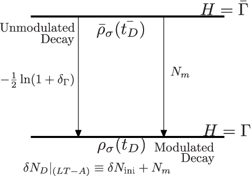
We are going to show obvious correspondences between quantities defined in Ref.[25] and ours in Fig.2. Let us consider the “simplest multi-component Universe” that has been defined in this paper, which is the Universe whose density consists of matter $\rho_{\sigma}$ and radiation $\rho_{r}$ . This model is familiar among the conventional curvaton models. The decay of the matter is therefore looks like a curvaton decay. It is possible to calculate the mixed (modulation-curvaton) perturbations when the curvaton perturbations are not negligible, however in the main part of this paper we have been focusing on the scenario in which modulation is dominating the cosmological perturbation.

In Ref.[25], they have defined the non-linear formalism

\zeta_{\sigma}=\delta N_{D}+\frac{1}{3}\ln\left(\frac{\rho_{\sigma}(t_{D})}{\bar{\rho}_{\sigma}}\right),

(121)

where the hypersurface defined by $t_{D}$ ( $H=\Gamma$ ) is modulated. In that case $\delta N_{D}$ cannot represent the usual curvature perturbation. (See Fig.4.)

In our formalism, these quantities are corresponding to

$\displaystyle\delta N_{D}\|_{(LT-A)}$	$\displaystyle\leftrightarrow$	$\displaystyle\delta N_{\mathrm{ini}}+N_{m}$
$\displaystyle\rho_{\sigma}(t_{D})\|_{(LT-A)}$	$\displaystyle\leftrightarrow$	$\displaystyle\rho_{\sigma,\Gamma,m}=\rho_{\sigma,0}e^{-3N_{m}}$
$\displaystyle\bar{\rho}_{\sigma}(\bar{t}_{D})\|_{(LT-A)}$	$\displaystyle\leftrightarrow$	$\displaystyle\bar{\rho}_{\sigma,0}.$	(122)

We thus find

\zeta_{\sigma}|_{(LT-A)}\leftrightarrow\zeta_{\sigma}.

(123)

They also defined

(1+\delta_{\Gamma})^{2}\equiv\Gamma^{2}/\bar{\Gamma}^{2},

(124)

which gives the correspondence

(1+\delta_{\Gamma})^{2}\leftrightarrow e^{-4N_{\not{m}}}.

(125)

Finally, they have defined the post-decay curvature perturbation

\zeta=\delta N_{D}+\frac{1}{2}\ln(1+\delta_{\Gamma}),

(126)

which corresponds to

\zeta|_{(LT-A)}\leftrightarrow\delta N_{\mathrm{ini}}+N_{m}-N_{\not{m}}.

(127)

In our calculation the curvature perturbation generated by the modulated decay is given by

\delta N_{\mathrm{mod}}\equiv N_{m}-N_{\not{m}}.

(128)

Therefore, the correspondence is obvious between our calculation and Ref.[25].

In finding the curvaton contribution they evaluated

\zeta=\zeta_{r}-\frac{r}{6}\delta_{\Gamma}+\frac{r}{3}S,

(129)

where the first and the last terms are originally given by

\zeta_{r}+\frac{r}{3}S=r\zeta_{\sigma}+(1-r)\zeta_{r}\equiv\delta N_{\mathrm{ini}},

(130)

where $\delta N_{\mathrm{ini}}$ is defined previously in this paper. If the curvaton hypothesis is valid and the component perturbations are constant, one may evaluate the component perturbation at $H=H_{\mathrm{osc}}$ as

\displaystyle\zeta_{\sigma}=\zeta_{\sigma}(t_{\mathrm{osc}})=\delta N_{\mathrm{inf}}+\frac{1}{3}\ln\frac{\rho_{\sigma}(t_{\mathrm{osc}})}{\bar{\rho}_{\sigma}(t_{\mathrm{osc}})},

(131)

where $\delta N_{\mathrm{inf}}$ denotes the curvature perturbation just at the beginning of the oscillation. Substituting the component perturbations (defined at $H_{\mathrm{osc}}$ ) into the above equation (130), one will find

$\displaystyle\zeta_{r}+\frac{r}{3}S$	$\displaystyle=$	$\displaystyle r\zeta_{\sigma}(t_{\mathrm{osc}})+(1-r)\zeta_{r}(t_{\mathrm{osc}})$	(132)
	$\displaystyle=$	$\displaystyle\delta N_{\mathrm{inf}}+\frac{r}{3}\ln\frac{\rho_{\sigma}(t_{\mathrm{osc}})}{\bar{\rho}_{\sigma}(t_{\mathrm{osc}})}$
		$\displaystyle+\frac{1-r}{4}\ln\frac{\rho_{r}(t_{\mathrm{osc}})}{\bar{\rho}_{r}(t_{\mathrm{osc}})}.$

Although a deformation is needed, it is easy to find that the result is consistent with Eq.(115).

Using the above formula, they started perturbation with regard to the perturbation of $S$ . For instance, Langlois and Takahashi considered for the “curvaton perturbation”

S\equiv 3(\zeta_{\sigma}-\zeta_{r})=\frac{2\sigma}{\sigma}-\frac{\delta\sigma^{2}}{\sigma^{2}}+\frac{2}{3}\frac{\delta\sigma^{3}}{\sigma^{3}},

(133)

and for the “inflaton perturbation”

\zeta_{r}=\frac{H}{\dot{\phi}}\delta\phi\simeq\delta N_{\mathrm{inf}}.

(134)

These definitions are based on the usual curvaton hypothesis (i.e, valid when one can disregard $\delta\rho_{r}/\rho_{r}$ ).

References

[1] D. H. Lyth, A. R. Liddle, “The primordial density perturbation: Cosmology, inflation and the origin of structure,” Cambridge, UK: Cambridge Univ. Pr. (2009) 497 p.
[2] M. Sasaki and T. Tanaka, Prog. Theor. Phys. 99, 763 (1998) [gr-qc/9801017].; D. Wands, K. A. Malik, D. H. Lyth and A. R. Liddle, “A New approach to the evolution of cosmological perturbations on large scales,” Phys. Rev. D 62, 043527 (2000) [astro-ph/0003278]; D. H. Lyth and D. Wands, Phys. Rev. D 68, 103515 (2003) [astro-ph/0306498].
[3] T. Matsuda, “Delta-N formalism for the evolution of the curvature perturbations in generalized multi-field inflation,” Phys. Lett. B 682, 163 (2009) [arXiv:0906.2525 [hep-th]]; T. Matsuda, “Elliptic Inflation: Generating the curvature perturbation without slow-roll,” JCAP 0609, 003 (2006) [hep-ph/0606137].
[4] F. Bernardeau and J. -P. Uzan, “NonGaussianity in multifield inflation,” Phys. Rev. D 66, 103506 (2002) [hep-ph/0207295]; L. E. Allen, S. Gupta and D. Wands, “Non-gaussian perturbations from multi-field inflation,” JCAP 0601, 006 (2006) [astro-ph/0509719]; H. Assadullahi, H. Firouzjahi, M. H. Namjoo and D. Wands, “Curvaton and the inhomogeneous end of inflation,” arXiv:1207.7006 [astro-ph.CO].
[5] T. Matsuda, “Modulated Inflation,” Phys. Lett. B 665, 338 (2008) [arXiv:0801.2648 [hep-ph]]; T. Matsuda, “Modulated inflation from kinetic term,” JCAP 0805, 022 (2008) [arXiv:0804.3268 [hep-th]].
[6] T. Moroi, T. Takahashi, “Effects of cosmological moduli fields on cosmic microwave background,” Phys. Lett. B522, 215-221 (2001). [hep-ph/0110096]. D. H. Lyth, D. Wands, “Generating the curvature perturbation without an inflaton,” Phys. Lett. B524, 5-14 (2002). [hep-ph/0110002].
[7] K. Dimopoulos, K. Kohri and T. Matsuda, “The hybrid curvaton,” Phys. Rev. D 85, 123541 (2012) [arXiv:1201.6037 [hep-ph]]; T. Matsuda, “Free light fields can change the predictions of hybrid inflation,” JCAP 1204, 020 (2012) [arXiv:1204.0303 [hep-ph]].
[8] K. Dimopoulos, K. Kohri, D. H. Lyth and T. Matsuda, “The inflating curvaton,” JCAP 1203, 022 (2012) [arXiv:1110.2951 [astro-ph.CO]];
[9] K. Kohri, C. -M. Lin and T. Matsuda, “PBH from the inflating curvaton,” arXiv:1211.2371 [hep-ph].
[10] G. Dvali, A. Gruzinov and M. Zaldarriaga, “A new mechanism for generating density perturbations from inflation,” Phys. Rev. D 69, 023505 (2004) [arXiv:astro-ph/0303591].
[11] D. H. Lyth, “Generating the curvature perturbation at the end of inflation,” JCAP 0511, 006 (2005) [astro-ph/0510443]; F. Bernardeau, L. Kofman and J. -P. Uzan, “Modulated fluctuations from hybrid inflation,” Phys. Rev. D 70, 083004 (2004) [astro-ph/0403315].
[12] S. Enomoto, K. Kohri and T. Matsuda, “Non-Gaussianity in the unified curvaton mechanism : The generalized curvaton mechanism that comprehends modulation at the transition,” arXiv:1210.7118 [hep-ph].
[13] T. Matsuda, “Cosmological perturbations from inhomogeneous preheating and multi-field trapping,” JHEP 0707, 035 (2007) [arXiv:0707.0543 [hep-th]].
[14] T. Matsuda, “Cosmological perturbations from an inhomogeneous phase transition,” Class. Quant. Grav. 26, 145011 (2009). [arXiv:0902.4283 [hep-ph]]; M. Kawasaki, T. Takahashi and S. Yokoyama, “Density Fluctuations in Thermal Inflation and Non-Gaussianity,” JCAP 0912, 012 (2009) [arXiv:0910.3053 [hep-th]].
[15] G. N. Felder, L. Kofman and A. D. Linde, Phys. Rev. D 60, 103505 (1999) [hep-ph/9903350]; T. Matsuda, JCAP 0708, 003 (2007) [arXiv:0707.1948 [hep-ph]].
[16] T. Matsuda, “Topological curvatons,” Phys. Rev. D 72, 123508 (2005) [hep-ph/0509063].
[17] D. H. Lyth, “Can the curvaton paradigm accommodate a low inflation scale?,” Phys. Lett. B 579 (2004) 239 [hep-th/0308110].
[18] K. A. Malik and D. H. Lyth, “A numerical study of non-gaussianity in the curvaton scenario,” JCAP 0609, 008 (2006) [astro-ph/0604387].
[19] M. Zaldarriaga, “Non-Gaussianities in models with a varying inflaton decay rate,” Phys. Rev. D 69, 043508 (2004) [astro-ph/0306006]; T. Suyama and M. Yamaguchi, “Non-Gaussianity in the modulated reheating scenario,” Phys. Rev. D 77 (2008) 023505 [arXiv:0709.2545 [astro-ph]]; K. Kohri, D. H. Lyth and C. A. Valenzuela-Toledo, “Preheating and the non-gaussianity of the curvature perturbation,” JCAP 1002, 023 (2010) [Erratum-ibid. 1009, E01 (2011)] [arXiv:0904.0793 [hep-ph]]; M. Cicoli, G. Tasinato, I. Zavala, C. P. Burgess and F. Quevedo, “Modulated Reheating and Large Non-Gaussianity in String Cosmology,” JCAP 1205, 039 (2012) [arXiv:1202.4580 [hep-th]].
[20] D. H. Lyth, K. A. Malik and M. Sasaki, “A General proof of the conservation of the curvature perturbation,” JCAP 0505, 004 (2005) [astro-ph/0411220];
[21] D. Langlois, F. Vernizzi and D. Wands, “Non-linear isocurvature perturbations and non-Gaussianities,” JCAP 0812, 004 (2008) [arXiv:0809.4646 [astro-ph]].
[22] K. Kohri, C. -M. Lin and T. Matsuda, “Delta-N Formalism for Curvaton with Modulated Decay,” arXiv:1303.2750 [hep-ph].
[23] M. Sasaki, J. Valiviita and D. Wands, “Non-Gaussianity of the primordial perturbation in the curvaton model,” Phys. Rev. D 74, 103003 (2006) [astro-ph/0607627].
[24] M. S. Turner, “Coherent Scalar Field Oscillations in an Expanding Universe,” Phys. Rev. D 28, 1243 (1983).
[25] D. Langlois and T. Takahashi, “Density Perturbations from Modulated Decay of the Curvaton,” arXiv:1301.3319 [astro-ph.CO]; H. Assadullahi, H. Firouzjahi, M. H. Namjoo and D. Wands, “Modulated curvaton decay,” arXiv:1301.3439 [hep-th].

Modulated decay in the multi-component Universe

Abstract

pacs

I Introduction

II Modulated decay in the simple multi-component Universe

II.1 First order

II.2 Second order

II.2.1 Decay rates

II.2.2 fN​Lf_{NL}

III Higher potential or topological defects

III.1 First order

III.2 fN​Lf_{NL}

IV Partial decay

IV.1 First order

IV.2 Second order

V Conclusion and discussion

VI Acknowledgment

Appendix A Non-Linear formalism and the curvaton mechanism

A.1 Why difficult?

A.2 Quantities defined in Ref.[25]

References

II.2.2 $f_{NL}$

III.2 $f_{NL}$