On surface meshes induced by level set functions

Surface triangulations occur in, for example, visualization, shape optimization, surface restoration and in applications where differential equations posed on surfaces are treated numerically. Hence, properties of surface triangulations such as shape regularity and angle conditions are of interest. For example, angle conditions are closely related to approximation properties and stability of corresponding finite elements [1, 2].

In this article, we are interested in the properties of a surface triangulation if one considers the zero level of a continuous piecewise-affine function with respect to a consistent tetrahedral subdivision of a domain in $\mathbb{R}^{3}$. The zero level of a piecewise-affine function is a piecewise-planar hyper-surface consisting of triangles and quadrilaterals. Each quadrilateral can be divided into two triangles in such a way that the resulting surface triangulation satisfies the following property proved in this paper: if the volume tetrahedral subdivision satisfies a minimum angle condition, then the corresponding surface triangulation satisfies a maximum angle condition. We show that the maximum angle occuring in the surface triangulation can be bounded by a constant $\phi_{\max}<\pi$ that depends only on a stability constant for the family of tetrahedral subdivisions.

The paper also discusses a few implications of this property for the numerical solution of surface partial differential equations. Numerical methods for surface PDEs are studied in e.g., [6, 4, 5, 3, 8, 10]. We derive optimal approximation properties of $P_{1}$ finite element functions with respect to the surface triangulation and a uniform bound for the condition number of the scaled mass matrix. We also show that the condition number of the (scaled) stiffness matrix can be very large and is sensitive to the distribution of the vertices of tetrahedra close to the surface. Some numerical examples illustrate the analysis of the paper.

Consider a smooth surface $\Gamma$ in three dimensional space. For simplicity, we assume that $\Gamma$ is connected and has no boundary. Let $\Omega\subset\mathbb{R}^{3}$ be a bulk domain which contains $\Gamma$. Let $\{\mathcal{T}_{h}\}_{h>0}$ be a family of tetrahedral triangulations of the domain $\Omega$. These triangulations are assumed to be regular, consistent and stable, cf. [2]. To simplify the presentation, we assume that this family of triangulations is quasi-uniform. The latter assumption, however, is not essential for our analysis.

We assume that for each $\mathcal{T}_{h}$ an approximation of $\Gamma$, denoted by $\Gamma_{h}$, is given which is a connected $C^{0,1}$ surface without boundary. In our analysis we assume $\Gamma_{h}$ to be consistent with $\mathcal{T}_{h}$ is the sense as explained in the following definition.

If $\Gamma_{h}$ is consistent with $\mathcal{T}_{h}$, then every segment $T=S_{T}\cap\Gamma_{h}$ is either a triangle or a quadrilateral. Each quadrilateral segment can be divided into two triangles, so we may assume that every $T$ is a triangle.

Let $\mathcal{F}_{h}$ be the set of all triangular segments $T$, then $\Gamma_{h}$ can be decomposed as

The most prominent example of such a surface triangulation is obtained in the context of level set techniques. Assume that $\Gamma$ is represented as the zero level of a level set function $\phi$ and that $\phi_{h}$ is a continuous linear finite element approximation on the outer tetrahedral triangulation $\mathcal{T}_{h}$. Then if we define $\Gamma_{h}$ to be the zero level of $\phi_{h}$ then $\Gamma_{h}$ consists of piecewise planar segments and is consistent with $\mathcal{T}_{h}$. As an example, consider a sphere $\Gamma$, represented as the zero level of its signed distance function. For $\phi_{h}$ we take the piecewise linear nodal interpolation of this distance function on a uniform tetrahedral triangulation $\mathcal{T}_{h}$ of a domain that contains $\Gamma$. The zero level of this interpolant defines $\Gamma_{h}$ and is illustrated in Fig. 1.

In the setting of level set methods, such surface triangulations induced by a finite element level set function on a regular outer tetrahedral triangulation are very natural and easy to construct. A surface triangulation $\Gamma_{h}$ that is consistent with the outer triangulation may be the result of another method than the level set method. In the remainder we only need that $\Gamma_{h}$ is consistent with the outer triangulation and not that it is generated by a level set technique.

Note that the triangulation $\mathcal{F}_{h}$ is not necessarily regular, i.e. elements $T\in\mathcal{F}_{h}$ may have very small inner angles and the size of neighboring triangles can vary strongly, cf. Fig. 1. In the next section we prove that, provided each quadrilateral is divided into two triangles properly, the induced surface triangulation is such that the maximal angle condition [1] is satisfied.

The family of outer tetrahedral triangulations $\{\mathcal{T}_{h}\}_{h>0}$ is assumed to be regular, i.e., it contains no hanging nodes and the following stability property holds:

where $\rho(S)$ and $r(S)$ are the diameters of the smallest ball that contains $S$ and the largest ball contained in $S$, respectively. The stability property implies that the family of tetrahedral triangulations satisfies a minimum (and thus also maximum) angle condition: there exists $\theta_{\min}>0$ with

such that all inner angles of all sides of $S\in\mathcal{T}_{h}$ and all angles between edges of $S$ and their opposite side are in the interval $[\theta_{\min},\pi-\theta_{\min}]$. The constant $c(\alpha)$ depends only on $\alpha$ from (2).

Although the surface mesh $\Gamma_{h}$ induced by $\mathcal{T}_{h}$ can be highly shape irregular, the following lemma shows that a maximum angle property holds.

The lemma readily yields the following result.

In the remainder we assume that quadrilaterals are subdivided in the way as explained in Theorem 3. Hence, the inner angles in the surface triangulation $\mathcal{F}_{h}$ are bounded by a constant $\theta^{\ast}<\pi$ that depends only on the stability (close to $\Gamma$) of the outer tetrahedral triangulation $\mathcal{T}_{h}$. In particular $\theta^{\ast}$ is independent of $h$ and of how $\Gamma_{h}$ intersects the outer triangulation $\mathcal{T}_{h}$.

In this section, we use the maximum angle property of the surface triangulation to derive an optimal finite element interpolation result. On $\mathcal{F}_{h}$ we consider the space of linear finite element functions:

This finite element space is the same as the one studied by Dziuk in [5], but an important difference is that in the approach in [5] the triangulations have to be shape regular. In general, the finite element space $V_{h}$ is different from the surface finite element space constructed in [8, 9].

Below we derive an approximation result for the finite element space $V_{h}$. Since the discrete surface $\Gamma_{h}$ varies with $h$, we have to explain in which sense $\Gamma_{h}$ is close to $\Gamma$. For this we use a standard setting applied in the analysis of discretization methods for partial differential equations on surfaces, e.g. [4, 5, 6, 7, 9].

Let $U:=\{\,x\in\mathbb{R}^{3}~|~{\rm dist}(x,\Gamma)<c\,\}$ be a sufficiently small neighborhood of $\Gamma$. We define $\mathcal{T}_{h}^{\Gamma}:=\{\,T\in\mathcal{T}_{h}~|~{\rm meas}_{2}(T\cap\Gamma_{h})>0\,\}$, i.e., the collection of tetrahedra which intersect the discrete surface ${\Gamma}_{h}$, and assume that $\mathcal{T}_{h}^{\Gamma}\subset U$. Let $d$ be the signed distance function to $\Gamma$, with $d<0$ in the interior of $\Gamma$,

Thus $\Gamma$ is the zero level set of $d$. Note that $\mathbf{n}_{\Gamma}=\nabla d$ on $\Gamma$. We define $\mathbf{n}(x):=\nabla d(x)$ for $x\in U$. Thus $\mathbf{n}$ is the outward pointing normal on $\Gamma$ and $\|\mathbf{n}(x)\|=1$ for all $x\in U$. Here and in the remainder $\|\cdot\|$ denotes the Euclidean norm on $\mathbb{R}^{3}$. We introduce a local orthogonal coordinate system by using the projection $\mathbf{p}:\,U\rightarrow\Gamma$:

We assume that the decomposition $x=\mathbf{p}(x)+d(x)\mathbf{n}(x)$ is unique for all $x\in U$. Note that $\mathbf{n}(x)=\mathbf{n}\big(\mathbf{p}(x)\big)$ for all $x\in U$. For a function $v$ on $\Gamma$, its extension is defined as

The outward pointing (piecewise constant) unit normal on $\Gamma_{h}$ is denoted by $\mathbf{n}_{h}$. Using this local coordinate system we introduce the following assumptions on $\Gamma_{h}$:

where $h=\sup_{T\in\mathcal{T}_{h}^{\Gamma}}\rho(T)$. In (12)-(13) we use the common notation, that the inequality holds with a constant independent of $h$. In (13), only $x\in\Gamma_{h}$ are considered for which $\mathbf{n}_{h}(x)$ is well-defined. Using these assumptions, the following result is derived in [5].

In this section we present a few results of numerical experiments which illustrate the interpolation estimates from Theorem 5 and the conditioning of mass and stiffness matrices. Assume the surface $\Gamma$, which is the unit sphere $\Gamma=\{\,x\in\mathbb{R}^{3}~|~\|x\|=1\,\}$, is embedded in the bulk domain $\Omega=[-2,2]^{3}$. The signed distance function to $\Gamma$ is denoted by $d$. We construct a hierarchy of uniform tetrahedral triangulations $\{\mathcal{T}_{h}\}$ for $\Omega$, with $h\in\{1/2,1/4,1/8,1/16,1/32\}$. Let $d_{h}$ be the piecewise nodal Lagrangian interpolant of $d$. The triangulated surface is given by

The corresponding finite element space $V_{h}$ consists of all piecewise affine functions with respect to $\mathcal{F}_{h}$, as defined in (9). For $h\in\{1/2,1/4,1/8,1/16,1/32\}$, the resulting dimensions of $V_{h}$ are $N=164,812,3500,14264,57632$, respectively. In agreement with the 2D nature of $\Gamma_{h}$, we have $N\sim h^{-2}$.

To illustrate the result of Theorem 5, we present the interpolation errors $\|u^{e}-I_{h}u^{e}\|_{L^{2}(\Gamma_{h})}$ and $|u^{e}-I_{h}u^{e}|_{1,\Gamma_{h}}$ for the smooth function

defined on the unit sphere, with $x=(x_{1},x_{2},x_{3})^{T}$. The dependence of the interpolation errors on the number of degrees of freedom $N$ is shown in Figure 4 (left). We observe the optimal error reduction behavior, consistent with the estimates in (18), (19).

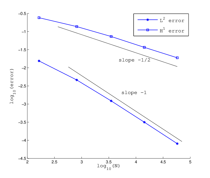
Further, for the same sequence of meshes we compute the spectral condition numbers of the mass matrix $\mathbf{M}$ and the diagonally scaled mass matrix $\mathbf{M}^{s}$. The dependence of the condition numbers on the number of degrees of freedom $N$ is illustrated in Figure 4 (right). As was proved in Theorem 6, the scaled mass matrix has a uniformly bounded condition number.

We discussed in section 4.3 that concerning the effective condition number of the scaled stiffness matrix the situation is more delicate. To illustrate this, we performed an experiment in which the intersection between a fixed outer triangulation and the surface is varied. Let $\Gamma$ be the boundary of the unit sphere with the center located in $(0,0,z_{c})$. The discrete surface $\Gamma_{h}$ is defined as described above, induced by the uniform outer triangulation. We choose a fixed outer triangulation with $h=1/16$. We now consider different values for $z_{c}$, thus “moving the surface through the outer triangulation”. The $z_{c}$ values are given in the first column of Table 1. Note that for the largest shift $z_{c}=0.03$ we have $z_{c}\approx 0.5h$.

For the different surface triangulations we computed the interpolation errors as described above. It turns out that for the values $z_{c}\neq 0$ the error behavior is essentially the same as that for $z_{c}=0$ (illustrated in Fig. 4).

In the second to fourth columns of Table 1 two geometry related quantities are given. The second column shows the value of the maximum angle occuring in the surface triangulation. Consistent to the theory, cf. Theorem 3, the maximum angle is bounded away from $180^{\circ}$. Small angles, however, can occur. In the third and fourth column we show the value of the minimum angle and the number of triangles in the surface triangulation with the smallest angle smaller than $1^{\circ}$. As expected, both the minimal angle and this number of small angles strongly varies depending on $z_{c}$. For $z_{c}=0$ the smallest angle in the surface triangulation has value $\phi_{\rm min}=1.85^{\circ}$. Extremely small angles can occur, e.g. for $z_{c}=0.00005$, we have $\phi_{\rm min}=8.54$e-$7^{\circ}$. The dimension and the effective condition number of the scaled stiffness matrix $\mathbf{A}^{s}$ are given in the fifth and sixth column of Table 1. The values of the condition number show a strong dependence on the sphere location (value of $z_{c}$). These large condition numbers indicate that linear systems with these matrices may be hard to solve using an iterative method. To investigate this further, we used the standard PCG MATLAB solver with ILU(0) preconditioner. For given $\mathbf{v}$, we computed $\mathbf{b}=\mathbf{A}^{s}\mathbf{v}$ and applied the MATLAB PCG iterative solver with a relative residual tolerance of $10^{-8}$. The resulting iteration numbers are given in column 7 of Table 1. These iteration counts are “high” compared to the ones that are generally needed for standard discretization of diffusion problems. To make this more quantitative, we constructed a reference matrix $\mathbf{A}^{\rm ref}$ as follows: $\mathbf{A}^{\rm ref}={\rm blocktridiag}(-\mathbf{B}^{T},\mathbf{D},-\mathbf{B})$, with $\mathbf{D}={\rm tridiag}(-1,6,-1)$, $\mathbf{B}={\rm tridiag}(0,1,1)$. In most rows the matrix $\mathbf{A}^{\rm ref}$ has 7 nonzero entries, which is approximately the same as the average number of nonzero entries per row in the matrix $\mathbf{A}^{s}$ used in the experiment. In $\mathbf{A}^{\rm ref}$ we use 120 blockrows and blockcolums and the matrices $\mathbf{D}$ and $\mathbf{B}$ have dimension 120. Then the matrix $\mathbf{A}^{\rm ref}$ has dimension 14400, which is comparable to the dimension of $\mathbf{A}^{s}$ used in the experiment, cf. Table 1. The same iterative solver with the same stopping criterion applied to a linear system with $\mathbf{A}^{\rm ref}$ resulted in 42 PCG iterations, which is much lower than the iteration numbers listed in Table 1.
In view of these observations, and the fact that solving a PDE on a surface (in 3D) is a two-dimensional problem, it is better to use a direct solver. We performed experiments with the MATLAB sparse direct solver $\mathbf{A}^{s}\setminus\mathbf{b}$. We measured computing time by the MATLAB function cputime. For the system with the reference matrix $\mathbf{A}^{\rm ref}$ we obtained (on our machine) cputime$=1.38$. For the matrix $\mathbf{A}^{s}$ we obtained CPU time measurements given in the last column of Table 1. These show that for the direct MATLAB solver the matrices $\mathbf{A}^{s}$ are not (much) more difficult to deal with than the reference matrix $\mathbf{A}^{\rm ref}$. Variations in CPU times are probably caused by slightly different fill-in properties of matrices for different grids. The one dimensional kernel of the matrix $\mathbf{A}^{s}$ did not cause difficulties for the solver. We checked the accuracy of the computed solution (in the energy norm) and this was satisfactory.

The main new result of this paper is a geometric property of the piecewise planar surface which is the zero level of a continuous piecewise affine level set function. If this piecewise planar surface is consistent with an outer tetrahedral triangulation that satisfies the minimum angle condition, then after a suitable subdivision of the quadrilaterals into two triangles the resulting surface triangulation satisfies a maximum angle condition. This maximum angle property of the surface triangulation is used to derive optimal error bounds for the nodal interpolation operator in the finite element space of continuous piecewise linear functions on the surface triangulation. This implies that the discretization of a surface diffusion PDE in this finite element space results in optimal discretization error bounds. We study the conditioning of the scaled mass and stiffness matrices corresponding to this finite element space. The condition number of the scaled mass matrix is shown to be uniformly bounded. The scaled stiffness matrix can have a very large effective condition number. Results of a numerical experiment indicate that for solving systems with the scaled stiffness matrix it is better to use a sparse direct solver rather than an iterative solver. A topic that we plan to investigate further is whether some grid smoothing (elimination of extremely small angles) can be developed such that the optimal approximation property still holds and the conditioning of the scaled stiffness matrix is improved.

The authors thank the referees for their comments, which have led to significant improvements of the original version of this paper. This work has been supported in part by the DFG through grant RE1461/4-1 and the Russian Foundation for Basic Research through grants 12-01-91330, 12-01-00283.

References

- [1] I. Babuška and A. K. Aziz. On the angle condition in the finite element method. SIAM J. Numer. Anal., 13:214–226, 1976.
- [2] P. Ciarlet. The Finite Element Method for Elliptic Problems. North-Holland, Amsterdam, 1978.
- [3] A. Demlow. Higher-order finite element methods and pointwise error estimates for elliptic problems on surfaces. SIAM J. Numer. Anal., 47:805–827, 2009.
- [4] A. Demlow and G. Dziuk. An adaptive finite element method for the Laplace-Beltrami operator on implicitly defined surfaces. SIAM J. Numer. Anal., 45:421–442, 2007.
- [5] G. Dziuk. Finite elements for the Beltrami operator on arbitrary surfaces. In S. Hildebrandt and R. Leis, editors, Partial differential equations and calculus of variations, volume 1357 of Lecture Notes in Mathematics, pages 142–155. Springer, 1988.
- [6] G. Dziuk and C. Elliott. Finite elements on evolving surfaces. IMA J. Numer. Anal., 27:262–292, 2007.
- [7] G. Dziuk and C. Elliott. -estimates for the evolving surface finite element method. Math. Comp., 82:1–24, 2013.
- [8] M. A. Olshanskii and A. Reusken. A finite element method for surface PDEs: matrix properties. Numer. Math., 114:491–520, 2009.
- [9] M. A. Olshanskii, A. Reusken, and J. Grande. A finite element method for elliptic equations on surfaces. SIAM J. Numer. Anal., 47:3339–3358, 2009.
- [10] J.-J. Xu and H.-K. Zhao. An Eulerian formulation for solving partial differerential equations along a moving interface. J. Sci. Comput., 19:573–594, 2003.