跳到论文正文
W Papers独立论文阅读器 arXiv:1301.3642 论文正文 计算阅读时间 · 0%
引用这篇论文根据当前论文元数据生成,正式投稿前建议核对。


License: arXiv.org perpetual non-exclusive license
arXiv:1301.3642v2 [cond-mat.quant-gas] 11 Oct 2013

Fluctuation-induced and symmetry-prohibited metastabilities in spinor Bose-Einstein condensates

Preprint: APS/123-QED
Nguyen Thanh Phuc Affiliation: Department of Physics, University of Tokyo, 7-3-1 Hongo, Bunkyo-ku, Tokyo 113-0033, Japan    Yuki Kawaguchi Affiliation: Department of Applied Physics and Quantum-Phase Electronics Center, University of Tokyo, 2-11-6 Yayoi, Bunkyo-ku, Tokyo 113-0032, Japan    Masahito Ueda Affiliation: Department of Physics, University of Tokyo, 7-3-1 Hongo, Bunkyo-ku, Tokyo 113-0033, Japan
August 24, 2026
Abstract

Spinor Bose-Einstein condensates provide a unique example in which the Bogoliubov theory fails to describe the metastability associated with first-order quantum phase transitions. This problem is resolved by developing the spinor Beliaev theory which takes account of quantum fluctuations of the condensate. It is these fluctuations that generate terms of higher than the fourth order in the order-parameter field which are needed for the first-order phase transitions. Besides the conventional first-order phase transitions which are accompanied by metastable states, we find a class of first-order phase transitions which are not accompanied by metastable states. The absence of metastability in these phase transitions holds to all orders of approximation since the metastability is prohibited by the symmetry of the Hamiltonian at the phase boundary. Finally, the possibility of macroscopic quantum tunneling from a metastable state to the ground state is discussed.

pacs
03.75.Mn,03.75.Kk,67.85.Jk

I Introduction

Quantum phase transitions have been an active field of research in solid-state materials such as magnetic insulators, heavy fermions, semiconductors, and high-temperature superconductors [1, 2]. In ultracold atoms, the superfluid–Mott-insulator phase transition has been investigated both theoretically and experimentally [3, 4]. While many of these studies focus on the second-order or continuous quantum phase transitions due to their criticality, the first-order quantum phase transitions in fermionic systems such as itinerant electron magnets [5] and superfluid helium-3 [6] have attracted considerable attention in connection with non–Fermi-liquid phases and superconductivity [7, 8]. In bosonic systems, first-order quantum phase transitions appear in various Bose-Einstein condensates (BECs) with special interatomic interactions such as soft-core [9, 10] and dipole-dipole [11] interactions, or under external potentials with special geometries [12]. The metastability associated with the first-order phase transitions in these systems can be explained at the mean-field level by using the Bogoliubov theory [13].

In the present study, we point out a special feature of spinor BECs [14] in which metastable states are induced by quantum fluctuations. In spinor BECs, there exist several ground-state phases with different invariant symmetries, implying a discontinuity in the order parameter space at the phase boundaries; therefore, the phase transitions should be first order. The conventional wisdom suggests that there appear metastable states around the phase boundaries. However, the Bogoliubov analysis shows no metastable state for all of these phase transitions. Such an inconsistency arises because the Bogoliubov theory relies on the Gross-Pitaevskii energy functional, which, in the case of a homogeneous system with a contact interaction, is equivalent to Landau’s ϕ2+ϕ4\phi^{2}+\phi^{4} model of continuous phase transitions, whereas a first-order quantum phase transition requires higher-order terms in ϕ\phi. In this paper, we resolve this problem by developing the spinor Beliaev theory for spin-2 BECs [15, 16, 17, 18], which takes account of higher-order terms beyond ϕ4\phi^{4} due to the quantum depletion of the condensate. After obtaining the ground-state phase diagram of spin-2 BECs at the level of the Lee-Huang-Yang correction [19, 20], we examine in detail the possibility of metastable states associated with the first-order phase transitions and show that the metastability indeed arises from quantum fluctuations.

Besides the first-order phase transitions with fluctuation-induced metastability, we also find in spinor BECs a class of first-order phase transitions that have no metastable state around the phase boundary. We show that in this case the absence of metastability holds to all orders of approximation. This appears to be contrary to the conventional wisdom that every first-order phase transition is associated with a metastable state, but in fact there are other examples of this kind of phase transitions such as the ferromagnetic X​X​ZXXZ spin model in which a level crossing occurs as the anisotropy of the interaction is varied [21]. Such phase transitions are characterized by the fact that the Hamiltonian acquires a special symmetry at the phase boundary so that the energy landscape becomes flat. The ground state would then abruptly change to an unstable state without undergoing any transient regime of metastability as the system crosses the phase boundary. This is in contrast to the case of conventional first-order phase transitions where the energy landscape features a double well at the transition point, leading to the coexistence of two phases. In this paper, we explicitly investigate the symmetries of the Hamiltonians that underlie the flat energy landscapes in spin-1 and spin-2 BECs. The high symmetry of the Hamiltonian at the phase boundary prohibits the metastability to all orders of approximation. Finally, the time scale of a macroscopic quantum tunneling (MQT) from a metastable state to the ground state is estimated for the case of cyclic-uniaxial nematic phase transition as it is relevant to experiments of the spin-2 Rb87{}^{\text{87}}\text{Rb} BEC.

This paper is organized as follows. Section II derives the ground-state phase diagram at the level of the Lee-Huang-Yang correction. Section III develops the spinor Beliaev theory for spin-2 BECs. The fluctuation-induced metastabilities of first-order quantum phase transitions that cannot be captured by the Bogoliubov theory are discussed in Sec. III.1. The general formalism of the spinor Beliaev theory is developed in Sec. III.2, based on which the stability analyses of the ferromagnetic and uniaxial-nematic phases are carried out in Sec. III.3. Section IV introduces the first-order quantum phase transitions that are not accompanied by metastable states to all orders of approximations. The underlying symmetry of the Hamiltonian that prohibits the metastability is discussed for both spin-1 and spin-2 BECs. Section V estimates the rate of MQT near the cyclic-uniaxial nematic phase boundary. Section VI concludes this paper. Some detailed calculations are relegated to the Appendices to avoid digressing from the main subject. Note that in contrast to Refs. [22, 23, 24, 25], in this paper we do not make the single-mode approximation (SMA). Consequently, the coupling between the spin and the motional degrees of freedom of atoms is not neglected, and we investigate the effect of quantum depletion of the condensate on the phase diagram and phase transitions.

II Beyond-mean-field ground-state phase diagram of spin-2 BECs

We consider a homogeneous BEC of spin-2 atoms with mass MM and described by the field operator ψ^j\hat{\psi}_{j}, where j=2,⋯,−2j=2,\cdots,-2 denotes the magnetic quantum number. The second-quantized Hamiltonian of the system is given by H^=h^0+V^\hat{H}=\hat{h}_{0}+\hat{V}, where

h^0=∫d​𝐫​∑j=−22ψ^j†​(𝐫)​(−ℏ2​∇22​M)​ψ^j​(𝐫)\displaystyle\hat{h}_{0}=\int\text{d}\mathbf{r}\sum_{j=-2}^{2}\hat{\psi}^{\dagger}_{j}(\mathbf{r})\left(-\frac{\hbar^{2}\nabla^{2}}{2M}\right)\hat{\psi}_{j}(\mathbf{r}) (1)

is the kinetic energy and

V^=12∫d𝐫[\displaystyle\hat{V}=\frac{1}{2}\int\text{d}\mathbf{r}\Big[ c0:n^2:+c1:𝐅^2:+c2:A^00†A^00:]\displaystyle c_{0}:\hat{n}^{2}:+c_{1}:\hat{\mathbf{F}}^{2}:+c_{2}:\hat{A}_{00}^{\dagger}\hat{A}_{00}:\Big] (2)

is the contact interaction energy [26, 27]. Here :⁣::: denotes normal ordering of operators; i.e., the creation operators are placed to the left of the annihilation operators, and n^≡∑jψ^j†​(𝐫)​ψ^j​(𝐫)\hat{n}\equiv\sum_{j}\hat{\psi}^{\dagger}_{j}(\mathbf{r})\hat{\psi}_{j}(\mathbf{r}), 𝐅^≡∑i,jψ^i†​(𝐫)​(𝐟)i​j​ψ^j​(𝐫)\hat{\mathbf{F}}\equiv\sum_{i,j}\hat{\psi}^{\dagger}_{i}(\mathbf{r})(\mathbf{f})_{ij}\hat{\psi}_{j}(\mathbf{r}), and A^00≡(1/5)​∑j(−1)−j​ψ^j​(𝐫)​ψ^−j​(𝐫)\hat{A}_{00}\equiv(1/\sqrt{5})\sum_{j}(-1)^{-j}\hat{\psi}_{j}(\mathbf{r})\hat{\psi}_{-j}(\mathbf{r}) are the number density, the spin density, and the spin-singlet-pair amplitude operators, respectively, where (𝐟)i​j(\mathbf{f})_{ij} denotes the i​jij component of the spin-2 matrix vector. The coefficients c0,c1c_{0},c_{1}, and c2c_{2} are related to the ss-wave scattering lengths aℱa_{\mathcal{F}} (ℱ=0,2,4\mathcal{F}=0,2,4) of the total spin-ℱ\mathcal{F} channel by c0=4​π​ℏ2​(4​a2+3​a4)/(7​M)c_{0}=4\pi\hbar^{2}(4a_{2}+3a_{4})/(7M), c1=4​π​ℏ2​(a4−a2)/(7​M)c_{1}=4\pi\hbar^{2}(a_{4}-a_{2})/(7M), and c2=4​π​ℏ2​(7​a0−10​a2+3​a4)/(7​M)c_{2}=4\pi\hbar^{2}(7a_{0}-10a_{2}+3a_{4})/(7M), respectively. The order parameter is represented by the five-component spinor ϕ=n0​(ξ2,ξ1,ξ0,ξ−1,ξ−2)T\bm{\phi}=\sqrt{n_{0}}(\xi_{2},\xi_{1},\xi_{0},\xi_{-1},\xi_{-2})^{\mathrm{T}}, where n0n_{0} is the number density of condensate atoms, T denotes transpose, and ξj\xi_{j}’s are normalized to unity; i.e., ∑j=−22|ξj|2=1\sum_{j=-2}^{2}|\xi_{j}|^{2}=1.

The ground-state phase diagram with the Lee-Huang-Yang (LHY) correction is shown in Fig. 1. The LHY correction is the leading-order correction to the Hartree mean-field energy, which arises from quantum depletion of the condensate [19, 20]. Recent experiments on ultracold atoms have demonstrated that the LHY correction can accurately account for the deviation from the Hartree energy up to the strongest interaction realized to date [28]. At the Hartree mean-field level, three phases exist for spin-2 BECs, namely, ferromagnetic, cyclic, and nematic phases whose order parameters are given by 𝝃FM=(1,0,0,0,0)T\bm{\xi}^{\mathrm{FM}}=(1,0,0,0,0)^{\mathrm{T}}, 𝝃CL=(1,0,0,2,0)T/3\bm{\xi}^{\mathrm{CL}}=(1,0,0,\sqrt{2},0)^{\mathrm{T}}/\sqrt{3}, and 𝝃NM​(η)=(sin⁡η/2,0,cos⁡η,0,sin⁡η/2)T\bm{\xi}^{\mathrm{NM}}(\eta)=(\sin\eta/\sqrt{2},0,\cos\eta,0,\sin\eta/\sqrt{2})^{\mathrm{T}}, respectively, where the parameter η\eta characterizes the nematicity in the ground-state manifold of the nematic phase [29]. At the Hartree mean-field level, the nematic phases having different values of η\eta are degenerate. Note that the ground-state manifold of each phase contains all states obtained by letting an SO(3) rotational operator U⁡(α,β,γ)=e−i​fz​α​e−i​fy​β​e−i​fz​γU(\alpha,\beta,\gamma)=e^{-if_{z}\alpha}e^{-if_{y}\beta}e^{-if_{z}\gamma} act on a representative order parameter. Here, α\alpha, β\beta, and γ\gamma denote the Euler angles of a rotation in spin space. For example, the order parameter (1,0,i2,0,1)T/2=U(π/3,arccos(−1/3),−π/3)(1/3,0,0,2/3,0)T(1,0,i\sqrt{2},0,1)^{\mathrm{T}}/2=U(\pi/3,\arccos(-1/\sqrt{3}),-\pi/3)(1/\sqrt{3},0,0,\sqrt{2/3},0)^{\mathrm{T}} also represents one state in the ground-state manifold of the cyclic phase. The LHY correction to the mean-field ground-state energy are calculated in Refs. [30, 31, 32]. With the LHY corrections, the phase boundaries are modified as follows. The detailed calculations are given in Appendix A.

Uniaxial nematic (UN) - biaxial nematic (BN) phase boundary. As shown in Refs. [30, 31], zero-point fluctuations lift the degeneracy in the nematic phase, rendering the ground states UN (η=n​π/3\eta=n\pi/3) and BN (η=π/6+n​π/3\eta=\pi/6+n\pi/3) for c1>0c_{1}>0 and c1<0c_{1}<0, respectively. Therefore, the UN-BN phase transition occurs at c1=0c_{1}=0. Note that all states whose order parameters are given by different values of n=0,…,5n=0,\dots,5 are energy degenerate and belong to the same ground-state manifold; especially, the BN phase includes states with order parameters (2,0,2​3,0,2)T/4(\sqrt{2},0,2\sqrt{3},0,\sqrt{2})^{\mathrm{T}}/4 (η=π/6\eta=\pi/6) and (1,0,0,0,1)T/2(1,0,0,0,1)^{\mathrm{T}}/\sqrt{2} (η=π/2\eta=\pi/2).

Ferromagnetic-BN phase boundary. By comparing the ground-state energies with the LHY corrections of the ferromagnetic and BN phases [see Eqs. (46)-(48) in Appendix A], we find that the ferromagnetic-BN phase boundary is shifted from its mean-field counterpart of c2=20​c1c_{2}=20c_{1} [26] to

c2FM−BN≃\displaystyle c_{2}^{\mathrm{FM-BN}}\simeq  20​c1−1521​(|c1|c0)3/2​n​a3​|c1|;\displaystyle\,20c_{1}-1521\left(\frac{|c_{1}|}{c_{0}}\right)^{3/2}\sqrt{na^{3}}\,|c_{1}|; (3)

i.e., the region of the ferromagnetic phase is enlarged.

UN-cyclic phase boundary. Similarly, the phase boundary between the UN and cyclic phases is given by [see Eqs. (49)–(51) in Appendix A]

c2UN−CL≃\displaystyle c_{2}^{\mathrm{UN-CL}}\simeq −342​(c1c0)3/2​n​a3​c1.\displaystyle\,-342\left(\frac{c_{1}}{c_{0}}\right)^{3/2}\sqrt{na^{3}}\,c_{1}. (4)

Compared with the mean-field UN-cyclic phase boundary of c1>0,c2=0c_{1}>0,c_{2}=0 [26], the region of the cyclic phase is enlarged.

Ferromagnetic-cyclic phase boundary. The LHY correction does not shift the ferromagnetic-cyclic phase boundary. Actually, this phase boundary stays at c1=0c_{1}=0 to all orders of approximation. From the order parameters 𝝃FM=(1,0,0,0,0)T\bm{\xi}^{\mathrm{FM}}=(1,0,0,0,0)^{\mathrm{T}} and 𝝃CL=(1,0,0,2,0)T/3\bm{\xi}^{\mathrm{CL}}=(1,0,0,\sqrt{2},0)^{\mathrm{T}}/\sqrt{3}, it is evident that the ground-state energies of the ferromagnetic and cyclic phases are independent of c2c_{2} since the excitations caused by c2c_{2} vanish due to the absence of spin-singlet pairs in both of these phases. Because c0c_{0} is the coupling constant of a spin-independent interaction, the energies of these two phases are equal at c1=0c_{1}=0; i.e., the phase boundary is not shifted by quantum fluctuations.

Refer to caption
Figure 1: (Color online) Ground-state phase diagram of spin-2 BECs obtained with the LHY correction. The dashed lines indicate the phase boundaries obtained with the Hartree mean-field approximation. The representative order parameters of the ferromagnetic, cyclic, uniaxial-nematic (UN), and biaxial-nematic (BN) phases are given by 𝝃FM=(1,0,0,0,0)T\bm{\xi}^{\mathrm{FM}}=(1,0,0,0,0)^{\mathrm{T}}, 𝝃CL=(1,0,0,2,0)T/3\bm{\xi}^{\mathrm{CL}}=(1,0,0,\sqrt{2},0)^{\mathrm{T}}/\sqrt{3}, 𝝃UN=(0,0,1,0,0)T\bm{\xi}^{\mathrm{UN}}=(0,0,1,0,0)^{\mathrm{T}}, and 𝝃BN=(2,0,2​3,0,2)T/4\bm{\xi}^{\mathrm{BN}}=(\sqrt{2},0,2\sqrt{3},0,\sqrt{2})^{\mathrm{T}}/4, respectively. The inset in each phase shows the surface plot of |ψ⁡(θ,ϕ)|2≡|∑m=−22ξm​Y2m​(θ,ϕ)|2|\psi(\theta,\phi)|^{2}\equiv|\sum_{m=-2}^{2}\xi_{m}Y^{m}_{2}(\theta,\phi)|^{2}, where Y2mY^{m}_{2}’s are the spherical harmonic functions of rank 2 and the hue indicates the phase of ψ⁡(θ,ϕ)\psi(\theta,\phi) according to the color gauge on the right. Note that the ground-state manifold of each phase includes all states obtained by applying SO(3) rotations in spin space to the representative order parameter; e.g., the order parameters 𝝃BN=(1,0,0,0,1)T/2\bm{\xi}^{\mathrm{BN}}=(1,0,0,0,1)^{\mathrm{T}}/\sqrt{2} and 𝝃CL=(1,0,i​2,0,1)T/2\bm{\xi}^{\mathrm{CL}}=(1,0,i\sqrt{2},0,1)^{\mathrm{T}}/2 belong to the BN and cyclic phases, respectively. The LHY correction due to quantum fluctuations lifts the degeneracy in the manifold of the nematic phases, rendering the ground state UN and BN for c1>0c_{1}>0 and c1<0c_{1}<0, respectively. Quantum fluctuations also shift the cyclic-UN and ferromagnetic-BN phase boundaries as indicated by solid lines. However, the ferromagnetic-cyclic phase boundary is not affected to all orders of approximation (see text).

In the presence of an external magnetic field, the difference in the LHY correction among different ground-state phases is of the order of Δ​E≡M3/2​c15/2​n3/2/π2​ℏ3\Delta E\equiv M^{3/2}c_{1}^{5/2}n^{3/2}/\pi^{2}\hbar^{3} (see Appendix A), and it can compete with the quadratic Zeeman energy qBq_{B}. The phase diagram, therefore, depends on the relative strength of these two effects. In the limit of high magnetic field qB≫Δ​Eq_{B}\gg\Delta E, the effect of quantum fluctuations can be ignored, and the ground-state phase diagram is obtained by the Hartree mean-field theory [33]. This is the case in the experiments of a spin-2 Rb87{}^{\text{87}}\text{Rb} BEC described in Ref. [34]. For Rb87{}^{\text{87}}\text{Rb} under a high magnetic field, the BN phase becomes the ground state, while the dynamics starting from the unstable UN phase would populate all magnetic sublevels. In the opposite limit of low magnetic field qB≪Δ​Eq_{B}\ll\Delta E, quantum fluctuations dominate, and the quadratic Zeeman energy becomes negligible. In this case, the ground-state phase diagram is shown in Fig. 1. The crossover between these two distinct regimes occurs at qB∼Δ​Eq_{B}\sim\Delta E, which corresponds to a magnetic field of the order of 7 mG for the parameters of Rb87{}^{\text{87}}\text{Rb} [35, 36] with atomic density n=1015​cm−3n=10^{15}\,\mathrm{cm}^{-3}. All these regimes can, in principle, be investigated since the lowest magnetic field that has been achieved in a controllable manner in ultracold atomic experiments is as small as 0.1 mG [37].

III Spin-2 Beliaev theory

III.1 Fluctuation-induced metastable states

Since the order parameters and the associated symmetries of different phases in Fig. 1 are not continuously transformed at the phase boundary, we may expect that the phase transitions between these phases must be first order. This can be confirmed by a finite jump in the first derivative of the ground-state energy with respect to the parameter that drives the transition at the phase boundary (see Appendix B). First-order phase transitions are usually accompanied by metastable states. However, the Bogoliubov theory predicts either dynamical instability (complex excitation energy) or Landau instability (negative excitation energy) at the mean-field phase boundaries as listed in Appendix C. This implies no metastability. Such an inconsistency is due to the fact that the Bogoliubov spectrum is obtained by linearizing the Gross-Pitatevskii energy functional which, for a homogeneous system with contact interactions, involves only terms up to the fourth order in the order parameter [38]. Here we note that the Gross-Pitaevskii energy functional is equivalent to that of Landau’s ϕ2+ϕ4\phi^{2}+\phi^{4} model. However, to describe the first-order phase transitions, terms of higher orders in ϕ\phi are needed [39], and in gaseous BECs, higher-order terms can only be obtained by taking into account quantum fluctuations. In other words, in the system under consideration, the metastability, if it exists, is induced by quantum fluctuations. In Sec. III.3, we analytically show that metastable states indeed appear as we go to the next-order approximation, i.e., the spinor Beliaev theory [15, 16, 17]. First-order phase transitions in spinor systems have also been investigated by numerically diagonalizing an effective Hamiltonian [40, 41].

The failure of the Bogoliubov theory leads to the disagreement with the ground-state phase diagram (Fig. 1) obtained in Sec. II. For example, the ground state is the ferromagnetic phase for c2>c2F−BNc_{2}>c_{2}^{\mathrm{F-BN}} and c1<0c_{1}<0 [see Eq. (3)], whereas the Bogoliubov spectrum indicates an instability of the ferromagnetic phase for c2F−BN<c2<20​c1c_{2}^{\mathrm{F-BN}}<c_{2}<20c_{1} (see Appendix C).

In the following sections, by using the spinor Beliaev theory, we show that the fluctuation-induced metastable states exist around the ferromagnetic-BN and UN-cyclic phase boundaries (Sec. III.3). At the other two phase boundaries, we find no metastability. We show in Sec. IV that this absence of metastability holds to all orders of approximation since it is prohibited by the high symmetry of the Hamiltonian at the phase boundary. Therefore, the spinor Beliaev theory gives a fully consistent result for each of the four first-order phase transitions in Fig. 1.

III.2 Formalism

In this section, we develop the spinor Beliaev theory for spin-2 BECs based on the Green’s function formalism, and apply it to calculate the excitation energies of the ferromagnetic and UN states. The formalism shares many similarities with the spin-1 Beliaev theory developed in Ref. [17]. From the obtained excitation energies, we can determine the points in the phase diagram at which instabilities set in.

The Dyson equation for the Green’s functions is given by

Gj​j′α​β​(p)=(G0)j​j′α​β​(p)+(G0)j​mα​γ​Σm​m′γ​δ​(p)​Gm′​j′δ​β​(p),\displaystyle G^{\alpha\beta}_{jj^{\prime}}(p)=(G^{0})^{\alpha\beta}_{jj^{\prime}}(p)+(G^{0})^{\alpha\gamma}_{jm}\Sigma^{\gamma\delta}_{mm^{\prime}}(p)G^{\delta\beta}_{m^{\prime}j^{\prime}}(p), (5)

where p≡(ω𝐩,𝐩)p\equiv(\omega_{\mathbf{p}},\mathbf{p}) denotes a frequency-momentum four-vector, and GG, G0G^{0}, and Σ\Sigma are the interacting Green’s function, the noninteracting Green’s function, and the self-energy, respectively, all of which are 10×1010\times 10 matrices with j,j′,m,m′=−2,…,2j,j^{\prime},m,m^{\prime}=-2,\dots,2 denoting the magnetic sublevels and the values of α,β,γ,δ\alpha,\beta,\gamma,\delta indicating the normal (11,22) and anomalous (12,21) components. These normal and anomalous components represent the propagation of a single particle and that of a pair of particles which is created out of the condensate, respectively. For the ferromagnetic and UN states with respective order parameters 𝝃FM=(1,0,0,0,0)T\bm{\xi}^{\mathrm{FM}}=(1,0,0,0,0)^{\mathrm{T}} and 𝝃UN=(0,0,1,0,0)T\bm{\xi}^{\mathrm{UN}}=(0,0,1,0,0)^{\mathrm{T}}, the self-energies are given by

ΣFM=[Σ2,211​(p)0000Σ2,212​(p)00000Σ1,111​(p)0000000000Σ0,011​(p)0000000000Σ−1,−111​(p)0000000000Σ−2,−211​(p)00000Σ2,221​(p)0000Σ2,222​(p)0000000000Σ1,122​(p)0000000000Σ0,022​(p)0000000000Σ−1,−122​(p)0000000000Σ−2,−222​(p)]\displaystyle\Sigma^{\mathrm{FM}}=\begin{bmatrix}\Sigma^{11}_{2,2}(p)&0&0&0&0&\Sigma^{12}_{2,2}(p)&0&0&0&0\\ 0&\Sigma^{11}_{1,1}(p)&0&0&0&0&0&0&0&0\\ 0&0&\Sigma^{11}_{0,0}(p)&0&0&0&0&0&0&0\\ 0&0&0&\Sigma^{11}_{-1,-1}(p)&0&0&0&0&0&0\\ 0&0&0&0&\Sigma^{11}_{-2,-2}(p)&0&0&0&0&0\\ \Sigma^{21}_{2,2}(p)&0&0&0&0&\Sigma^{22}_{2,2}(p)&0&0&0&0\\ 0&0&0&0&0&0&\Sigma^{22}_{1,1}(p)&0&0&0\\ 0&0&0&0&0&0&0&\Sigma^{22}_{0,0}(p)&0&0\\ 0&0&0&0&0&0&0&0&\Sigma^{22}_{-1,-1}(p)&0\\ 0&0&0&0&0&0&0&0&0&\Sigma^{22}_{-2,-2}(p)\\ \end{bmatrix} (6)

and

ΣUN=[Σ2,211​(p)00000000Σ2,−212​(p)0Σ1,111​(p)000000Σ1,−112​(p)000Σ0,011​(p)0000Σ0,012​(p)00000Σ−1,−111​(p)00Σ−1,112​(p)0000000Σ−2,−211​(p)Σ−2,212​(p)00000000Σ2,−221​(p)Σ2,222​(p)0000000Σ1,−121​(p)00Σ1,122​(p)00000Σ0,021​(p)0000Σ0,022​(p)000Σ−1,121​(p)000000Σ−1,−122​(p)0Σ−2,221​(p)00000000Σ−2,−222​(p)].\displaystyle\Sigma^{\mathrm{UN}}=\begin{bmatrix}\Sigma^{11}_{2,2}(p)&0&0&0&0&0&0&0&0&\Sigma^{12}_{2,-2}(p)\\ 0&\Sigma^{11}_{1,1}(p)&0&0&0&0&0&0&\Sigma^{12}_{1,-1}(p)&0\\ 0&0&\Sigma^{11}_{0,0}(p)&0&0&0&0&\Sigma^{12}_{0,0}(p)&0&0\\ 0&0&0&\Sigma^{11}_{-1,-1}(p)&0&0&\Sigma^{12}_{-1,1}(p)&0&0&0\\ 0&0&0&0&\Sigma^{11}_{-2,-2}(p)&\Sigma^{12}_{-2,2}(p)&0&0&0&0\\ 0&0&0&0&\Sigma^{21}_{2,-2}(p)&\Sigma^{22}_{2,2}(p)&0&0&0&0\\ 0&0&0&\Sigma^{21}_{1,-1}(p)&0&0&\Sigma^{22}_{1,1}(p)&0&0&0\\ 0&0&\Sigma^{21}_{0,0}(p)&0&0&0&0&\Sigma^{22}_{0,0}(p)&0&0\\ 0&\Sigma^{21}_{-1,1}(p)&0&0&0&0&0&0&\Sigma^{22}_{-1,-1}(p)&0\\ \Sigma^{21}_{-2,2}(p)&0&0&0&0&0&0&0&0&\Sigma^{22}_{-2,-2}(p)\\ \end{bmatrix}. (7)

Here Σj​j′22​(p)≡Σj​j′11​(−p)\Sigma^{22}_{jj^{\prime}}(p)\equiv\Sigma^{11}_{jj^{\prime}}(-p) and Σj​j′12​(p)=Σj​j′21​(p)\Sigma^{12}_{jj^{\prime}}(p)=\Sigma^{21}_{jj^{\prime}}(p) because the corresponding diagrams are the same.

Refer to caption
Figure 2: (Color online) First-order Feynman diagrams for the self-energies (a) Σj​j′11​(p)\Sigma^{11}_{jj^{\prime}}(p), (b) Σj​j′12​(p)\Sigma^{12}_{jj^{\prime}}(p), (c) Σj​j′21​(p)\Sigma^{21}_{jj^{\prime}}(p), and (d) the chemical potential μ\mu. The two diagrams in (a) represent the Hartree (left) and Fock (right) interactions, respectively. Here p≡(ω𝐩,𝐩)p\equiv(\omega_{\mathbf{p}},\mathbf{p}) and jj denote the frequency-momentum four-vector and the magnetic sublevel, respectively. The rectangles represent the TT-matrices, where condensate particles are not explicitly shown. In fact, in (a), there are one condensate particle moving in and another moving out; in (b) and (c), there are two condensate particles moving in and two moving out, respectively; in (d), all four particles belong to the condensate.
Refer to caption
Figure 3: (Color online) Second-order Feynman diagrams for Σj​j′11​(p)\Sigma^{11}_{jj^{\prime}}(p). The intermediate propagators are classified into three different categories, depending on the number of noncondensed atoms. They are represented by curves with one arrow (⟶\longrightarrow), two out-pointing arrows (←\leftarrow→\rightarrow), and two in-pointing arrows (→\rightarrow←\leftarrow), which describe the first-order normal Green’s function Gj​j′11​(p)G_{jj^{\prime}}^{11}(p) and two anomalous Green’s functions Gj​j′12​(p)G^{12}_{jj^{\prime}}(p) and Gj​j′21​(p)G^{21}_{jj^{\prime}}(p), respectively. Here, the two horizontal dashes in (e1) and (e2) indicate that the terms of noninteracting Green’s functions are to be subtracted to avoid double counting of the contributions that have already been taken into account in the TT-matrix and the first-order diagrams. As in Fig. 2, we use the convention that the condensate particles in (a1)–(e2) are not shown [17].
Refer to caption
Figure 4: (Color online) Second-order Feynman diagrams for Σj​j′12​(p)\Sigma^{12}_{jj^{\prime}}(p) [17].
Refer to caption
Figure 5: (Color online) Second-order Feynman diagrams for the chemical potential μ\mu [17].

By solving Eq. (5), we can express the Green’s functions for each state in terms of the self-energies, and according to the Lehmann representation [42, 43], the excitation spectra are obtained from the poles of the Green’s functions. Since the low-energy long-wavelength excitation modes give rise to instabilities at the phase boundaries, in the following we consider the zero-momentum excitation energies. The results for the ferromagnetic and UN states are summarized as follows.

Ferromagnetic state. The mF=2m_{F}=2 modes with finite wavelengths, which share the same spin state with the condensate, correspond to the phonon excitations. They are featured by nonzero anomalous self-energies Σ2,212;21\Sigma^{12;21}_{2,2} in Eq. (6) and thus have a linear dispersion relation characterized by the sound velocity as in a spinless BEC. The sound velocity is always positive as long as c0≫|c1|,|c2|c_{0}\gg|c_{1}|,|c_{2}|; therefore, no instability should occur. In contrast, the mF=j≠2m_{F}=j\not=2 modes are single-particle-like excitations due to the vanishing of the anomalous self-energies, and their Green’s functions are given by

Gj,j11​(p)=\displaystyle G^{11}_{j,j}(p)= 1[Gj0​(p)]−1−Σj,j11​(p),\displaystyle\frac{1}{[G^{0}_{j}(p)]^{-1}-\Sigma^{11}_{j,j}(p)}, (8)

where Gj0​(p)=[ω𝐩−(ϵ𝐩0−μ)/ℏ+i​η]−1G^{0}_{j}(p)=[\omega_{\mathbf{p}}-(\epsilon^{0}_{\mathbf{p}}-\mu)/\hbar+i\eta]^{-1} is the noninteracting Green’s function of a particle in the magnetic sublevel mF=jm_{F}=j, which is independent of jj in the absence of an external magnetic field. Here, ϵ𝐩0≡ℏ2​𝐩2/(2​M)\epsilon^{0}_{\mathbf{p}}\equiv\hbar^{2}\mathbf{p}^{2}/(2M), μ\mu is the chemical potential, and η\eta is an infinitesimal positive number. From Eq. (8), the zero-momentum energy of the mF=jm_{F}=j excitation mode satisfies

ωj,𝐩=𝟎=Σj,j11​(ωj,𝐩=𝟎,𝐩=𝟎)−μ/ℏ.\displaystyle\omega_{j,\mathbf{p}=\bm{0}}=\Sigma^{11}_{j,j}\left(\omega_{j,\mathbf{p}=\bm{0}},\mathbf{p}=\bm{0}\right)-\mu/\hbar. (9)

UN state.–The Green’s function of the mF=0m_{F}=0 mode describes the phonon excitation which does not bring about any instability with c0≫|c1|,|c2|c_{0}\gg|c_{1}|,|c_{2}|. For the mF≠0m_{F}\not=0 modes, the Green’s functions are given by

Gj,j11​(p)=\displaystyle G^{11}_{j,j}(p)= −[Gj0​(−p)]−1+Σj,j11​(−p)Dj,\displaystyle\frac{-[G^{0}_{j}(-p)]^{-1}+\Sigma^{11}_{j,j}(-p)}{D_{j}}, (10)

where

Dj=\displaystyle D_{j}= −[Gj0​(p)]−1​[G−j0​(−p)]−1+Σj,j11​(p)​[G−j0​(−p)]−1\displaystyle-[G^{0}_{j}(p)]^{-1}[G^{0}_{-j}(-p)]^{-1}+\Sigma^{11}_{j,j}(p)[G^{0}_{-j}(-p)]^{-1}
+Σ−j,−j22​(p)​[Gj0​(p)]−1−Σj,j11​(p)​Σ−j,−j22​(p)\displaystyle+\Sigma^{22}_{-j,-j}(p)[G^{0}_{j}(p)]^{-1}-\Sigma^{11}_{j,j}(p)\Sigma^{22}_{-j,-j}(p)
+Σ−j,j21​(p)​Σj,−j12​(p)+i​η.\displaystyle+\Sigma^{21}_{-j,j}(p)\Sigma^{12}_{j,-j}(p)+i\eta. (11)

The zeros of DjD_{j} gives the excitation energy spectrum, which is calculated for 𝐩=𝟎\mathbf{p}=\bm{0} to be

ωj,𝐩=𝟎=\displaystyle\omega_{j,\mathbf{p}=\bm{0}}= (Σj,j11−Σ−j,−j22)2±{−Σj,−j12Σ−j,j21\displaystyle\frac{\left(\Sigma^{11}_{j,j}-\Sigma^{22}_{-j,-j}\right)}{2}\pm\Bigg\{-\Sigma^{12}_{j,-j}\Sigma^{21}_{-j,j}
+[−μℏ+(Σj,j11+Σ−j,−j22)2]2}1/2.\displaystyle+\Bigg[-\frac{\mu}{\hbar}+\frac{\left(\Sigma^{11}_{j,j}+\Sigma^{22}_{-j,-j}\right)}{2}\Bigg]^{2}\Bigg\}^{1/2}. (12)

It should be noted that the self-energies on the right-hand side of Eq. (12) are functions of ωj,𝐩=𝟎\omega_{j,\mathbf{p}=\bm{0}}, and the plus and minus signs in front of the square root result in two poles of the Green’s function with the same absolute value and opposite signs, corresponding to particle and hole excitations, respectively. Since single-particle excitations of a BEC are superpositions of particle and hole excitations with nonzero momenta, we only need to take the plus branch for each count of excitation modes. For the UN phase with a symmetric order parameter 𝝃UN=(0,0,1,0,0)T\bm{\xi}^{\mathrm{UN}}=(0,0,1,0,0)^{\mathrm{T}}, there is an equivalence between the mF=±jm_{F}=\pm j magnetic sublevels, which in turn gives

Σj,j11=Σ−j,−j11,\displaystyle\Sigma^{11}_{j,j}=\Sigma^{11}_{-j,-j},\,\, Σj,j22=Σ−j,−j22,\displaystyle\Sigma^{22}_{j,j}=\Sigma^{22}_{-j,-j}, (13)
Σj,−j12=Σ−j,j12=\displaystyle\Sigma^{12}_{j,-j}=\Sigma^{12}_{-j,j}= Σj,−j21=Σ−j,j21,\displaystyle\Sigma^{21}_{j,-j}=\Sigma^{21}_{-j,j}, (14)
Dj=\displaystyle D_{j}= D−j.\displaystyle D_{-j}. (15)

Equation (15) implies a twofold degeneracy in the excitation energies given by Eq. (12).

In the next section, we make expansions of Σ\Sigma and μ\mu with respect to n​a3na^{3}, the characteristic dimensionless parameter of a dilute weakly interacting Bose gas. These expansions are represented by the sums of Feynman diagrams,

Σj​j′α​β=\displaystyle\Sigma^{\alpha\beta}_{jj^{\prime}}= ∑n=1∞Σj​j′α​β​(n),\displaystyle\sum_{n=1}^{\infty}\Sigma^{\alpha\beta(n)}_{jj^{\prime}}, (16a)
μ=\displaystyle\mu= ∑n=1∞μ(n),\displaystyle\sum_{n=1}^{\infty}\mu^{(n)}, (16b)

where Σj​j′α​β​(n)\Sigma^{\alpha\beta(n)}_{jj^{\prime}} and μ(n)\mu^{(n)} are the contributions to the self-energy and the chemical potential from the nnth-order Feynman diagrams. The Bogoliubov and Beliaev theories include the contributions from the Feynman diagrams up to the first order (Fig. 2) and the second order (Figs. 3–5), respectively. In comparison, there appear virtual excitations, i.e., quantum fluctuations, of the condensate with momenta qq and q−pq-p in the second-order diagrams, which are absent in the first-order ones. It is these quantum fluctuations that generate higher-order terms beyond ϕ4\phi^{4} in the energy functional which play an essential role in first-order phase transitions in spinor BECs, as discussed in Sec. III.1.

III.3 Stability analysis

From the excitation energies obtained in the previous section, we can identify the points in the phase diagram at which instabilities occur. Together with the conditions about the phase boundaries in Sec. II, we find that fluctuation-induced metastable states appear in the ferromagnetic-BN and UN-cyclic phase transitions, while there is no metastability associated with the ferromagnetic-cyclic and UN-BN phase transitions. In the latter case, the absence of metastability holds to all orders of approximation due to the symmetry of the Hamiltonian as discussed in Sec. IV.

Ferromagnetic-BN phase transition.–From the order parameters of the ferromagnetic [𝝃FM=(1,0,0,0,0)T\bm{\xi}^{\mathrm{FM}}=(1,0,0,0,0)^{\mathrm{T}}] and BN [𝝃BN=(1,0,0,0,1)T/2\bm{\xi}^{\mathrm{BN}}=(1,0,0,0,1)^{\mathrm{T}}/\sqrt{2}] states, it is clear that starting from the ferromagnetic phase, the excitation mode that drives this phase transition is the one with mF=−2m_{F}=-2. We thus evaluate the zero-momentum energy of this mode. The expansion of Eq. (9) up to the first-order Feynman diagrams reproduces the Bogoliubov result:

ℏ​ω−2,𝐩=𝟎≃\displaystyle\hbar\omega_{-2,\mathbf{p}=\bm{0}}\simeq ℏ​Σ−2,−211​(1)−μ(1)\displaystyle\,\hbar\Sigma^{11(1)}_{-2,-2}-\mu^{(1)}
=\displaystyle= (−8​c1+2​c25)​n0.\displaystyle\left(-8c_{1}+\frac{2c_{2}}{5}\right)n_{0}. (17)

By summing all the contributions to Σ−2,−211\Sigma^{11}_{-2,-2} and μ\mu from the second-order diagrams in Figs. 3 and 5, respectively, we obtain [see Eq. (95) in Appendix D]

ℏ​Σ−2,−211​(2)−μ(2)≃(36​3+64)​|c1|5/2​(M​n0)3/22​2​π​ℏ3\displaystyle\hbar\Sigma^{11(2)}_{-2,-2}-\mu^{(2)}\simeq\frac{(36\sqrt{3}+64)|c_{1}|^{5/2}(Mn_{0})^{3/2}}{2\sqrt{2}\pi\hbar^{3}} (18)

near the ferromagnetic-BN phase boundary where c1<0c_{1}<0 and c2≃20​c1c_{2}\simeq 20c_{1} [Eq. (3)]. From Eqs. (9), (16), (17), and  (18), the zero-momentum energy of the mF=−2m_{F}=-2 excitation mode of the ferromagnetic phase is obtained up to the second order as

ℏ​ω−2,𝐩=𝟎≃\displaystyle\hbar\omega_{-2,\mathbf{p}=\bm{0}}\simeq (−8​c1+2​c25)​n0\displaystyle\left(-8c_{1}+\frac{2c_{2}}{5}\right)n_{0}
+(36​3+64)​|c1|5/2​(M​n0)3/22​2​π​ℏ3.\displaystyle+\frac{(36\sqrt{3}+64)|c_{1}|^{5/2}(Mn_{0})^{3/2}}{2\sqrt{2}\pi\hbar^{3}}. (19)

From Eq. (19), we find that the Landau instability of the ferromagnetic phase arises if ℏ​ω−2,𝐩=𝟎<0\hbar\omega_{-2,\mathbf{p}=\bm{0}}<0, or equivalently, if

c2<c2FM−unstable≡\displaystyle c_{2}<c_{2}^{\mathrm{FM-unstable}}\equiv  20​c1−5​(36​3+64)​M3/2​n01/2​c15/24​2​π​ℏ3\displaystyle\,20c_{1}-\frac{5(36\sqrt{3}+64)M^{3/2}n_{0}^{1/2}c_{1}^{5/2}}{4\sqrt{2}\pi\hbar^{3}}
≃\displaystyle\simeq  20​c1−1584​(|c1|c0)3/2​n0​a3​|c1|\displaystyle\,20c_{1}-1584\left(\frac{|c_{1}|}{c_{0}}\right)^{3/2}\sqrt{n_{0}a^{3}}\,|c_{1}|
≃\displaystyle\simeq  20​c1−1584​(|c1|c0)3/2​n​a3​|c1|.\displaystyle\,20c_{1}-1584\left(\frac{|c_{1}|}{c_{0}}\right)^{3/2}\sqrt{na^{3}}\,|c_{1}|. (20)

In the last (approximate) equality in Eq. (20), we have used the relation between the condensate density and the total atomic density n0/n=1−8​n​a3/(3​π)n_{0}/n=1-8\sqrt{na^{3}}/(3\sqrt{\pi}), and taken only terms up to the order of n​a3\sqrt{na^{3}}, which is the order of magnitude under consideration in the Beliaev theory. It follows from Eqs. (3) and (20) that the ferromagnetic phase is metastable for

−1584<c2−20​c1(|c1|c0)3/2​n​a3​|c1|<−1521.\displaystyle-1584<\frac{c_{2}-20c_{1}}{\left(\frac{|c_{1}|}{c_{0}}\right)^{3/2}\sqrt{na^{3}}|c_{1}|}<-1521. (21)

From the hysteretic feature of a first-order phase transition, the BN phase is also expected to be metastable for c2FM−BN<c2<c2BN−unstablec_{2}^{\mathrm{FM-BN}}<c_{2}<c_{2}^{\mathrm{BN-unstable}}.

UN-cyclic phase transition. As shown in Sec. III.2, starting from the UN order parameter 𝝃UN=(0,0,1,0,0)T\bm{\xi}^{\mathrm{UN}}=(0,0,1,0,0)^{\mathrm{T}}, there are two degenerate excitation modes which are superpositions of mF=±2m_{F}=\pm 2 magnetic sublevels. Since the order parameter (1,0,i​2,0,1)T/2(1,0,i\sqrt{2},0,1)^{\mathrm{T}}/2, which has equal weight of the mF=±2m_{F}=\pm 2 components, describes a state in the cyclic phase (Sec. II), it is evident that the instability in the mF=±2m_{F}=\pm 2 modes causes the UN-cyclic phase transition. By separating the contributions to Σ\Sigma and μ\mu in Eq. (12) from the first- and second-order Feynman diagrams, the zero-momentum excitation energies of these modes are given up to the second order by

ω±2,𝐩=𝟎=\displaystyle\omega_{\pm 2,\mathbf{p}=\bm{0}}= Σ2211​(2)−Σ2222​(2)2+{−[c2​n05​ℏ+Σ2,−212​(2)]2\displaystyle\frac{\Sigma^{11(2)}_{22}-\Sigma^{22(2)}_{22}}{2}+\Bigg\{-\left[\frac{c_{2}n_{0}}{5\hbar}+\Sigma^{12(2)}_{2,-2}\right]^{2}
+[−c2​n05​ℏ−μ(2)ℏ+Σ2211​(2)+Σ2222​(2)2]2}1/2,\displaystyle+\Bigg[-\frac{c_{2}n_{0}}{5\hbar}-\frac{\mu^{(2)}}{\hbar}+\frac{\Sigma^{11(2)}_{22}+\Sigma^{22(2)}_{22}}{2}\Bigg]^{2}\Bigg\}^{1/2}, (22)

where Eqs. (13) and (14) were used. Since it is expected that ℏ​ω±2,𝐩=𝟎≪|c1|​n0\hbar\omega_{\pm 2,\mathbf{p}=\bm{0}}\ll|c_{1}|n_{0} near the phase boundary which can be justified a posteriori from the final result, we can make Taylor series expansions of Σ2,211​(2)\Sigma^{11(2)}_{2,2}, Σ2,222​(2)\Sigma^{22(2)}_{2,2}, and Σ2,−212​(2)\Sigma^{12(2)}_{2,-2} in powers of ℏ​ω±2,𝐩=𝟎/(|c1|​n0)\hbar\omega_{\pm 2,\mathbf{p}=\bm{0}}/(|c_{1}|n_{0}) as (see Appendix D)

ℏ​Σ2,211​(2)=\displaystyle\hbar\Sigma^{11(2)}_{2,2}= A+B​ℏ​ω±2,𝐩=𝟎+𝒪⁡[(ℏ​ω±2,𝐩=𝟎|c1|​n0)2],\displaystyle A+B\hbar\omega_{\pm 2,\mathbf{p}=\bm{0}}+\mathcal{O}\left[\left(\frac{\hbar\omega_{\pm 2,\mathbf{p}=\bm{0}}}{|c_{1}|n_{0}}\right)^{2}\right], (23)
ℏ​Σ2,222​(2)=\displaystyle\hbar\Sigma^{22(2)}_{2,2}= A−B​ℏ​ω±2,𝐩=𝟎+𝒪⁡[(ℏ​ω±2,𝐩=𝟎|c1|​n0)2],\displaystyle A-B\hbar\omega_{\pm 2,\mathbf{p}=\bm{0}}+\mathcal{O}\left[\left(\frac{\hbar\omega_{\pm 2,\mathbf{p}=\bm{0}}}{|c_{1}|n_{0}}\right)^{2}\right], (24)
ℏ​Σ2,−212​(2)=\displaystyle\hbar\Sigma^{12(2)}_{2,-2}= C+𝒪⁡[(ℏ​ω±2,𝐩=𝟎|c1|​n0)2],\displaystyle C+\mathcal{O}\left[\left(\frac{\hbar\omega_{\pm 2,\mathbf{p}=\bm{0}}}{|c_{1}|n_{0}}\right)^{2}\right], (25)

where we ignore the quadratic and higher-order terms. Substituting Eqs. (23)-(25) into Eq. (22), we obtain

ℏ​ω±2,𝐩=𝟎≃\displaystyle\hbar\omega_{\pm 2,\mathbf{p}=\bm{0}}\simeq [−c2​n05+A−μ(2)]2−[c2​n05+C]21−B.\displaystyle\,\frac{\sqrt{\left[-\frac{c_{2}n_{0}}{5}+A-\mu^{(2)}\right]^{2}-\left[\frac{c_{2}n_{0}}{5}+C\right]^{2}}}{1-B}. (26)

Therefore, a dynamical instability will arise if ω±2,𝐩=𝟎\omega_{\pm 2,\mathbf{p}=\bm{0}} involves a nonzero imaginary part, i.e., if

0>\displaystyle 0> [−c2​n05+A−μ(2)]2−[c2​n05+C]2\displaystyle\left[-\frac{c_{2}n_{0}}{5}+A-\mu^{(2)}\right]^{2}-\left[\frac{c_{2}n_{0}}{5}+C\right]^{2}
=\displaystyle= [A−μ(2)+C]​[−2​c2​n05+A−μ(2)−C].\displaystyle\left[A-\mu^{(2)}+C\right]\left[-\frac{2c_{2}n_{0}}{5}+A-\mu^{(2)}-C\right]. (27)

By summing all the contributions to Σ\Sigma and μ\mu from the second-order Feynman diagrams in Figs. 3–5, we find that around the UN-cyclic phase boundary [Eq. (4)], where c1>0,c2<0c_{1}>0,c_{2}<0 and |c2|≪c1|c_{2}|\ll c_{1}, the coefficients AA, BB, and CC in Eqs. (23)–(25) are given by [see Eqs. (115)–(117) in Appendix D]

A−μ(2)(M​n0)3/2≃\displaystyle\frac{A-\mu^{(2)}}{(Mn_{0})^{3/2}}\simeq −4​3​c15/2π2​ℏ3+(42​3​c13/2−10​c03/2)​c215​π2​ℏ3,\displaystyle-\frac{4\sqrt{3}c_{1}^{5/2}}{\pi^{2}\hbar^{3}}+\frac{\left(42\sqrt{3}c_{1}^{3/2}-10c_{0}^{3/2}\right)c_{2}}{15\pi^{2}\hbar^{3}}, (28)
BM3/2​n01/2≃\displaystyle\frac{B}{M^{3/2}n_{0}^{1/2}}\simeq −(c03/2+3​3​c13/2)3​π2​ℏ3−(c01/2+3​c11/2)​c230​π2​ℏ3.\displaystyle\,-\frac{\left(c_{0}^{3/2}+3\sqrt{3}c_{1}^{3/2}\right)}{3\pi^{2}\hbar^{3}}-\frac{\left(c_{0}^{1/2}+\sqrt{3}c_{1}^{1/2}\right)c_{2}}{30\pi^{2}\hbar^{3}}. (29)
C(M​n0)3/2≃\displaystyle\frac{C}{(Mn_{0})^{3/2}}\simeq 12​3​c15/2π2​ℏ3+(10​c03/2−30​3​c13/2)​c215​π2​ℏ3.\displaystyle\,\frac{12\sqrt{3}c_{1}^{5/2}}{\pi^{2}\hbar^{3}}+\frac{\left(10c_{0}^{3/2}-30\sqrt{3}c_{1}^{3/2}\right)c_{2}}{15\pi^{2}\hbar^{3}}. (30)

By substituting Eqs. (28)–(30) into Eq. (27), we find that the UN phase becomes dynamically unstable and the system makes a transition to the cyclic phase if

c2>c2UN−unstable≡\displaystyle c_{2}>c_{2}^{\mathrm{UN-unstable}}\equiv −40​3​M3/2​n1/2​c15/2π2​ℏ3\displaystyle\,-\frac{40\sqrt{3}M^{3/2}n^{1/2}c_{1}^{5/2}}{\pi^{2}\hbar^{3}}
≃\displaystyle\simeq −313​(c1c0)3/2​n​a3​c1.\displaystyle\,-313\left(\frac{c_{1}}{c_{0}}\right)^{3/2}\sqrt{na^{3}}\,c_{1}. (31)

It follows from Eqs. (4) and (31) that the UN phase is metastable for

−342<c2(c1c0)3/2​n​a3​c1<−313.\displaystyle-342<\frac{c_{2}}{\left(\frac{c_{1}}{c_{0}}\right)^{3/2}\sqrt{na^{3}}\,c_{1}}<-313. (32)

From the hysteretic feature of a first-order phase transition, the cyclic phase is also expected to be metastable for c2UN−CL>c2>c2CL−unstablec_{2}^{\mathrm{UN-CL}}>c_{2}>c_{2}^{\mathrm{CL-unstable}}.

Ferromagnetic-cyclic phase transition. From the order parameters 𝝃FM=(1,0,0,0,0)T\bm{\xi}^{\mathrm{FM}}=(1,0,0,0,0)^{\mathrm{T}} and 𝝃CL=(1,0,0,2,0)T/3\bm{\xi}^{\mathrm{CL}}=(1,0,0,\sqrt{2},0)^{\mathrm{T}}/\sqrt{3} of the ferromagnetic and cyclic phases, it is clear that the excitation mode that brings about the ferromagnetic-cyclic phase transition is the one with mF=−1m_{F}=-1. Expanding the right-hand side of Eq. (9) up to the first-order Feynman diagrams, we reproduce the Bogoliubov result:

ℏ​ω−1,𝐩=𝟎≃\displaystyle\hbar\omega_{-1,\mathbf{p}=\bm{0}}\simeq ℏ​Σ−1,−111​(1)−μ(1)\displaystyle\,\hbar\Sigma^{11(1)}_{-1,-1}-\mu^{(1)}
=\displaystyle= −6​c1​n0.\displaystyle-6c_{1}n_{0}. (33)

By summing all the contributions to Σ\Sigma and μ\mu from the second-order Feynman diagrams in Figs. 3 and 5, respectively, we obtain [see Eq. (98) in Appendix D]

ℏ​Σ−1,−111​(2)−μ(2)≃−18​c1​c03/2​(M​n0)3/2π2​ℏ3.\displaystyle\hbar\Sigma^{11(2)}_{-1,-1}-\mu^{(2)}\simeq-\frac{18c_{1}c_{0}^{3/2}(Mn_{0})^{3/2}}{\pi^{2}\hbar^{3}}. (34)

From Eqs. (9), (16), (33), and (34), we find the zero-momentum energy of the mF=−1m_{F}=-1 excitation mode as

ℏ​ω−1,𝐩=𝟎=−6​c1​n0−18​c1​c03/2​(M​n0)3/2π2​ℏ3.\displaystyle\hbar\omega_{-1,\mathbf{p}=\bm{0}}=-6c_{1}n_{0}-\frac{18c_{1}c_{0}^{3/2}(Mn_{0})^{3/2}}{\pi^{2}\hbar^{3}}. (35)

Equation (35) indicates that a Landau instability of the ferromagnetic phase appears, i.e., ω−1,𝐩=𝟎<0\omega_{-1,\mathbf{p}=\bm{0}}<0, for c1>0c_{1}>0. This implies that there is no parameter regime for a metastable ferromagnetic state. However, for c1>0c_{1}>0, the cyclic phase is the ground state and the ferromagnetic phase becomes an excited state, indicating that a level crossing occurs at the ferromagnetic-cyclic phase boundary.

UN-BN phase transition. Similar to the UN-cyclic phase transition, since the order parameter 𝝃BN=(1,0,0,0,1)T/2\bm{\xi}^{\mathrm{BN}}=(1,0,0,0,1)^{\mathrm{T}}/\sqrt{2} with equal weights of the mF=±2m_{F}=\pm 2 components describes a BN state (Sec. II), it is evident that the dynamical instability in the degenerate mF=±2m_{F}=\pm 2 excitation modes of the UN state with order parameter 𝝃UN=(0,0,1,0,0)T\bm{\xi}^{\mathrm{UN}}=(0,0,1,0,0)^{\mathrm{T}} [Eqs. (26) and (27)] also causes the UN-BN phase transition at c1=0,c2<0c_{1}=0,c_{2}<0. Around this phase boundary where c2<0c_{2}<0 and |c2|≳|c1||c_{2}|\gtrsim|c_{1}|, the terms in Eq. (27) are calculated to be (see Appendix D)

A−μ(2)+C(M​n0)3/2=1π2​ℏ3​(CLOSE\displaystyle\frac{A-\mu^{(2)}+C}{(Mn_{0})^{3/2}}=\frac{1}{\pi^{2}\hbar^{3}}\Bigg( 8​3​c~15/2−323​c~13/2​c~2+163​c~1​c~23/2\displaystyle 8\sqrt{3}\tilde{c}_{1}^{5/2}-\frac{32}{\sqrt{3}}\tilde{c}_{1}^{3/2}\tilde{c}_{2}+\frac{16}{3}\tilde{c}_{1}\tilde{c}_{2}^{3/2}
+\displaystyle+ OPEN83​c~11/2​c~22−169​c~25/2),\displaystyle\frac{8}{\sqrt{3}}\tilde{c}_{1}^{1/2}\tilde{c}_{2}^{2}-\frac{16}{9}\tilde{c}_{2}^{5/2}\Bigg), (36)

and

−2​c2​n05+A−μ(2)−C≃−2​c2​n05,\displaystyle-\frac{2c_{2}n_{0}}{5}+A-\mu^{(2)}-C\simeq-\frac{2c_{2}n_{0}}{5}, (37)

where c~2≡−c2/5\tilde{c}_{2}\equiv-c_{2}/5 and c~1≡c1−c2/15\tilde{c}_{1}\equiv c_{1}-c_{2}/15. It follows from Eqs. (27), (36), and (37) that a dynamical instability arises if

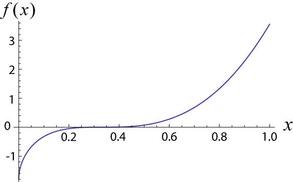
f⁡(x)≡8​3​x5/2−323​x3/2+163​x+83​x1/2−169<0,\displaystyle f(x)\equiv 8\sqrt{3}x^{5/2}-\frac{32}{\sqrt{3}}x^{3/2}+\frac{16}{3}x+\frac{8}{\sqrt{3}}x^{1/2}-\frac{16}{9}<0, (38)

where x≡c~1/c~2x\equiv\tilde{c}_{1}/\tilde{c}_{2}. The function f⁡(x)f(x) on the left-hand side of Eq. (38) is plotted in Fig. 6, from which we find that the UN state becomes dynamically unstable and the system is driven towards the BN phase if x<1/3x<1/3, or equivalently, if c1<0c_{1}<0. Since the UN-BN phase boundary is at c1=0c_{1}=0, there is no parameter regime in which the UN state is metastable. However, it should be noted that for c1<0c_{1}<0, where the BN phase is the ground state, the UN state becomes dynamically unstable and cannot exist as an excited state since the excitation modes would grow exponentially. In other words, there is no level crossing in the UN-BN phase transition in contrast to the ferromagnetic-cyclic one. It should be stressed that this result, which was derived from the stability analysis, is stronger than the result obtained in Refs. [30, 31] since it implies not only that the UN phase is no longer the ground state for c1<0c_{1}<0 but also that it is not even an excited state due to the dynamical instability.
Refer to caption
Figure 6: Plot of f⁡(x)f(x) defined in Eq. (38)

IV Symmetry-prohibited metastability

In the previous section, the stability analysis based on the Beliaev theory states that the ferromagnetic-cyclic and UN-BN phase transitions are not accompanied by metastable states. In this section, we show that the absence of metastability holds to all orders of approximation since the metastability is prohibited by the high symmetry of the Hamiltonian at the phase boundary. We investigate the underlying symmetry of the Hamiltonian that results in a flat energy landscape at the phase boundary in both spin-1 and spin-2 BECs. This energy landscape prohibits a coexistence of two phases as opposed to the double-well structure in conventional first-order phase transitions.

IV.1 Spin-1 BECs

In the presence of a quadratic Zeeman effect, the interaction Hamiltonian of a spin-1 BEC is given by

V^=∫d𝐫(c02:n^2:+c12:𝐅^2:+q∑j=−11j2ψ^j†ψ^j),\displaystyle\hat{V}=\int\text{d}\mathbf{r}\,\left(\frac{c_{0}}{2}:\hat{n}^{2}:+\frac{c_{1}}{2}:\hat{\mathbf{F}}^{2}:+q\sum_{j=-1}^{1}j^{2}\hat{\psi}_{j}^{\dagger}\hat{\psi}_{j}\right), (39)

where qq denotes the quadratic Zeeman coefficient, and n^\hat{n} and F^\hat{F} are the number density and spin density operators. The linear Zeeman energy is suppressed due to the conservation of the total spin of an isolated system. The mean-field ground-state phase diagrams of spin-1 BECs are shown in Fig. 7 for the cases of Rb87{}^{\text{87}}\text{Rb} and Na23{}^{\text{23}}\text{Na} (see, for example, Ref. [14]). The order parameter of the ferromagnetic, antiferromagnetic, and polar phases are 𝝃FM=(1,0,0)T\bm{\xi}^{\mathrm{FM}}=(1,0,0)^{\mathrm{T}}, 𝝃AFM=(1,0,1)T/2\bm{\xi}^{\mathrm{AFM}}=(1,0,1)^{\mathrm{T}}/\sqrt{2}, and 𝝃PL=(0,1,0)T\bm{\xi}^{\mathrm{PL}}=(0,1,0)^{\mathrm{T}}, respectively, while the order parameter of the broken-axisymmetry (BA) phase varies continuously as a function of qq from 𝝃BA=(1,2,1)T/2\bm{\xi}^{\mathrm{BA}}=(1,\sqrt{2},1)^{\mathrm{T}}/2 at q=0q=0 to 𝝃BA=(0,1,0)T\bm{\xi}^{\mathrm{BA}}=(0,1,0)^{\mathrm{T}} at q=2​|c1|​nq=2|c_{1}|n. From the discontinuity in the transformation of the order parameter at the phase boundary, it is clear that the ferromagnetic-BA and antiferromagnetic-polar phase transitions are first order, while the BA-polar phase transition is second order. This is also confirmed by examining the discontinuity in the first derivative of the ground-state energy with respect to the quadratic Zeeman shift qq that drives these transitions (see Appendix B). We now show that these first-order quantum phase transitions are not accompanied by metastable states, and this holds to all orders of approximation. At nonzero qq, the Hamiltonian has the U(1)ϕ×{}_{\phi}\timesSO(2)fz{}_{f_{z}} symmetry involving gauge and rotational invariants along the zz axis in spin space. Only at q=0q=0 does the Hamiltonian possess a larger symmetry of U(1)ϕ×{}_{\phi}\timesSO(3)f, corresponding to a full rotational invariant in spin space. On the other hand, the order parameters of each pair of two phases in the above first-order phase transitions at q=0q=0 can be transformed between each other via an SO(3) rotation, 𝝃BA​(q=0)=ei​fy​π/2​𝝃FM,𝝃PL=ei​fy​π/2​𝝃AFM\bm{\xi}^{\mathrm{BA}}(q=0)=e^{if_{y}\pi/2}\bm{\xi}^{\mathrm{FM}},\bm{\xi}^{\mathrm{PL}}=e^{if_{y}\pi/2}\bm{\xi}^{\mathrm{AFM}}. Therefore, the two phases are degenerate at q=0q=0 to any order of approximation. Namely, the phase boundary at q=0q=0 remains unchanged even when quantum corrections are added to the ground-state energy. Furthermore, if we use a parameter θ\theta to represent the order parameters of the intermediate states in the transformation from the ferromagnetic (antiferromagnetic) to the BA (polar) phase: ei​fy​θ​𝝃FM=(cos2⁡(θ/2),sin⁡θ/2,sin2⁡(θ/2))Te^{if_{y}\theta}\bm{\xi}^{\mathrm{FM}}=(\cos^{2}(\theta/2),\sin\theta/\sqrt{2},\sin^{2}(\theta/2))^{\mathrm{T}} (ei​fy​θ​𝝃AFM=(sin⁡θ/2,cos⁡θ,sin⁡θ/2)Te^{if_{y}\theta}\bm{\xi}^{\mathrm{AFM}}=(\sin\theta/\sqrt{2},\cos\theta,\sin\theta/\sqrt{2})^{\mathrm{T}}) (0⩽θ⩽π/20\leqslant\theta\leqslant\pi/2), all these intermediate states are energy degenerate; i.e., E⁡(θ)E(\theta) is independent of θ\theta, resulting in a flat energy landscape at q=0q=0. As qq crosses the phase boundary from the negative to the positive side, the ferromagnetic and antiferromagnetic phases immediately change from the ground state (the global minimum in the energy landscape) to an unstable state (a local maximum in the energy landscape if existing), leading to no parameter regime of metastability. Similarly, no metastable regime exists for the BA and polar phases as qq crosses the phase boundary from the positive to the negative side. This can be understood by looking at the mean-field energy landscape

EFM−BA​(θ)/V=\displaystyle E^{\mathrm{FM-BA}}(\theta)/V= (c0+c1)​n22+q​n​(1−sin2⁡θ2),\displaystyle\frac{(c_{0}+c_{1})n^{2}}{2}+qn\left(1-\frac{\sin^{2}\theta}{2}\right), (40)
EAFM−PL​(θ)/V=\displaystyle E^{\mathrm{AFM-PL}}(\theta)/V= c0​n22+q​n​sin2⁡θ,\displaystyle\frac{c_{0}n^{2}}{2}+qn\sin^{2}\theta, (41)

where the maximum and minimum at θ=0\theta=0 and θ=π/2\theta=\pi/2, respectively, are exchanged as qq crosses zero. A comparison with the conventional first-order phase transitions whose energy landscapes feature a double well and thus support metastability is illustrated in Fig. 8. However, the absence of metastability holds not only at the mean-field level but also to all orders of approximation since the above argument of the flat energy landscape at the phase boundary is based on the symmetry of the Hamiltonian.

Refer to caption
Figure 7: (Color online) Mean-field ground-state phase diagrams of spin-1 (a) Rb87{}^{\text{87}}\text{Rb} and (b) Na23{}^{\text{23}}\text{Na} BECs where the spin-dependent interaction is ferromagnetic (c1<0c_{1}<0) and antiferromagnetic (c1>0c_{1}>0), respectively. The ground-state phase depends on the ratio of the quadratic Zeeman energy qq to the interaction energy |c1|​n|c_{1}|n. The inset in each phase shows the surface plot of |ψ⁡(θ,ϕ)|2≡|∑m=−11ξm​Y1m​(θ,ϕ)|2|\psi(\theta,\phi)|^{2}\equiv|\sum_{m=-1}^{1}\xi_{m}Y_{1}^{m}(\theta,\phi)|^{2}, where Y1mY_{1}^{m}’s are the spherical harmonic functions of rank 1. The order parameter 𝝃BA\bm{\xi}^{\mathrm{BA}} of the broken-axisymmetry (BA) phase varies continuously as a function of q/|c1|​nq/|c_{1}|n. The ferromagnetic-BA and antiferromagnetic-polar phase transitions are first order, while the BA-polar phase transition is second order.
Refer to caption
Figure 8: Energy landscape against the order parameter for first-order quantum phase transitions (a) with and (b) without metastability [see Eq. (41)]. The transition between A and B phases is controlled by a change in the parameter cc (interaction c1c_{1} or c2c_{2} in Fig. 1 or the quadratic Zeeman shift qq in Fig. ). Here, cA−Bc^{\mathrm{A-B}} indicates the phase boundary between the two phases, while cA−unstablec^{\mathrm{A-unstable}} represents the value of cc at which the A phase becomes absolutely unstable. The energy landscape in (a) features a double well at c=cA−Bc=c^{A-B}, supporting a metastable state around the transition point, whereas the energy landscape in (b) becomes flat at c=cA−Bc=c^{A-B}, allowing no metastable state.

IV.2 Spin-2 BECs

Now we show that the absence of metastability in the ferromagnetic-cyclic and UN-BN phase transitions, which was proved up to the second order by the stability analysis in Sec. III.3, holds to all orders of approximation due to the symmetry of the Hamiltonian. For finite c1c_{1}, the Hamiltonian of spin-2 BECs [Eq. (2)] has the U(1)ϕ×{}_{\phi}\timesSO(3)f symmetry. Only at c1=0c_{1}=0 is its symmetry enlarged to U(1)ϕ×{}_{\phi}\timesSO(5)f due to the invariance of the spin-singlet-pair interaction c2:A^00†​A^00:c_{2}:\hat{A}_{00}^{\dagger}\hat{A}_{00}: under a rotation in the Hilbert space composed of five magnetic sublevels [32]. On the other hand, from the order parameters 𝝃FM=(1,0,0,0,0)T\bm{\xi}^{\mathrm{FM}}=(1,0,0,0,0)^{\mathrm{T}} and 𝝃CL=(1,0,0,2,0)T/3\bm{\xi}^{\mathrm{CL}}=(1,0,0,\sqrt{2},0)^{\mathrm{T}}/\sqrt{3}, the ferromagnetic and cyclic phases both have zero spin-singlet-pair amplitude ⟨A^00⟩=0\langle\hat{A}_{00}\rangle=0. Similarly, the UN (𝝃UN=(0,0,1,0,0)T\bm{\xi}^{\mathrm{UN}}=(0,0,1,0,0)^{\mathrm{T}}) and BN (𝝃BN=(1,0,0,0,1/)T/2\bm{\xi}^{\mathrm{BN}}=(1,0,0,0,1/)^{\mathrm{T}}/\sqrt{2}) phases both have the maximum value of the spin-singlet-pair amplitude ⟨A^00⟩=1\langle\hat{A}_{00}\rangle=1. In other words, the ferromagnetic and cyclic phases (UN and BN phases) belong to the same group of the minimum (maximum) value of spin-singlet-pair amplitude whose elements can be transformed between each other by SO(5) rotations. Therefore, these pairs of phases are degenerate at c1=0c_{1}=0 where the Hamiltonian possesses the same symmetry. That the energy degeneracy holds to all orders of approximation makes the phase boundary at c1=0c_{1}=0 remain unchanged even when quantum corrections to the ground-state energy are taken into account. Furthermore, similar to the spin-1 BECs, if the order parameters of the intermediate states in the transformation from the ferromagnetic (UN) to the cyclic (BN) phase are parametrized as U⁡(η)​𝝃FM=(cos⁡η,0,0,sin⁡η,0)TU(\eta)\bm{\xi}^{\mathrm{FM}}=(\cos\eta,0,0,\sin\eta,0)^{\mathrm{T}} [U′​(η)​𝝃UN=(sin⁡η/2,0,cos⁡η,0,sin⁡η/2)TU^{\prime}(\eta)\bm{\xi}^{\mathrm{UN}}=(\sin\eta/\sqrt{2},0,\cos\eta,0,\sin\eta/\sqrt{2})^{\mathrm{T}}], where U⁡(η)U(\eta) [U′​(η)U^{\prime}(\eta)] is an SO(5) rotation operator, all these intermediate states are energy degenerate; i.e., E⁡(η)E(\eta) is independent of η\eta, resulting in a flat energy landscape at c1=0c_{1}=0 (see Fig. 9). As c1c_{1} crosses the phase boundary from the negative to the positive side, the ferromagnetic and BN phases abruptly changes from the ground state (the global minimum in the energy landscape) to an unstable state (a local maximum, if it exists), leading to no region of metastability. Similarly, no metastable regime exists for the cyclic and UN phases as c1c_{1} crosses the phase boundary from the positive to the negative side. This is illustrated by the energy landscape of the ground-state manifold of nematic phase [31, 32] [see Eq. (52)]

EUN−BN​(η)V=\displaystyle\frac{E^{\mathrm{UN-BN}}(\eta)}{V}=\, ω​∑j=02[1−2​c12​c1−c2/5​cos⁡(2​η+2​π​j3)]52\displaystyle\omega\sum_{j=0}^{2}\left[1-\frac{2c_{1}}{2c_{1}-c_{2}/5}\cos\left(2\eta+\frac{2\pi j}{3}\right)\right]^{\frac{5}{2}}
+η​-independent terms,\displaystyle+\eta\text{-independent terms}, (42)

where ω≡8​M3/2​[n⁡(2​c1−c2/5)]5/2/(15​π2​ℏ3)\omega\equiv 8M^{3/2}[n(2c_{1}-c_{2}/5)]^{5/2}/(15\pi^{2}\hbar^{3}). Equation (42) takes the minimum (maximum) value at η=n​π/3\eta=n\pi/3 (η=π/6+n​π/3\eta=\pi/6+n\pi/3) (n=0,1,…n=0,1,\dots) corresponding to the UN (BN) phase for c1>0c_{1}>0 and the maximum (minimum) value for c1<0c_{1}<0. It means that the UN phase changes abruptly from the ground state to an unstable state as the phase boundary is crossed at c1=0c_{1}=0, implying no parameter regime of metastable states. Since the above argument of the flat energy landscape is based on the symmetry of the Hamiltonian, the absence of metastability is valid to all orders of approximation.

Refer to caption
Figure 9: (Color online) SO(5) rotations connecting (a) UN and BN phases and (b) ferromagnetic and cyclic phases. The order parameters and the spherical harmonic representations of the initial, final, and intermediate states are displayed.

V Macroscopic Quantum Tunneling

The presence of a metastable state (Sec. III.3) implies an interesting possibility of a decay of the metastable state into the lower energy state via MQT; i.e., all atoms tunnel simultaneously from one phase to the other. We consider this possibility for the metastable state near the UN-cyclic phase boundary, as the parameters of the spin-2 Rb87{}^{\text{87}}\text{Rb} BEC are thought to lie near this phase boundary [35]. Equation (32) shows that there is a parameter regime in which the UN phase is metastable, and the cyclic phase is the ground state. By neglecting quantum depletion, these states are described by

|UN⟩≃\displaystyle|\mathrm{UN}\rangle\simeq (a^0†)N​|vac⟩,\displaystyle\left(\hat{a}_{0}^{\dagger}\right)^{N}|\mathrm{vac}\rangle, (43a)
|Cyclic⟩≃\displaystyle|\mathrm{Cyclic}\rangle\simeq (a^2†2+a^0†2+a^−2†2)N​|vac⟩,\displaystyle\left(\frac{\hat{a}_{2}^{\dagger}}{2}+\frac{\hat{a}_{0}^{\dagger}}{\sqrt{2}}+\frac{\hat{a}_{-2}^{\dagger}}{2}\right)^{N}|\mathrm{vac}\rangle, (43b)

where a^m†\hat{a}_{m}^{\dagger} is the creation operator of a particle with zero momentum and magnetic quantum number mF=mm_{F}=m. Since these states are not the exact eigenstates of the many-body Hamiltonian (2), they will undergo quantum diffusions in spin space [44, 45, 46, 47] and induce MQT. We now estimate the time scale of MQT by restricting the Hilbert space to the two states at local energy minima. The time scale of MQT is then given by τ=ℏ/Δ\tau=\hbar/\Delta with Δ=2​⟨Cyclic|V^|UN⟩\Delta=2\langle\mathrm{Cyclic}|\hat{V}|\mathrm{UN}\rangle. Using Eqs. (43) and (2), we obtain

τ≃ℏ​2N/2c0​n​(N−1),\displaystyle\tau\simeq\hbar\frac{2^{N/2}}{c_{0}n(N-1)}, (44)

where NN is the total number of particles. The exponentially large factor of 2N/22^{N/2} reflects macroscopic magnification in a BEC. To observe MQT, τ\tau must be equal to or smaller than the lifetime of the BEC, which is of the order of a second. Substituting parameters of Rb87{}^{\text{87}}\text{Rb} into Eq. (44), we can estimate an upper bound for the total number of particles: Nmax≃36N_{\mathrm{max}}\simeq 36 for τ≲1\tau\lesssim 1 s. A similar time scale is expected for MQT across the ferromagnetic-BN transition.

VI Conclusion

We have shown that spinor BECs exhibit two distinct types of first-order quantum phase transitions: one in which metastable states are induced by quantum fluctuations and the other in which the metastability is prohibited by the symmetry of the Hamiltonian at the phase boundary. By developing the spinor Beliaev theory which takes account of the effect of quantum fluctuations, the appearance of the metastability in the former that cannot be captured by the Bogoliubov theory has been revealed. In contrast, for the latter, the absence of metastability has been deduced from a general argument of the energy landscape which becomes flat at the phase boundary. The absence of metastability holds to all orders of approximation due to the symmetry of the Hamiltonian. Some of these first-order phase transitions in spin-1 and spin-2 BECs are within reach of current experiments. The present study has shed light on the pivotal role of quantum fluctuations in the first-order quantum phase transitions. With the importance of the effect of quantum fluctuations shown above, it is worth investigating the implication of this study to closely related problems such as the Coleman-Weinberg mechanism of quantum symmetry breaking [48], quantum anomaly [49], and quasi-Nambu-Goldstone modes [50]. It would also be of interest to study the dynamics of the first-order quantum phase transitions without metastability since criticality might arise from the flat energy landscape at the phase boundary.

Acknowledgements.
This work was supported by KAKENHI Grant No. 22340114 from the Japan Society for the Promotion of Science, and a Grant-in-Aid for Scientific Research on Innovation Areas “Topological Quantum Phenomena” (KAKENHI Grant No. 22103005), and the Photon Frontier Network Program from MEXT of Japan. Y.K. acknowledges the financial support from KAKENHI Grant No.22740265, FIRST, and Inoue Foundation.

Appendix A Ground-state energies with the LHY corrections

For a dilute homogeneous system of spinless bosons, the ground-state energy density up to the LHY correction is given by [19, 20]

EV=2​π​ℏ2​a​n2M​(1+12815​π​n​a3),\displaystyle\frac{E}{V}=\frac{2\pi\hbar^{2}an^{2}}{M}\left(1+\frac{128}{15\sqrt{\pi}}\sqrt{na^{3}}\right), (45)

where nn, aa, and MM are the particle-number density, the ss-wave scattering length, and the atomic mass, respectively. The first term on the right-hand side of Eq. (45) is the Hartree mean-field energy, while the second term gives the leading-order correction first derived by Lee, Huang, and Yang [19, 20]. The LHY correction arises from virtual excitations (i.e., quantum fluctuations) of the condensate and is proportional to the fraction of quantum depletion: nqd/n=8​n​a3/(3​π)n^{\mathrm{qd}}/n=8\sqrt{na^{3}}/(3\sqrt{\pi}). In the following, we calculate the ground-state energies of the four possible phases of spin-2 BECs, from which the beyond-mean-field phase boundaries in Fig. 1 are determined.

Ferromagnetic and BN phases.–With the LHY corrections for spinor Bose gases, the ground-state energy densities of the ferromagnetic and BN phases for c1<0c_{1}<0 and c2≃20​c1c_{2}\simeq 20c_{1} are given by [32]

EFMV=\displaystyle\frac{E^{\mathrm{FM}}}{V}= (c02+2​c1)​n2​[1+16​M3/215​π2​ℏ3​n​(c0+4​c1)3]\displaystyle\,\left(\frac{c_{0}}{2}+2c_{1}\right)n^{2}\left[1+\frac{16M^{3/2}}{15\pi^{2}\hbar^{3}}\sqrt{n(c_{0}+4c_{1})^{3}}\right] (46)

and

EBNV=\displaystyle\frac{E^{\mathrm{BN}}}{V}= (c02+c210)​n2​[1+16​M3/215​π2​ℏ3​n​(c0+4​c1)3]\displaystyle\,\left(\frac{c_{0}}{2}+\frac{c_{2}}{10}\right)n^{2}\left[1+\frac{16M^{3/2}}{15\pi^{2}\hbar^{3}}\sqrt{n\left(c_{0}+4c_{1}\right)^{3}}\right]
+8​M3/215​π2​ℏ3​(32+18​3)​(|c1|​n)5/2\displaystyle+\frac{8M^{3/2}}{15\pi^{2}\hbar^{3}}(32+18\sqrt{3})(|c_{1}|n)^{5/2}
+𝒪⁡[M3/2​n5/2​max​{c03/2,|c1|3/2}​|c2−20​c1|ℏ3],\displaystyle+\mathcal{O}\left[\frac{M^{3/2}n^{5/2}\mathrm{max}\left\{c_{0}^{3/2},|c_{1}|^{3/2}\right\}|c_{2}-20c_{1}|}{\hbar^{3}}\right], (47)

respectively. By noting that |c2−20​c1|∼M3/2​n1/2​|c1|5/2/ℏ3|c_{2}-20c_{1}|\sim M^{3/2}n^{1/2}|c_{1}|^{5/2}/\hbar^{3} near the phase boundary [see Eq. (3)], the last term in Eq. (47) is smaller than the other terms by a factor of n​a3≪1\sqrt{na^{3}}\ll 1 with a≡(4​a2+3​a4)/7=c0​M/(4​π​ℏ2)a\equiv(4a_{2}+3a_{4})/7=c_{0}M/(4\pi\hbar^{2}) and thus is negligible. Consequently, the boundary between the ferromagnetic and BN phases is shifted from its Hartree mean-field boundary at c2=20​c1c_{2}=20c_{1} to

c2FM−BN≃\displaystyle c_{2}^{\mathrm{FM-BN}}\simeq  20​c1−32​(16+9​3)​M3/2​n1/2​|c1|5/23​π2​ℏ3\displaystyle\,20c_{1}-\frac{32(16+9\sqrt{3})M^{3/2}n^{1/2}|c_{1}|^{5/2}}{3\pi^{2}\hbar^{3}}
≃\displaystyle\simeq  20​c1−1521​(|c1|c0)3/2​n​a3​|c1|.\displaystyle\,20c_{1}-1521\left(\frac{|c_{1}|}{c_{0}}\right)^{3/2}\sqrt{na^{3}}\,|c_{1}|. (48)

Thus, we have derived Eq. (3).

Cyclic and UN phases.–Similarly, the ground-state energy densities of the cyclic and UN phases with the LHY corrections for c1>0c_{1}>0 and c2≤0c_{2}\leq 0 are respectively given by [32]

ECLV=\displaystyle\frac{E^{\mathrm{CL}}}{V}= c0​n22+8​M3/215​π2​ℏ3​[(n​c0)5/2+12​2​(n​c1)5/2]\displaystyle\,\frac{c_{0}n^{2}}{2}+\frac{8M^{3/2}}{15\pi^{2}\hbar^{3}}\left[(nc_{0})^{5/2}+12\sqrt{2}(nc_{1})^{5/2}\right] (49)

and

EUNV=\displaystyle\frac{E^{\mathrm{UN}}}{V}= (c0+c25)​n22\displaystyle\,\left(c_{0}+\frac{c_{2}}{5}\right)\frac{n^{2}}{2}
+8​M3/215​π2​ℏ3​[(n​c0)5/2+18​3​(n​c1)5/2]\displaystyle+\frac{8M^{3/2}}{15\pi^{2}\hbar^{3}}\Big[(nc_{0})^{5/2}+18\sqrt{3}(nc_{1})^{5/2}\Big]
+𝒪⁡[M3/2​n5/2​max​{c03/2,c13/2}​|c2|ℏ3].\displaystyle+\mathcal{O}\left[\frac{M^{3/2}n^{5/2}\mathrm{max}\left\{c_{0}^{3/2},c_{1}^{3/2}\right\}|c_{2}|}{\hbar^{3}}\right]. (50)

Here, EUNE^{\mathrm{UN}} is expanded in powers of c2/c0c_{2}/c_{0} and c2/c1c_{2}/c_{1}, which are expected to be small near the UN-cyclic phase boundary. In fact, since |c2|∼M3/2​n1/2​c15/2/ℏ3|c_{2}|\sim M^{3/2}n^{1/2}c_{1}^{5/2}/\hbar^{3} at the phase boundary [see Eq. (4)], the last term in Eq. (50) is smaller than the others by a factor of n​a3≪1\sqrt{na^{3}}\ll 1, and thus can be ignored. By comparing the energies in Eqs. (49) and (50), we find that the phase boundary between the UN and cyclic phases is given by

c2UN−CL≃\displaystyle c_{2}^{\mathrm{UN-CL}}\simeq −16​(18​3−12​2)​M3/2​n1/2​c15/23​π2​ℏ3\displaystyle\,-\frac{16(18\sqrt{3}-12\sqrt{2})M^{3/2}n^{1/2}c_{1}^{5/2}}{3\pi^{2}\hbar^{3}}
≃\displaystyle\simeq −342​(c1c0)3/2​n​a3​c1.\displaystyle\,-342\left(\frac{c_{1}}{c_{0}}\right)^{3/2}\sqrt{na^{3}}\,c_{1}. (51)

Thus, we have derived Eq. (4).

Appendix B Finite jump in the first derivative of energy

Thermal phase transitions are identified to be first order if there is a discontinuity in the first derivative of the free energy with respect to temperature. Similarly, a quantum phase transition is first order if there is a discontinuity in the first derivative of the ground-state energy with respect to the parameter that drives the transition. In the following, the first derivative of the energy will be calculated at each of the phase boundaries in Fig. 1. The ground-state energies of the ferromagnetic and cyclic phases are given by Eqs. (46) and (49), respectively, while those of the UN and BN phases are obtained from the expression for the energy of the manifold of nematic phase [31, 32]:

E⁡(η)V=\displaystyle\frac{E(\eta)}{V}= (c0+c25)​n22​[1+16​M3/2​n1/215​π2​ℏ3​(c0+c25)3/2]\displaystyle\,\left(c_{0}+\frac{c_{2}}{5}\right)\frac{n^{2}}{2}\left[1+\frac{16M^{3/2}n^{1/2}}{15\pi^{2}\hbar^{3}}\left(c_{0}+\frac{c_{2}}{5}\right)^{3/2}\right]
+8​M3/2​n5/215​π2​ℏ3{(|c2|5)5/2+(2c1−c25)5/2\displaystyle+\frac{8M^{3/2}n^{5/2}}{15\pi^{2}\hbar^{3}}\Bigg\{\left(\frac{|c_{2}|}{5}\right)^{5/2}+\left(2c_{1}-\frac{c_{2}}{5}\right)^{5/2}
×∑j=02[1−2​c12​c1−c2/5cos(2η+2​π​j3)5/2]},\displaystyle\times\sum\limits_{j=0}^{2}\left[1-\frac{2c_{1}}{2c_{1}-c_{2}/5}\cos\left(2\eta+\frac{2\pi j}{3}\right)^{5/2}\right]\Bigg\}, (52)

where η=n​π/3\eta=n\pi/3 (η=π/6+n​π/3\eta=\pi/6+n\pi/3) corresponds to the UN (BN) phase.

Ferromagnetic-BN phase transition.–We have

∂(EFM/V)∂c2=\displaystyle\frac{\partial(E^{\mathrm{FM}}/V)}{\partial c_{2}}= 0,\displaystyle 0, (53a)
∂(EBN/V)∂c2|c2=c2FM−BN=\displaystyle\frac{\partial(E^{\mathrm{BN}}/V)}{\partial c_{2}}\Big|_{c_{2}=c_{2}^{\mathrm{FM-BN}}}= n210​[1+𝒪​(n​a3)],\displaystyle\frac{n^{2}}{10}\left[1+\mathcal{O}(\sqrt{na^{3}})\right], (53b)

where c2FM−BNc_{2}^{\mathrm{FM-BN}} is given by Eq. (3). Equation (53) implies that there is a jump in ∂E/∂c2\partial E/\partial c_{2} at the phase boundary of the ferromagnetic-BN transition. Therefore, it can be identified as the first-order phase transition.

UN-cyclic phase transition.–Similarly, the first derivatives of the ground-state energies at the phase boundary c2UN−CLc_{2}^{\mathrm{UN-CL}} given by Eq. (4) are

∂(ECL/V)∂c2=\displaystyle\frac{\partial(E^{\mathrm{CL}}/V)}{\partial c_{2}}= 0,\displaystyle 0, (54)
∂(EUN/V)∂c2|c2=c2UN−CL=\displaystyle\frac{\partial(E^{\mathrm{UN}}/V)}{\partial c_{2}}\Big|_{c_{2}=c_{2}^{\mathrm{UN-CL}}}= n210​[1+𝒪​(n​a3)].\displaystyle\frac{n^{2}}{10}\left[1+\mathcal{O}(\sqrt{na^{3}})\right]. (55)

Therefore, the cyclic-UN phase transition is first order.

Ferromagnetic-cyclic phase transition.–The first derivatives of the energies with respect to c1c_{1} at the phase boundary c1=0,c2>0c_{1}=0,c_{2}>0 are obtained as

∂(EFM/V)∂c1|c1=0=\displaystyle\frac{\partial(E^{\mathrm{FM}}/V)}{\partial c_{1}}\Big|_{c_{1}=0}= n2​[2+𝒪​(n​a3)],\displaystyle n^{2}\left[2+\mathcal{O}(\sqrt{na^{3}})\right], (56)
∂(ECL/V)∂c1|c1=0=\displaystyle\frac{\partial(E^{\mathrm{CL}}/V)}{\partial c_{1}}\Big|_{c_{1}=0}= 0.\displaystyle 0. (57)

This implies that the ferromagnetic-cyclic phase transition is first order.

UN-BN phase transition.–The first derivatives of the energies with respect to c1c_{1} at the phase boundary c1=0,c2<0c_{1}=0,c_{2}<0 up to the level of the LHY correction are given by

∂(EUN/V)∂c1|c1=0=\displaystyle\frac{\partial(E^{\mathrm{UN}}/V)}{\partial c_{1}}\Big|_{c_{1}=0}= 8​M3/2​n5/2​|c2|3/2π2​ℏ3,\displaystyle\frac{8M^{3/2}n^{5/2}|c_{2}|^{3/2}}{\pi^{2}\hbar^{3}}, (58)
∂(EBN/V)∂c1|c1=0=\displaystyle\frac{\partial(E^{\mathrm{BN}}/V)}{\partial c_{1}}\Big|_{c_{1}=0}= 8​M3/2​n5/2​|c2|3/2π2​ℏ3.\displaystyle\frac{8M^{3/2}n^{5/2}|c_{2}|^{3/2}}{\pi^{2}\hbar^{3}}. (59)

Up to this order, the first derivative changes continuously. However, since there is a discontinuity in the transformation of the order parameters at the UN-BN phase boundary, the phase transition must be first order, and thus, it is expected that with higher-order corrections to the ground-state energy, a jump in ∂E/∂c1\partial E/\partial c_{1} should appear at c1=0c_{1}=0. The difference in the order of approximation at which a jump in the energy derivative appears between the UN-BN and the other phase transitions in spin-2 BECs is related to the fact that the UN-BN phase transition only appears for the first time as the zero-point-energy fluctuations is taken into account. This will be investigated in a future publication.

Similarly, the fact that the ferromagnetic-BA and antiferromagnetic-polar phase transitions in spin-1 BECs are first order can also be confirmed by a finite jump in the first derivative of the ground-state energy with respect to the quadratic Zeeman shift qq that drives these transitions [32, 14]. Both of these phase transitions occur at q=0q=0.

Ferromagnetic-BA phase transition. The first derivatives of the ground-state energy with respect to qq at the phase boundary are given for the two phases as follows.

∂(EFM/V)∂q|q=0=\displaystyle\frac{\partial(E^{\mathrm{FM}}/V)}{\partial q}\Big|_{q=0}= n,\displaystyle n, (60)
∂(EBA/V)∂q|q=0=\displaystyle\frac{\partial(E^{\mathrm{BA}}/V)}{\partial q}\Big|_{q=0}= n2​[1+𝒪​(n​a3)].\displaystyle\frac{n}{2}\left[1+\mathcal{O}(\sqrt{na^{3}})\right]. (61)

Antiferromagnetic-polar phase transition. Similarly, we have

∂(EAFM/V)∂q|q=0=\displaystyle\frac{\partial(E^{\mathrm{AFM}}/V)}{\partial q}\Big|_{q=0}= n⁡[1+𝒪⁡(n​a3)],\displaystyle n\left[1+\mathcal{O}(\sqrt{na^{3}})\right], (62)
∂(EPL/V)∂q|q=0=\displaystyle\frac{\partial(E^{\mathrm{PL}}/V)}{\partial q}\Big|_{q=0}= 0+𝒪⁡(n​a3).\displaystyle 0+\mathcal{O}(\sqrt{na^{3}}). (63)

Appendix C Bogoliubov excitation spectra

The Bogoliubov excitation spectra of the four phases of spin-2 BECs in Fig. 1 at zero magnetic field and the associated possible instabilities are listed as follows [32, 14]. For spin-2 BECs, there are five excitation modes for each phase.

Ferromagnetic phase. The excitation spectra are given by

ϵ𝐩0​[ϵ𝐩0+2​(c0+4​c1)​n],\displaystyle\sqrt{\epsilon^{0}_{\mathbf{p}}\left[\epsilon^{0}_{\mathbf{p}}+2(c_{0}+4c_{1})n\right]}, (64)
ϵ𝐩0,\displaystyle\epsilon^{0}_{\mathbf{p}}, (65)
ϵ𝐩0−4​c1​n,\displaystyle\epsilon^{0}_{\mathbf{p}}-4c_{1}n, (66)
ϵ𝐩0−6​c1​n,\displaystyle\epsilon^{0}_{\mathbf{p}}-6c_{1}n, (67)
ϵ𝐩0−(8​c1−2​c2/5)​n.\displaystyle\epsilon^{0}_{\mathbf{p}}-(8c_{1}-2c_{2}/5)n. (68)

From Eq. (68), a Landau instability with a negative excitation energy would occur if c2<20​c1c_{2}<20c_{1}. Note that c1<0,c2=20​c1c_{1}<0,c_{2}=20c_{1} is the Hartree mean-field phase boundary of the ferromagnetic-BN phase transition, which is indicated by a dashed line in Fig. 1 [26].

Cyclic phase. The excitation spectra are given by

ϵ𝐩0​(ϵ𝐩0+2​c0​n),\displaystyle\sqrt{\epsilon^{0}_{\mathbf{p}}\left(\epsilon^{0}_{\mathbf{p}}+2c_{0}n\right)}, (69)
ϵ𝐩0​(ϵ𝐩0+4​c1​n),\displaystyle\sqrt{\epsilon^{0}_{\mathbf{p}}\left(\epsilon^{0}_{\mathbf{p}}+4c_{1}n\right)}, (70)
ϵ𝐩0+2​c2​n/5,\displaystyle\epsilon^{0}_{\mathbf{p}}+2c_{2}n/5, (71)
ϵ𝐩0​(ϵ𝐩0+4​c1​n),\displaystyle\sqrt{\epsilon^{0}_{\mathbf{p}}\left(\epsilon^{0}_{\mathbf{p}}+4c_{1}n\right)}, (72)
ϵ𝐩0​(ϵ𝐩0+4​c1​n).\displaystyle\sqrt{\epsilon^{0}_{\mathbf{p}}\left(\epsilon^{0}_{\mathbf{p}}+4c_{1}n\right)}. (73)

From Eq. (71), a Landau instability would occur if c2<0c_{2}<0. Note that c1>0,c2=0c_{1}>0,c_{2}=0 is the Hartree mean-field phase boundary of the UN-cyclic phase transition (dashed line in Fig. 1) [26].

UN phase. The excitation spectra are given by

ϵ𝐩0​[ϵ𝐩0+2​(c0+c2/5)​n],\displaystyle\sqrt{\epsilon^{0}_{\mathbf{p}}\left[\epsilon^{0}_{\mathbf{p}}+2(c_{0}+c_{2}/5)n\right]}, (74)
ϵ𝐩0​[ϵ𝐩0+2​(3​c1−c2/5)​n],\displaystyle\sqrt{\epsilon^{0}_{\mathbf{p}}\left[\epsilon^{0}_{\mathbf{p}}+2(3c_{1}-c_{2}/5)n\right]}, (75)
ϵ𝐩0​[ϵ𝐩0+2​(3​c1−c2/5)​n],\displaystyle\sqrt{\epsilon^{0}_{\mathbf{p}}\left[\epsilon^{0}_{\mathbf{p}}+2(3c_{1}-c_{2}/5)n\right]}, (76)
ϵ𝐩0​(ϵ𝐩0−2​c2​n/5),\displaystyle\sqrt{\epsilon^{0}_{\mathbf{p}}\left(\epsilon^{0}_{\mathbf{p}}-2c_{2}n/5\right)}, (77)
ϵ𝐩0​(ϵ𝐩0−2​c2​n/5).\displaystyle\sqrt{\epsilon^{0}_{\mathbf{p}}\left(\epsilon^{0}_{\mathbf{p}}-2c_{2}n/5\right)}. (78)

From Eq. (77), a dynamical instability, whose excitation energy involves a nonzero imaginary part, would occur if c2>0c_{2}>0.

BN phase. The excitation spectra are given by

ϵ𝐩0​[ϵ𝐩0+2​(c0+c2/5)​n],\displaystyle\sqrt{\epsilon^{0}_{\mathbf{p}}\left[\epsilon^{0}_{\mathbf{p}}+2(c_{0}+c_{2}/5)n\right]}, (79)
ϵ𝐩0​[ϵ𝐩0+2​(4​c1−c2/5)​n],\displaystyle\sqrt{\epsilon^{0}_{\mathbf{p}}\left[\epsilon^{0}_{\mathbf{p}}+2(4c_{1}-c_{2}/5)n\right]}, (80)
ϵ𝐩0​[ϵ𝐩0+2​(c1−c2/5)​n],\displaystyle\sqrt{\epsilon^{0}_{\mathbf{p}}\left[\epsilon^{0}_{\mathbf{p}}+2(c_{1}-c_{2}/5)n\right]}, (81)
ϵ𝐩0​[ϵ𝐩0+2​(c1−c2/5)​n],\displaystyle\sqrt{\epsilon^{0}_{\mathbf{p}}\left[\epsilon^{0}_{\mathbf{p}}+2(c_{1}-c_{2}/5)n\right]}, (82)
ϵ𝐩0​(ϵ𝐩0−2​c2​n/5).\displaystyle\sqrt{\epsilon^{0}_{\mathbf{p}}\left(\epsilon^{0}_{\mathbf{p}}-2c_{2}n/5\right)}. (83)

From Eq. (80), a dynamical instability would occur if c2>20​c1c_{2}>20c_{1}.

Appendix D Second-order self-energies

In this Appendix, we show the derivations of the contributions to the self-energies from the second-order Feynman diagrams that are used in Sec. III.3.

Ferromagnetic-BN phase transition.–The instability in the mF=−2m_{F}=-2 excitation mode of the ferromagnetic state causes the phase transition. Therefore, we calculate the self-energy Σ−2,−211​(2)\Sigma^{11(2)}_{-2,-2} and the chemical potential μ(2)\mu^{(2)} of the ferromagnetic state. The contribution to Σ−2,−211\Sigma^{11}_{-2,-2} from each of the second-order Feynman diagrams in Fig. 3 can be calculated straightforwardly in a manner similar to our previous work on spin-1 BECs [17]. By summing all these contributions, we obtain

ℏ​Σ−2,−211​(2)​(ω𝐩,𝐩)=\displaystyle\hbar\Sigma^{11(2)}_{-2,-2}(\omega_{\mathbf{p}},\mathbf{p})= [(c0−4​c1)2+4​c2225+4​c0​c25−16​c1​c25]​n0​∫d3​𝐪(2​π)3​(A2,𝐤+B2,𝐤−2​C2,𝐤ℏ​(ω𝐩−ω−2,𝐪(1)−ω2,𝐤(1))+i​η−𝒫​1ϵ𝐩0−ϵ𝐪0−ϵ𝐤0+i​η)\displaystyle\left[(c_{0}-4c_{1})^{2}+\frac{4c_{2}^{2}}{25}+\frac{4c_{0}c_{2}}{5}-\frac{16c_{1}c_{2}}{5}\right]n_{0}\int\frac{\text{d}^{3}\mathbf{q}}{(2\pi)^{3}}\,\left(\frac{A_{2,\mathbf{k}}+B_{2,\mathbf{k}}-2C_{2,\mathbf{k}}}{\hbar\left(\omega_{\mathbf{p}}-\omega^{(1)}_{-2,\mathbf{q}}-\omega^{(1)}_{2,\mathbf{k}}\right)+i\eta}-\mathcal{P}\frac{1}{\epsilon^{0}_{\mathbf{p}}-\epsilon^{0}_{\mathbf{q}}-\epsilon^{0}_{\mathbf{k}}+i\eta}\right)
+4(c1−c25)2n0∫d3​𝐪(2​π)3(1ℏ​(ω𝐩−ω−1,𝐪(1)−ω1,𝐤(1))+i​η−𝒫1ϵ𝐩0−ϵ𝐪0−ϵ𝐤0+i​η)\displaystyle+4\left(c_{1}-\frac{c_{2}}{5}\right)^{2}n_{0}\int\frac{\text{d}^{3}\mathbf{q}}{(2\pi)^{3}}\,\left(\frac{1}{\hbar\left(\omega_{\mathbf{p}}-\omega^{(1)}_{-1,\mathbf{q}}-\omega^{(1)}_{1,\mathbf{k}}\right)+i\eta}-\mathcal{P}\frac{1}{\epsilon^{0}_{\mathbf{p}}-\epsilon^{0}_{\mathbf{q}}-\epsilon^{0}_{\mathbf{k}}+i\eta}\right)
+2​c22​n025∫d3​𝐪(2​π)3(1ℏ​(ω𝐩−ω0,𝐪(1)−ω0,𝐤(1))+i​η−𝒫1ϵ𝐩0−ϵ𝐪0−ϵ𝐤0+i​η)\displaystyle+\frac{2c_{2}^{2}n_{0}}{25}\int\frac{\text{d}^{3}\mathbf{q}}{(2\pi)^{3}}\,\left(\frac{1}{\hbar\left(\omega_{\mathbf{p}}-\omega^{(1)}_{0,\mathbf{q}}-\omega^{(1)}_{0,\mathbf{k}}\right)+i\eta}-\mathcal{P}\frac{1}{\epsilon^{0}_{\mathbf{p}}-\epsilon^{0}_{\mathbf{q}}-\epsilon^{0}_{\mathbf{k}}+i\eta}\right)
+(c0−4c1+2​c25)∫d3​𝐪(2​π)3B2,𝐪,\displaystyle+\left(c_{0}-4c_{1}+\frac{2c_{2}}{5}\right)\int\frac{\text{d}^{3}\mathbf{q}}{(2\pi)^{3}}\,B_{2,\mathbf{q}}, (84)

where 𝐤≡𝐪−𝐩\mathbf{k}\equiv\mathbf{q}-\mathbf{p} and 𝒫\mathcal{P} denotes the principal value of the integral. Here, the first-order, i.e., the Bogoliubov, excitation spectra of the ferromagnetic phase are given by

ℏ​ω2,𝐩(1)=\displaystyle\hbar\omega^{(1)}_{2,\mathbf{p}}= ϵ𝐩0​[ϵ𝐩0+2​(c0+4​c1)​n0],\displaystyle\sqrt{\epsilon^{0}_{\mathbf{p}}[\epsilon^{0}_{\mathbf{p}}+2(c_{0}+4c_{1})n_{0}]}, (85)
ℏ​ω1,𝐩(1)=\displaystyle\hbar\omega^{(1)}_{1,\mathbf{p}}= ϵ𝐩0,\displaystyle\epsilon^{0}_{\mathbf{p}}, (86)
ℏ​ω0,𝐩(1)=\displaystyle\hbar\omega^{(1)}_{0,\mathbf{p}}= ϵ𝐩0−4​c1​n0,\displaystyle\epsilon^{0}_{\mathbf{p}}-4c_{1}n_{0}, (87)
ℏ​ω−1,𝐩(1)=\displaystyle\hbar\omega^{(1)}_{-1,\mathbf{p}}= ϵ𝐩0−6​c1​n0,\displaystyle\epsilon^{0}_{\mathbf{p}}-6c_{1}n_{0}, (88)
ℏ​ω−2,𝐩(1)=\displaystyle\hbar\omega^{(1)}_{-2,\mathbf{p}}= ϵ𝐩0−8​c1​n0+2​c2​n05,\displaystyle\epsilon^{0}_{\mathbf{p}}-8c_{1}n_{0}+\frac{2c_{2}n_{0}}{5}, (89)

and

A2,𝐤≡\displaystyle A_{2,\mathbf{k}}\equiv ℏ​ω2,𝐤(1)+ϵ𝐤0+(c0+4​c1)​n02​ℏ​ω2,𝐤(1),\displaystyle\frac{\hbar\omega^{(1)}_{2,\mathbf{k}}+\epsilon^{0}_{\mathbf{k}}+(c_{0}+4c_{1})n_{0}}{2\hbar\omega^{(1)}_{2,\mathbf{k}}}, (90)
B2,𝐤≡\displaystyle B_{2,\mathbf{k}}\equiv −ℏ​ω2,𝐤(1)+ϵ𝐤0+(c0+4​c1)​n02​ℏ​ω2,𝐤(1),\displaystyle\frac{-\hbar\omega^{(1)}_{2,\mathbf{k}}+\epsilon^{0}_{\mathbf{k}}+(c_{0}+4c_{1})n_{0}}{2\hbar\omega^{(1)}_{2,\mathbf{k}}}, (91)
C2,𝐤≡\displaystyle C_{2,\mathbf{k}}\equiv (c0+4​c1)​n02​ℏ​ω2,𝐤(1).\displaystyle\frac{(c_{0}+4c_{1})n_{0}}{2\hbar\omega^{(1)}_{2,\mathbf{k}}}. (92)

In order to find the zero-momentum excitation energy, we take 𝐩=𝟎\mathbf{p}=\bm{0}. Moreover, since it is expected that |ω−2,𝐩=𝟎−ω−2,𝐩=𝟎(1)|≪|c1|​n,|c2|​n|\omega_{-2,\mathbf{p}=\bm{0}}-\omega^{(1)}_{-2,\mathbf{p}=\bm{0}}|\ll|c_{1}|n,|c_{2}|n, which is justified by Eq. (19), we can replace the argument ω−2,𝐩=𝟎\omega_{-2,\mathbf{p}=\bm{0}} in Σ−2,−211​(2)\Sigma^{11(2)}_{-2,-2} by ω−2,𝐩=𝟎(1)\omega^{(1)}_{-2,\mathbf{p}=\bm{0}}. Equation (84) then can be evaluated straightforwardly, and we obtain

ℏ​Σ−2,−211​(2)=\displaystyle\hbar\Sigma^{11(2)}_{-2,-2}= (M​n0)3/2ℏ3{4​(c0+4​c1)1/23​π2[(c0−4c1)2+4​c2225+4​c0​c25−16​c1​c25]+2π(c1−c25)5/2+12​π(−c25)5/2\displaystyle\frac{(Mn_{0})^{3/2}}{\hbar^{3}}\Bigg\{\frac{4(c_{0}+4c_{1})^{1/2}}{3\pi^{2}}\left[(c_{0}-4c_{1})^{2}+\frac{4c_{2}^{2}}{25}+\frac{4c_{0}c_{2}}{5}-\frac{16c_{1}c_{2}}{5}\right]+\frac{\sqrt{2}}{\pi}\left(c_{1}-\frac{c_{2}}{5}\right)^{5/2}+\frac{1}{\sqrt{2}\pi}\left(\frac{-c_{2}}{5}\right)^{5/2}
+13​π2(c0+4c1)3/2(c0−4c1+2​c25)}.\displaystyle+\frac{1}{3\pi^{2}}(c_{0}+4c_{1})^{3/2}\left(c_{0}-4c_{1}+\frac{2c_{2}}{5}\right)\Bigg\}. (93)

Similarly, the total contribution to the chemical potential μ\mu from the second-order Feynman diagrams is calculated to be

μ(2)=\displaystyle\mu^{(2)}= 2​(c0+4​c1)​∫d3​𝐪(2​π)3​B2,𝐪+(c0+4​c1)​∫d3​𝐪(2​π)3​(−C2,𝐪+(c0+4​c1)​n02​ϵ𝐪0)\displaystyle 2(c_{0}+4c_{1})\int\frac{\text{d}^{3}\mathbf{q}}{(2\pi)^{3}}\,B_{2,\mathbf{q}}+(c_{0}+4c_{1})\int\frac{\text{d}^{3}\mathbf{q}}{(2\pi)^{3}}\,\left(-C_{2,\mathbf{q}}+\frac{(c_{0}+4c_{1})n_{0}}{2\epsilon^{0}_{\mathbf{q}}}\right)
=\displaystyle= 5​(M​n0)3/2​(c0+4​c1)5/23​π2​ℏ3.\displaystyle\frac{5(Mn_{0})^{3/2}(c_{0}+4c_{1})^{5/2}}{3\pi^{2}\hbar^{3}}. (94)

Near the ferromagnetic-BN phase boundary where c1,c2<0c_{1},c_{2}<0 and c2≃20​c1c_{2}\simeq 20c_{1}, from Eqs. (93) and (94) we have

ℏ​Σ−2,−211​(2)−μ(2)=\displaystyle\hbar\Sigma^{11(2)}_{-2,-2}-\mu^{(2)}= (36​3+64)​|c1|5/2​(M​n0)3/22​2​π​ℏ3\displaystyle\frac{(36\sqrt{3}+64)|c_{1}|^{5/2}(Mn_{0})^{3/2}}{2\sqrt{2}\pi\hbar^{3}}
+𝒪⁡(|c1|5/2​(M​n0)3/2​n​a3/ℏ3).\displaystyle+\mathcal{O}\left(|c_{1}|^{5/2}(Mn_{0})^{3/2}\sqrt{na^{3}}/\hbar^{3}\right). (95)

Here, we use n​a3≪1na^{3}\ll 1 with a≡c0​M/(4​π​ℏ2)a\equiv c_{0}M/(4\pi\hbar^{2}) so that the second term in Eq. (95) can be ignored. Thus, we have derived Eq. (18).

Ferromagnetic-cyclic phase transition.–The instability in the mF=−1m_{F}=-1 excitation mode of the ferromagnetic phase drives the phase transition. Therefore, we calculate Σ−1,−111​(2)\Sigma^{11(2)}_{-1,-1} of the ferromagnetic phase. By summing all the contributions to Σ−1,−111\Sigma^{11}_{-1,-1} from the second-order Feynman diagrams in Fig. 3, we obtain

ℏ​Σ−1,−111​(2)​(ω𝐩,𝐩)=\displaystyle\hbar\Sigma^{11(2)}_{-1,-1}(\omega_{\mathbf{p}},\mathbf{p})= n0​(c0−2​c1)2​∫d3​𝐪(2​π)3​(A2,𝐤+B2,𝐤−2​C2,𝐤ℏ​(ω𝐩−ω−1,𝐪(1)−ω2,𝐤(1))+i​η−𝒫​1ϵ𝐩0−ϵ𝐪0−ϵ𝐤0)+(c0−2​c1)​∫d3​𝐪(2​π)3​B2,𝐪\displaystyle n_{0}(c_{0}-2c_{1})^{2}\int\frac{\text{d}^{3}\mathbf{q}}{(2\pi)^{3}}\,\left(\frac{A_{2,\mathbf{k}}+B_{2,\mathbf{k}}-2C_{2,\mathbf{k}}}{\hbar\left(\omega_{\mathbf{p}}-\omega^{(1)}_{-1,\mathbf{q}}-\omega^{(1)}_{2,\mathbf{k}}\right)+i\eta}-\mathcal{P}\frac{1}{\epsilon^{0}_{\mathbf{p}}-\epsilon^{0}_{\mathbf{q}}-\epsilon^{0}_{\mathbf{k}}}\right)+(c_{0}-2c_{1})\int\frac{\text{d}^{3}\mathbf{q}}{(2\pi)^{3}}\,B_{2,\mathbf{q}}
+12n0c12∫d3​𝐪(2​π)3(1ℏ​(ω𝐩−ϵ𝐪0−ϵ𝐤0)+i​η−𝒫1ϵ𝐩0−ϵ𝐪0−ϵ𝐤0),\displaystyle+12n_{0}c_{1}^{2}\int\frac{\text{d}^{3}\mathbf{q}}{(2\pi)^{3}}\,\left(\frac{1}{\hbar\left(\omega_{\mathbf{p}}-\epsilon^{0}_{\mathbf{q}}-\epsilon^{0}_{\mathbf{k}}\right)+i\eta}-\mathcal{P}\frac{1}{\epsilon^{0}_{\mathbf{p}}-\epsilon^{0}_{\mathbf{q}}-\epsilon^{0}_{\mathbf{k}}}\right), (96)

where ω−1,𝐪(1),ω2,𝐤(1),A2,𝐤,B2,𝐤,C2,𝐤\omega^{(1)}_{-1,\mathbf{q}},\omega^{(1)}_{2,\mathbf{k}},A_{2,\mathbf{k}},B_{2,\mathbf{k}},C_{2,\mathbf{k}} are given by Eqs. (85)-(92). By the reason similar to that below Eq. (92), the arguments ω𝐩\omega_{\mathbf{p}} and 𝐩\mathbf{p} of Σ−1,−111​(2)\Sigma^{11(2)}_{-1,-1} can be replaced by ω−1,𝐩=𝟎(1)\omega^{(1)}_{-1,\mathbf{p}=\bm{0}} and 𝟎\bm{0}, respectively. Each term in Eq. (96) then can be calculated straightforwardly, and we obtain

ℏ​Σ−1,−111​(2)=\displaystyle\hbar\Sigma^{11(2)}_{-1,-1}= c05/2​(M​n0)3/2ℏ3​[43​π2​(c0+4​c1c0)1/2​(c0−2​c1c0)2+13​π2​(c0+4​c1c0)3/2​(c0−2​c1c0)+6π​(|c1|c0)5/2].\displaystyle\frac{c_{0}^{5/2}(Mn_{0})^{3/2}}{\hbar^{3}}\Bigg[\frac{4}{3\pi^{2}}\left(\frac{c_{0}+4c_{1}}{c_{0}}\right)^{1/2}\left(\frac{c_{0}-2c_{1}}{c_{0}}\right)^{2}+\frac{1}{3\pi^{2}}\left(\frac{c_{0}+4c_{1}}{c_{0}}\right)^{3/2}\left(\frac{c_{0}-2c_{1}}{c_{0}}\right)+\frac{6}{\pi}\left(\frac{|c_{1}|}{c_{0}}\right)^{5/2}\Bigg]. (97)

With the second-order chemical potential μ(2)\mu^{(2)} given by Eq. (94), we have

ℏ​Σ−1,−111​(2)−μ(2)=c05/2​(M​n0)3/2π2​ℏ3​(−18​x+6​π​|x|5/2),\displaystyle\hbar\Sigma^{11(2)}_{-1,-1}-\mu^{(2)}=\frac{c_{0}^{5/2}(Mn_{0})^{3/2}}{\pi^{2}\hbar^{3}}\left(-18x+6\pi|x|^{5/2}\right), (98)

where x≡c1/c0x\equiv c_{1}/c_{0}. Since |c1|≪c0|c_{1}|\ll c_{0} for typical alkali-metal atoms, the second term inside the bracket in Eq. (98) is negligible compared to the first term. We thus have derived Eq. (34).

UN-cyclic phase transition.–The excitation mode that drives the UN-cyclic phase transition is a superposition of magnetic sublevels mF=±2m_{F}=\pm 2, whose zero-momentum energy is given by Eq. (22). Now we evaluate the second-order self-energies in Eq. (22). By summing the contributions to Σ2211\Sigma^{11}_{22} from the second-order Feynman diagrams in Fig. 3, we obtain

ℏ​Σ2211​(2)​(ω𝐩,𝐩)=\displaystyle\hbar\Sigma^{11(2)}_{22}(\omega_{\mathbf{p}},\mathbf{p})= n0c02∫d3​𝐪(2​π)3[(A0,𝐤+B0,𝐤−2C0,𝐤)(A2,𝐪ℏ​(ω𝐩−ω2,𝐪(1)−ω0,𝐤(1))+i​η−B2,𝐪ℏ​(ω𝐩+ω2,𝐪(1)+ω0,𝐤(1))−i​η)\displaystyle n_{0}c_{0}^{2}\int\frac{\text{d}^{3}\mathbf{q}}{(2\pi)^{3}}\,\Bigg[(A_{0,\mathbf{k}}+B_{0,\mathbf{k}}-2C_{0,\mathbf{k}})\left(\frac{A_{2,\mathbf{q}}}{\hbar\left(\omega_{\mathbf{p}}-\omega^{(1)}_{2,\mathbf{q}}-\omega^{(1)}_{0,\mathbf{k}}\right)+i\eta}-\frac{B_{2,\mathbf{q}}}{\hbar\left(\omega_{\mathbf{p}}+\omega^{(1)}_{2,\mathbf{q}}+\omega^{(1)}_{0,\mathbf{k}}\right)-i\eta}\right)
−𝒫1ϵ𝐩0−ϵ𝐪0−ϵ𝐤0]+6n0c12∫d3​𝐪(2​π)3[A1,𝐪​(2​A1,𝐤+B1,𝐤−4​C1,𝐤)+C1,𝐪​C1,𝐤ℏ​(ω𝐩−ω1,𝐪(1)−ω1,𝐤(1))+i​η\displaystyle-\mathcal{P}\frac{1}{\epsilon^{0}_{\mathbf{p}}-\epsilon^{0}_{\mathbf{q}}-\epsilon^{0}_{\mathbf{k}}}\Bigg]+6n_{0}c_{1}^{2}\int\frac{\text{d}^{3}\mathbf{q}}{(2\pi)^{3}}\,\Bigg[\frac{A_{1,\mathbf{q}}(2A_{1,\mathbf{k}}+B_{1,\mathbf{k}}-4C_{1,\mathbf{k}})+C_{1,\mathbf{q}}C_{1,\mathbf{k}}}{\hbar\left(\omega_{\mathbf{p}}-\omega^{(1)}_{1,\mathbf{q}}-\omega^{(1)}_{1,\mathbf{k}}\right)+i\eta}
−B1,𝐪​(2​B1,𝐤+A1,𝐤−4​C1,𝐤)+C1,𝐪​C1,𝐤ℏ​(ω𝐩+ω1,𝐪(1)+ω1,𝐤(1))−i​η−2𝒫1ϵ𝐩0−ϵ𝐪0−ϵ𝐤0]+4​n0​c0​c25∫d3​𝐪(2​π)3\displaystyle-\frac{B_{1,\mathbf{q}}(2B_{1,\mathbf{k}}+A_{1,\mathbf{k}}-4C_{1,\mathbf{k}})+C_{1,\mathbf{q}}C_{1,\mathbf{k}}}{\hbar\left(\omega_{\mathbf{p}}+\omega^{(1)}_{1,\mathbf{q}}+\omega^{(1)}_{1,\mathbf{k}}\right)-i\eta}-2\mathcal{P}\frac{1}{\epsilon^{0}_{\mathbf{p}}-\epsilon^{0}_{\mathbf{q}}-\epsilon^{0}_{\mathbf{k}}}\Bigg]+\frac{4n_{0}c_{0}c_{2}}{5}\int\frac{\text{d}^{3}\mathbf{q}}{(2\pi)^{3}}\,
×[(C0,𝐪−A0,𝐪)​C2,𝐤ℏ​(ω𝐩−ω0,𝐪(1)−ω2,𝐤(1))+i​η−(C0,𝐪−B0,𝐪)​C2,𝐤ℏ​(ω𝐩+ω0,𝐪(1)+ω2,𝐤(1))−i​η]+4​n0​c2225​∫d3​𝐪(2​π)3\displaystyle\times\left[\frac{(C_{0,\mathbf{q}}-A_{0,\mathbf{q}})C_{2,\mathbf{k}}}{\hbar\left(\omega_{\mathbf{p}}-\omega^{(1)}_{0,\mathbf{q}}-\omega^{(1)}_{2,\mathbf{k}}\right)+i\eta}-\frac{(C_{0,\mathbf{q}}-B_{0,\mathbf{q}})C_{2,\mathbf{k}}}{\hbar\left(\omega_{\mathbf{p}}+\omega^{(1)}_{0,\mathbf{q}}+\omega^{(1)}_{2,\mathbf{k}}\right)-i\eta}\right]+\frac{4n_{0}c_{2}^{2}}{25}\int\frac{\text{d}^{3}\mathbf{q}}{(2\pi)^{3}}\,
×[A0,𝐪​B2,𝐤ℏ​(ω𝐩−ω0,𝐪(1)−ω2,𝐤(1))+i​η−B0,𝐪​A2,𝐤ℏ​(ω𝐩+ω0,𝐪(1)+ω2,𝐤(1))−i​η]+c0​∫d3​𝐪(2​π)3​(3​B2,𝐪+2​B1,𝐪+B0,𝐪)\displaystyle\times\left[\frac{A_{0,\mathbf{q}}B_{2,\mathbf{k}}}{\hbar\left(\omega_{\mathbf{p}}-\omega^{(1)}_{0,\mathbf{q}}-\omega^{(1)}_{2,\mathbf{k}}\right)+i\eta}-\frac{B_{0,\mathbf{q}}A_{2,\mathbf{k}}}{\hbar\left(\omega_{\mathbf{p}}+\omega^{(1)}_{0,\mathbf{q}}+\omega^{(1)}_{2,\mathbf{k}}\right)-i\eta}\right]+c_{0}\int\frac{\text{d}^{3}\mathbf{q}}{(2\pi)^{3}}\,(3B_{2,\mathbf{q}}+2B_{1,\mathbf{q}}+B_{0,\mathbf{q}})
+c1∫d3​𝐪(2​π)3(2B1,𝐪+4B2,𝐪)+2​c25∫d3​𝐪(2​π)3B2,𝐪,\displaystyle+c_{1}\int\frac{\text{d}^{3}\mathbf{q}}{(2\pi)^{3}}\,(2B_{1,\mathbf{q}}+4B_{2,\mathbf{q}})+\frac{2c_{2}}{5}\int\frac{\text{d}^{3}\mathbf{q}}{(2\pi)^{3}}\,B_{2,\mathbf{q}}, (99)

where 𝐤≡𝐪−𝐩\mathbf{k}\equiv\mathbf{q}-\mathbf{p} and 𝒫\mathcal{P} denotes the principle value of the integral. Here, the first-order, i.e., the Bogoliubov, excitation spectra of the UN phase are given by

ℏ​ω±2,𝐩(1)=\displaystyle\hbar\omega^{(1)}_{\pm 2,\mathbf{p}}= ϵ𝐩0​[ϵ𝐩0−2​c2​n0/5],\displaystyle\sqrt{\epsilon^{0}_{\mathbf{p}}[\epsilon^{0}_{\mathbf{p}}-2c_{2}n_{0}/5]}, (100)
ℏ​ω±1,𝐩(1)=\displaystyle\hbar\omega^{(1)}_{\pm 1,\mathbf{p}}= ϵ𝐩0​[ϵ𝐩0+2​(3​c1−c2/5)​n0],\displaystyle\sqrt{\epsilon^{0}_{\mathbf{p}}[\epsilon^{0}_{\mathbf{p}}+2(3c_{1}-c_{2}/5)n_{0}]}, (101)
ℏ​ω0,𝐩(1)=\displaystyle\hbar\omega^{(1)}_{0,\mathbf{p}}= ϵ𝐩0​[ϵ𝐩0+2​(c0+c2/5)​n0],\displaystyle\sqrt{\epsilon^{0}_{\mathbf{p}}[\epsilon^{0}_{\mathbf{p}}+2(c_{0}+c_{2}/5)n_{0}]}, (102)

and

A2,𝐩≡\displaystyle A_{2,\mathbf{p}}\equiv ℏ​ω2,𝐩(1)+ϵ𝐩0−c2​n0/52​ℏ​ω2,𝐩(1),B2,𝐩≡−ℏ​ω2,𝐩(1)+ϵ𝐩0−c2​n0/52​ℏ​ω2,𝐩(1),C2,𝐩≡c2​n0/52​ℏ​ω2,𝐩(1),\displaystyle\frac{\hbar\omega^{(1)}_{2,\mathbf{p}}+\epsilon^{0}_{\mathbf{p}}-c_{2}n_{0}/5}{2\hbar\omega^{(1)}_{2,\mathbf{p}}},\,B_{2,\mathbf{p}}\equiv\frac{-\hbar\omega^{(1)}_{2,\mathbf{p}}+\epsilon^{0}_{\mathbf{p}}-c_{2}n_{0}/5}{2\hbar\omega^{(1)}_{2,\mathbf{p}}},\,C_{2,\mathbf{p}}\equiv\frac{c_{2}n_{0}/5}{2\hbar\omega^{(1)}_{2,\mathbf{p}}}, (103)
A1,𝐩≡\displaystyle A_{1,\mathbf{p}}\equiv ℏ​ω1,𝐩(1)+ϵ𝐩0+(3​c1−c2/5)​n02​ℏ​ω1,𝐩(1),B1,𝐩≡−ℏ​ω1,𝐩(1)+ϵ𝐩0+(3​c1−c2/5)​n02​ℏ​ω1,𝐩(1),C1,𝐩≡(3​c1−c2/5)​n02​ℏ​ω1,𝐤(1),\displaystyle\frac{\hbar\omega^{(1)}_{1,\mathbf{p}}+\epsilon^{0}_{\mathbf{p}}+(3c_{1}-c_{2}/5)n_{0}}{2\hbar\omega^{(1)}_{1,\mathbf{p}}},\,B_{1,\mathbf{p}}\equiv\frac{-\hbar\omega^{(1)}_{1,\mathbf{p}}+\epsilon^{0}_{\mathbf{p}}+(3c_{1}-c_{2}/5)n_{0}}{2\hbar\omega^{(1)}_{1,\mathbf{p}}},\,C_{1,\mathbf{p}}\equiv\frac{(3c_{1}-c_{2}/5)n_{0}}{2\hbar\omega^{(1)}_{1,\mathbf{k}}}, (104)
A0,𝐩≡\displaystyle A_{0,\mathbf{p}}\equiv ℏ​ω0,𝐩(1)+ϵ𝐩0+(c0+c2/5)​n02​ℏ​ω0,𝐩(1),B0,𝐩≡−ℏ​ω0,𝐩(1)+ϵ𝐩0+(c0+c2/5)​n02​ℏ​ω0,𝐩(1),C0,𝐩≡(c0+c2/5)​n02​ℏ​ω0,𝐩(1).\displaystyle\frac{\hbar\omega^{(1)}_{0,\mathbf{p}}+\epsilon^{0}_{\mathbf{p}}+(c_{0}+c_{2}/5)n_{0}}{2\hbar\omega^{(1)}_{0,\mathbf{p}}},\,B_{0,\mathbf{p}}\equiv\frac{-\hbar\omega^{(1)}_{0,\mathbf{p}}+\epsilon^{0}_{\mathbf{p}}+(c_{0}+c_{2}/5)n_{0}}{2\hbar\omega^{(1)}_{0,\mathbf{p}}},\,C_{0,\mathbf{p}}\equiv\frac{(c_{0}+c_{2}/5)n_{0}}{2\hbar\omega^{(1)}_{0,\mathbf{p}}}. (105)

The self-energy Σ2222​(2)\Sigma^{22(2)}_{22} satisfies Σ2222​(2)​(ω𝐩,𝐩)=Σ2211​(2)​(−ωp,−𝐩)\Sigma^{22(2)}_{22}(\omega_{\mathbf{p}},\mathbf{p})=\Sigma^{11(2)}_{22}(-\omega_{p},-\mathbf{p}). Similarly, we obtain Σ2,−212​(2)\Sigma^{12(2)}_{2,-2} and μ(2)\mu^{(2)} as

ℏ​Σ2,−212​(2)​(ω𝐩,𝐩)=\displaystyle\hbar\Sigma^{12(2)}_{2,-2}(\omega_{\mathbf{p}},\mathbf{p})= n0​c02​∫d3​𝐪(2​π)3​C2,𝐪​(2​C0,𝐤−A0,𝐤−B0,𝐤)​(1ℏ​(ω𝐩−ω2,𝐪(1)−ω0,𝐤(1))+i​η−1ℏ​(ω𝐩+ω2,𝐪(1)+ω0,𝐤(1))−i​η)\displaystyle n_{0}c_{0}^{2}\int\frac{\text{d}^{3}\mathbf{q}}{(2\pi)^{3}}\,C_{2,\mathbf{q}}(2C_{0,\mathbf{k}}-A_{0,\mathbf{k}}-B_{0,\mathbf{k}})\left(\frac{1}{\hbar\left(\omega_{\mathbf{p}}-\omega^{(1)}_{2,\mathbf{q}}-\omega^{(1)}_{0,\mathbf{k}}\right)+i\eta}-\frac{1}{\hbar\left(\omega_{\mathbf{p}}+\omega^{(1)}_{2,\mathbf{q}}+\omega^{(1)}_{0,\mathbf{k}}\right)-i\eta}\right)
+6n0c12∫d3​𝐪(2​π)3[−C1,𝐤(2A1,𝐪+2B1,𝐪−3C1,𝐪)+A1,𝐪B1,𝐤](1ℏ​(ω𝐩−ω1,𝐪(1)−ω1,𝐤(1))+i​η\displaystyle+6n_{0}c_{1}^{2}\int\frac{\text{d}^{3}\mathbf{q}}{(2\pi)^{3}}\,\left[-C_{1,\mathbf{k}}(2A_{1,\mathbf{q}}+2B_{1,\mathbf{q}}-3C_{1,\mathbf{q}})+A_{1,\mathbf{q}}B_{1,\mathbf{k}}\right]\Bigg(\frac{1}{\hbar\left(\omega_{\mathbf{p}}-\omega^{(1)}_{1,\mathbf{q}}-\omega^{(1)}_{1,\mathbf{k}}\right)+i\eta}
OPEN−1ℏ​(ω𝐩+ω1,𝐪(1)+ω1,𝐤(1))−i​η)+2​n0​c0​c25​∫d3​𝐪(2​π)3​[A2,𝐪​B0,𝐤+A0,𝐤​B2,𝐪−(A2,𝐪+B2,𝐪)​C0,𝐤]\displaystyle-\frac{1}{\hbar\left(\omega_{\mathbf{p}}+\omega^{(1)}_{1,\mathbf{q}}+\omega^{(1)}_{1,\mathbf{k}}\right)-i\eta}\Bigg)+\frac{2n_{0}c_{0}c_{2}}{5}\int\frac{\text{d}^{3}\mathbf{q}}{(2\pi)^{3}}\,\left[A_{2,\mathbf{q}}B_{0,\mathbf{k}}+A_{0,\mathbf{k}}B_{2,\mathbf{q}}-(A_{2,\mathbf{q}}+B_{2,\mathbf{q}})C_{0,\mathbf{k}}\right]
×(1ℏ​(ω𝐩−ω2,𝐪(1)−ω0,𝐤(1))+i​η−1ℏ​(ω𝐩+ω2,𝐪(1)+ω0,𝐤(1))−i​η)+4​n0​c2225​∫d3​𝐪(2​π)3​C2,𝐪​C0,𝐤\displaystyle\times\left(\frac{1}{\hbar\left(\omega_{\mathbf{p}}-\omega^{(1)}_{2,\mathbf{q}}-\omega^{(1)}_{0,\mathbf{k}}\right)+i\eta}-\frac{1}{\hbar\left(\omega_{\mathbf{p}}+\omega^{(1)}_{2,\mathbf{q}}+\omega^{(1)}_{0,\mathbf{k}}\right)-i\eta}\right)+\frac{4n_{0}c_{2}^{2}}{25}\int\frac{\text{d}^{3}\mathbf{q}}{(2\pi)^{3}}\,C_{2,\mathbf{q}}C_{0,\mathbf{k}}
×(1ℏ​(ω𝐩−ω2,𝐪(1)−ω0,𝐤(1))+i​η−1ℏ​(ω𝐩+ω2,𝐪(1)+ω0,𝐤(1))−i​η)+c0​∫d3​𝐪(2​π)3​(−C2,𝐪+c2​n010​ϵ𝐪0)\displaystyle\times\left(\frac{1}{\hbar\left(\omega_{\mathbf{p}}-\omega^{(1)}_{2,\mathbf{q}}-\omega^{(1)}_{0,\mathbf{k}}\right)+i\eta}-\frac{1}{\hbar\left(\omega_{\mathbf{p}}+\omega^{(1)}_{2,\mathbf{q}}+\omega^{(1)}_{0,\mathbf{k}}\right)-i\eta}\right)+c_{0}\int\frac{\text{d}^{3}\mathbf{q}}{(2\pi)^{3}}\,\left(-C_{2,\mathbf{q}}+\frac{c_{2}n_{0}}{10\epsilon^{0}_{\mathbf{q}}}\right)
+2c1∫d3​𝐪(2​π)3[−C1,𝐪+(3​c1−c2/5)​n02​ϵ𝐪0]−4c1∫d3​𝐪(2​π)3(−C2,𝐪+c2​n010​ϵ𝐪0)+c25∫d3​𝐪(2​π)3\displaystyle+2c_{1}\int\frac{\text{d}^{3}\mathbf{q}}{(2\pi)^{3}}\,\left[-C_{1,\mathbf{q}}+\frac{(3c_{1}-c_{2}/5)n_{0}}{2\epsilon^{0}_{\mathbf{q}}}\right]-4c_{1}\int\frac{\text{d}^{3}\mathbf{q}}{(2\pi)^{3}}\,\left(-C_{2,\mathbf{q}}+\frac{c_{2}n_{0}}{10\epsilon^{0}_{\mathbf{q}}}\right)+\frac{c_{2}}{5}\int\frac{\text{d}^{3}\mathbf{q}}{(2\pi)^{3}}\,
×{2​(−C2,𝐪+c2​n010​ϵ𝐪0)−2​[−C1,𝐪+(3​c1−c2/5)​n02​ϵ𝐪0]+[−C0,𝐪+(c0+c2/5)​n02​ϵ𝐪0]},\displaystyle\times\left\{2\left(-C_{2,\mathbf{q}}+\frac{c_{2}n_{0}}{10\epsilon^{0}_{\mathbf{q}}}\right)-2\left[-C_{1,\mathbf{q}}+\frac{(3c_{1}-c_{2}/5)n_{0}}{2\epsilon^{0}_{\mathbf{q}}}\right]+\left[-C_{0,\mathbf{q}}+\frac{(c_{0}+c_{2}/5)n_{0}}{2\epsilon^{0}_{\mathbf{q}}}\right]\right\}, (106)

and

μ(2)=\displaystyle\mu^{(2)}= 2​c0​∫d3​𝐪(2​π)3​(B2,𝐪+B1,𝐪+B0,𝐪)+6​c1​∫d3​𝐪(2​π)3​B1,𝐪+2​c25​∫d3​𝐪(2​π)3​B0,𝐪\displaystyle 2c_{0}\int\frac{\text{d}^{3}\mathbf{q}}{(2\pi)^{3}}\,\left(B_{2,\mathbf{q}}+B_{1,\mathbf{q}}+B_{0,\mathbf{q}}\right)+6c_{1}\int\frac{\text{d}^{3}\mathbf{q}}{(2\pi)^{3}}\,B_{1,\mathbf{q}}+\frac{2c_{2}}{5}\int\frac{\text{d}^{3}\mathbf{q}}{(2\pi)^{3}}\,B_{0,\mathbf{q}}
+c0∫d3​𝐪(2​π)3[−C0,𝐪+(c0+c2/5)​n02​ϵ𝐪0]+6c1∫d3​𝐪(2​π)3[−C1,𝐪+(3​c1−c2/5)​n02​ϵ𝐪0]\displaystyle+c_{0}\int\frac{\text{d}^{3}\mathbf{q}}{(2\pi)^{3}}\,\left[-C_{0,\mathbf{q}}+\frac{(c_{0}+c_{2}/5)n_{0}}{2\epsilon^{0}_{\mathbf{q}}}\right]+6c_{1}\int\frac{\text{d}^{3}\mathbf{q}}{(2\pi)^{3}}\,\left[-C_{1,\mathbf{q}}+\frac{(3c_{1}-c_{2}/5)n_{0}}{2\epsilon^{0}_{\mathbf{q}}}\right]
+c25∫d3​𝐪(2​π)3{2[−C2,𝐪+c2​n010​ϵ𝐪0]−2[−C1,𝐪+(3​c1−c2/5)​n02​ϵ𝐪0]+[−C0,𝐪+(c0+c2/5)​n02​ϵ𝐪0]}.\displaystyle+\frac{c_{2}}{5}\int\frac{\text{d}^{3}\mathbf{q}}{(2\pi)^{3}}\,\left\{2\left[-C_{2,\mathbf{q}}+\frac{c_{2}n_{0}}{10\epsilon^{0}_{\mathbf{q}}}\right]-2\left[-C_{1,\mathbf{q}}+\frac{(3c_{1}-c_{2}/5)n_{0}}{2\epsilon^{0}_{\mathbf{q}}}\right]+\left[-C_{0,\mathbf{q}}+\frac{(c_{0}+c_{2}/5)n_{0}}{2\epsilon^{0}_{\mathbf{q}}}\right]\right\}. (107)

To find the zero-momentum energy of the excitation mode, we evaluate the above self-energies at 𝐩=𝟎\mathbf{p}=\bm{0}. Furthermore, since ω±2,𝐩=𝟎≪|c1|​n0\omega_{\pm 2,\mathbf{p}=\bm{0}}\ll|c_{1}|n_{0} near the phase boundary, we make Taylor series expansions of Σ2211​(2)\Sigma^{11(2)}_{22}, Σ2222​(2)\Sigma^{22(2)}_{22}, and Σ2,−212​(2)\Sigma^{12(2)}_{2,-2} in powers of ω±2,𝐩=𝟎/(|c1|​n0)\omega_{\pm 2,\mathbf{p}=\bm{0}}/(|c_{1}|n_{0}) and ignore the quadratic and higher-order terms as shown in Eqs. (23)-(25). Then, the second-order self-energies and chemical potential can be evaluated straightforwardly, and we obtain

ℏ4​Σ2211​(2)​(ω±2,𝐩=𝟎,𝐩=𝟎)M3/2=\displaystyle\frac{\hbar^{4}\Sigma^{11(2)}_{22}(\omega_{\pm 2,\mathbf{p}=\bm{0}},\mathbf{p}=\bm{0})}{M^{3/2}}= n0​c02π2​n0​c~0+12​n0​c12π2​3​n0​c~1+n0​c0π2​n0​c~23+2​n0​c03​π2​n0​(3​c~1)3+n0​c03​π2​n0​c~03\displaystyle\frac{n_{0}c_{0}^{2}}{\pi^{2}}\sqrt{n_{0}\tilde{c}_{0}}+\frac{12n_{0}c_{1}^{2}}{\pi^{2}}\sqrt{3n_{0}\tilde{c}_{1}}+\frac{n_{0}c_{0}}{\pi^{2}}\sqrt{n_{0}\tilde{c}_{2}^{3}}+\frac{2n_{0}c_{0}}{3\pi^{2}}\sqrt{n_{0}(3\tilde{c}_{1})^{3}}+\frac{n_{0}c_{0}}{3\pi^{2}}\sqrt{n_{0}\tilde{c}_{0}^{3}}
+2​n0​c13​π2n0​(3​c~1)3+4​n0​c13​π2n0​c~23+2​n0​c215​π2n0​c~23+3​2​n0​c12π2[6​n0​c~1\displaystyle+\frac{2n_{0}c_{1}}{3\pi^{2}}\sqrt{n_{0}(3\tilde{c}_{1})^{3}}+\frac{4n_{0}c_{1}}{3\pi^{2}}\sqrt{n_{0}\tilde{c}_{2}^{3}}+\frac{2n_{0}c_{2}}{15\pi^{2}}\sqrt{n_{0}\tilde{c}_{2}^{3}}+\frac{3\sqrt{2}n_{0}c_{1}^{2}}{\pi^{2}}\Bigg[\sqrt{6n_{0}\tilde{c}_{1}}
−16​n0​c~1ℏω±2,𝐩=𝟎]+n0​c022​π2{10​n01/2​[5​c0​5​c~0+c2​(5​c~0+5​c~2)]75​c0+30​c2\displaystyle-\frac{1}{\sqrt{6n_{0}\tilde{c}_{1}}}\hbar\omega_{\pm 2,\mathbf{p}=\bm{0}}\Bigg]+\frac{n_{0}c_{0}^{2}}{\sqrt{2}\pi^{2}}\Bigg\{\frac{\sqrt{10}n_{0}^{1/2}\left[5c_{0}\sqrt{5\tilde{c}_{0}}+c_{2}\left(\sqrt{5\tilde{c}_{0}}+\sqrt{5\tilde{c}_{2}}\right)\right]}{75c_{0}+30c_{2}}
−10​[5​c0​5​c~0+4​c2​5​c~0+2​(5​c~2)3/2]3​(5​c0+2​c2)2​n01/2ℏω±2,𝐩=𝟎}\displaystyle-\frac{\sqrt{10}\left[5c_{0}\sqrt{5\tilde{c}_{0}}+4c_{2}\sqrt{5\tilde{c}_{0}}+2(5\tilde{c}_{2})^{3/2}\right]}{3(5c_{0}+2c_{2})^{2}n_{0}^{1/2}}\hbar\omega_{\pm 2,\mathbf{p}=\bm{0}}\Bigg\}
+2​2​n0​c0​c25​π2{c2​n01/210​(5​c~2+5​c~0)+(c~2​[(c~0+c~2)2​ln⁡(c~0c~2)−4​(c~0−c~2)]4​2​(c~0+c~2)​(c~0−c~2)2​n0\displaystyle+\frac{2\sqrt{2}n_{0}c_{0}c_{2}}{5\pi^{2}}\Bigg\{\frac{c_{2}n_{0}^{1/2}}{\sqrt{10}(\sqrt{5\tilde{c}_{2}}+\sqrt{5\tilde{c}_{0}})}+\Bigg(\frac{\tilde{c}_{2}\left[(\sqrt{\tilde{c}_{0}}+\sqrt{\tilde{c}_{2}})^{2}\ln\left(\frac{\tilde{c}_{0}}{\tilde{c}_{2}}\right)-4(\tilde{c}_{0}-\tilde{c}_{2})\right]}{4\sqrt{2}(\sqrt{\tilde{c}_{0}}+\sqrt{\tilde{c}_{2}})(\tilde{c}_{0}-\tilde{c}_{2})^{2}n_{0}}
−n0​c~2​c~0c~0+c~2α)ℏω±2,𝐩=𝟎}+2​2​n0​c2225​π2{−n0​(c~0−c~2)23​2​(c~0+c~2)−c~0c~2n02α\displaystyle-\frac{n_{0}\tilde{c}_{2}\sqrt{\tilde{c}_{0}}}{\sqrt{\tilde{c}_{0}}+\sqrt{\tilde{c}_{2}}}\alpha\Bigg)\hbar\omega_{\pm 2,\mathbf{p}=\bm{0}}\Bigg\}+\frac{2\sqrt{2}n_{0}c_{2}^{2}}{25\pi^{2}}\Bigg\{-\frac{\sqrt{n_{0}}(\sqrt{\tilde{c}_{0}}-\sqrt{\tilde{c}_{2}})^{2}}{3\sqrt{2}(\sqrt{\tilde{c}_{0}}+\sqrt{\tilde{c}_{2}})}-\tilde{c}_{0}\tilde{c}_{2}n_{0}^{2}\alpha
+[3​(c~0+c~2)​(c~0+c~2)​ln⁡(c~0c~2)−8​(2​c~03/2−3​c~0​c~1/2+3​c~01/2​c~2−2​c~23/2)12​2​(c~0−c~2)2​n01/2\displaystyle+\Bigg[\frac{3(\sqrt{\tilde{c}_{0}}+\sqrt{\tilde{c}_{2}})(\tilde{c}_{0}+\tilde{c}_{2})\ln\left(\frac{\tilde{c}_{0}}{\tilde{c}_{2}}\right)-8\left(2\tilde{c}_{0}^{3/2}-3\tilde{c}_{0}\tilde{c}^{1/2}+3\tilde{c}_{0}^{1/2}\tilde{c}_{2}-2\tilde{c}_{2}^{3/2}\right)}{12\sqrt{2}(\tilde{c}_{0}-\tilde{c}_{2})^{2}n_{0}^{1/2}}
+n0​c~0​c~2​(c~0−c~2)c~0+c~2α]ℏω±2,𝐩=𝟎},\displaystyle+\frac{n_{0}\sqrt{\tilde{c}_{0}\tilde{c}_{2}}(\sqrt{\tilde{c}_{0}}-\sqrt{\tilde{c}_{2}})}{\sqrt{\tilde{c}_{0}}+\sqrt{\tilde{c}_{2}}}\alpha\Bigg]\hbar\omega_{\pm 2,\mathbf{p}=\bm{0}}\Bigg\}, (108)

where c~0≡c0+c2/5,c~1≡c1−c2/15,c~2≡−c2/5\tilde{c}_{0}\equiv c_{0}+c_{2}/5,\tilde{c}_{1}\equiv c_{1}-c_{2}/15,\tilde{c}_{2}\equiv-c_{2}/5, and

α≡1n03/2​∫0∞d​x​12​x​(x+2​c~0)​(x+2​c~2)​(x+2​c~0+x+2​c~2).\displaystyle\alpha\equiv\frac{1}{n_{0}^{3/2}}\int_{0}^{\infty}\mathrm{d}x\frac{1}{2x\sqrt{(x+2\tilde{c}_{0})(x+2\tilde{c}_{2})}(\sqrt{x+2\tilde{c}_{0}}+\sqrt{x+2\tilde{c}_{2}})}. (109)

Note that α\alpha is infrared divergent, but it does not affect the final results as shown below. Similarly, we have

ℏ4​Σ2,−212​(2)​(ω±2,𝐩=𝟎,𝐩=𝟎)M3/2=\displaystyle\frac{\hbar^{4}\Sigma^{12(2)}_{2,-2}(\omega_{\pm 2,\mathbf{p}=\bm{0}},\mathbf{p}=\bm{0})}{M^{3/2}}= 3​2​n0​c12π2​6​c~1​n0+n03/2​c02​c25​π2​(c~2+c~0)−c0​(c~2​n0)3/2π2+2​c1​(3​c~1​n0)3/2π2+4​c1​(c~2​n0)3/2π2\displaystyle\frac{3\sqrt{2}n_{0}c_{1}^{2}}{\pi^{2}}\sqrt{6\tilde{c}_{1}n_{0}}+\frac{n_{0}^{3/2}c_{0}^{2}c_{2}}{5\pi^{2}(\sqrt{\tilde{c}_{2}}+\sqrt{\tilde{c}_{0}})}-\frac{c_{0}(\tilde{c}_{2}n_{0})^{3/2}}{\pi^{2}}+\frac{2c_{1}(3\tilde{c}_{1}n_{0})^{3/2}}{\pi^{2}}+\frac{4c_{1}(\tilde{c}_{2}n_{0})^{3/2}}{\pi^{2}}
+c25​π2​[−2​(c~2​n0)3/2−2​(3​c~1​n0)3/2+(c~0​n0)3/2]+2​2​n03​c22​c~2​c~025​π2​α\displaystyle+\frac{c_{2}}{5\pi^{2}}\left[-2(\tilde{c}_{2}n_{0})^{3/2}-2(3\tilde{c}_{1}n_{0})^{3/2}+(\tilde{c}_{0}n_{0})^{3/2}\right]+\frac{2\sqrt{2}n_{0}^{3}c_{2}^{2}\tilde{c}_{2}\tilde{c}_{0}}{25\pi^{2}}\alpha
+2​c0​c25​π2​[10​c0​n0​c~0​n0+5​c2​n0​c~0​n0+(5​c~2​n0)3/2]15​c0+6​c2,\displaystyle+\frac{2c_{0}c_{2}}{5\pi^{2}}\frac{\left[10c_{0}n_{0}\sqrt{\tilde{c}_{0}n_{0}}+5c_{2}n_{0}\sqrt{\tilde{c}_{0}n_{0}}+(5\tilde{c}_{2}n_{0})^{3/2}\right]}{15c_{0}+6c_{2}}, (110)

and

ℏ3​μ(2)M3/2=\displaystyle\frac{\hbar^{3}\mu^{(2)}}{M^{3/2}}= 2​c0​n03​π2​(n0​c~23+n0​(3​c~1)3+n0​c~03)+2​c1​n0π2​n0​(3​c~1)3+2​c2​n015​π2​n0​c~03+c0​(c~0​n0)3/2π2+6​c1​(3​c~1​n0)3/2π2\displaystyle\frac{2c_{0}n_{0}}{3\pi^{2}}\left(\sqrt{n_{0}\tilde{c}_{2}^{3}}+\sqrt{n_{0}(3\tilde{c}_{1})^{3}}+\sqrt{n_{0}\tilde{c}_{0}^{3}}\right)+\frac{2c_{1}n_{0}}{\pi^{2}}\sqrt{n_{0}(3\tilde{c}_{1})^{3}}+\frac{2c_{2}n_{0}}{15\pi^{2}}\sqrt{n_{0}\tilde{c}_{0}^{3}}+\frac{c_{0}(\tilde{c}_{0}n_{0})^{3/2}}{\pi^{2}}+\frac{6c_{1}(3\tilde{c}_{1}n_{0})^{3/2}}{\pi^{2}}
+c25​π2​[−2​(c~2​n0)3/2−2​(3​c~1​n0)3/2+(c~0​n0)3/2].\displaystyle+\frac{c_{2}}{5\pi^{2}}\left[-2(\tilde{c}_{2}n_{0})^{3/2}-2(3\tilde{c}_{1}n_{0})^{3/2}+(\tilde{c}_{0}n_{0})^{3/2}\right]. (111)

Around the UN-cyclic phase boundary [see Eq. (4)] where c2​<0,c1>​0,|c2|≪c1c_{2}<0,c_{1}>0,|c_{2}|\ll c_{1}, we can make expansions in powers of |c2|/c1|c_{2}|/c_{1} and ignore the quadratic and higher-order terms. Then, Σ2,211​(2)\Sigma^{11(2)}_{2,2}, Σ2,222​(2)\Sigma^{22(2)}_{2,2}, and Σ2,−212​(2)\Sigma^{12(2)}_{2,-2} reduce to

ℏ​Σ2,211​(2)​(ω±2,𝐩=𝟎,𝐩=𝟎)=\displaystyle\hbar\Sigma^{11(2)}_{2,2}(\omega_{\pm 2,\mathbf{p}=\bm{0}},\mathbf{p}=\bm{0})= A+B​ℏ​ω±2,𝐩=𝟎,\displaystyle A+B\hbar\omega_{\pm 2,\mathbf{p}=\bm{0}}, (112)
ℏ​Σ2,222​(2)​(ω±2,𝐩=𝟎,𝐩=𝟎)=\displaystyle\hbar\Sigma^{22(2)}_{2,2}(\omega_{\pm 2,\mathbf{p}=\bm{0}},\mathbf{p}=\bm{0})= A−B​ℏ​ω±2,𝐩=𝟎,\displaystyle A-B\hbar\omega_{\pm 2,\mathbf{p}=\bm{0}}, (113)
ℏ​Σ2,−212​(2)​(ω±2,𝐩=𝟎,𝐩=𝟎)=\displaystyle\hbar\Sigma^{12(2)}_{2,-2}(\omega_{\pm 2,\mathbf{p}=\bm{0}},\mathbf{p}=\bm{0})= C,\displaystyle C, (114)

with

A−μ(2)(M​n0)3/2≃\displaystyle\frac{A-\mu^{(2)}}{(Mn_{0})^{3/2}}\simeq −4​3​c15/2π2​ℏ3+(42​3​c13/2−10​c03/2)​c215​π2​ℏ3,\displaystyle-\frac{4\sqrt{3}c_{1}^{5/2}}{\pi^{2}\hbar^{3}}+\frac{\left(42\sqrt{3}c_{1}^{3/2}-10c_{0}^{3/2}\right)c_{2}}{15\pi^{2}\hbar^{3}}, (115)
BM3/2​n01/2≃\displaystyle\frac{B}{M^{3/2}n_{0}^{1/2}}\simeq −(c03/2+3​3​c13/2)3​π2​ℏ3−(c01/2+3​c11/2)​c230​π2​ℏ3.\displaystyle\,-\frac{\left(c_{0}^{3/2}+3\sqrt{3}c_{1}^{3/2}\right)}{3\pi^{2}\hbar^{3}}-\frac{\left(c_{0}^{1/2}+\sqrt{3}c_{1}^{1/2}\right)c_{2}}{30\pi^{2}\hbar^{3}}. (116)
C(M​n0)3/2≃\displaystyle\frac{C}{(Mn_{0})^{3/2}}\simeq 12​3​c15/2π2​ℏ3+(10​c03/2−30​3​c13/2)​c215​π2​ℏ3.\displaystyle\,\frac{12\sqrt{3}c_{1}^{5/2}}{\pi^{2}\hbar^{3}}+\frac{\left(10c_{0}^{3/2}-30\sqrt{3}c_{1}^{3/2}\right)c_{2}}{15\pi^{2}\hbar^{3}}. (117)

Thus, we have derived Eqs. (28)-(30).

UN-BN phase transition.–The degenerate mF=±2m_{F}=\pm 2 excitation modes of the UN phase also cause the UN-BN phase transition at c1=0,c2<0c_{1}=0,c_{2}<0. By using Eqs. (99), (106), and (107) for Σ2,211​(2)\Sigma^{11(2)}_{2,2}, Σ2,−212​(2)\Sigma^{12(2)}_{2,-2}, and μ(2)\mu^{(2)}, respectively, we obtain the coefficients A,B,CA,B,C defined in Eqs. (23)-(25). However, around the UN-BN phase boundary where c2<0,|c2|≳|c1|c_{2}<0,|c_{2}|\gtrsim|c_{1}|, we cannot make Taylor series expansions in powers of c2/|c1|c_{2}/|c_{1}| and ignore higher-order terms as for the case of the UN-cyclic transition. Instead, we have

A−μ(2)+C(M​n0)3/2=1π2​ℏ3​(CLOSE\displaystyle\frac{A-\mu^{(2)}+C}{(Mn_{0})^{3/2}}=\frac{1}{\pi^{2}\hbar^{3}}\Bigg( 8​3​c~15/2−323​c~13/2​c~2+163​c~1​c~23/2\displaystyle 8\sqrt{3}\tilde{c}_{1}^{5/2}-\frac{32}{\sqrt{3}}\tilde{c}_{1}^{3/2}\tilde{c}_{2}+\frac{16}{3}\tilde{c}_{1}\tilde{c}_{2}^{3/2}
+\displaystyle+ OPEN83​c~11/2​c~22−169​c~25/2),\displaystyle\frac{8}{\sqrt{3}}\tilde{c}_{1}^{1/2}\tilde{c}_{2}^{2}-\frac{16}{9}\tilde{c}_{2}^{5/2}\Bigg), (118)

where c~1,c~2>0\tilde{c}_{1},\tilde{c}_{2}>0 are defined below Eq. (108). On the other hand, the other term in Eq. (27) is calculated to be

−2​c2​n05+A−μ(2)−C=\displaystyle-\frac{2c_{2}n_{0}}{5}+A-\mu^{(2)}-C= −2​c2​n05\displaystyle-\frac{2c_{2}n_{0}}{5}
+𝒪⁡(c~1​c~13/2​(M​n0)3/2/ℏ3)\displaystyle+\mathcal{O}\left(\tilde{c}_{1}\tilde{c}_{1}^{3/2}(Mn_{0})^{3/2}/\hbar^{3}\right)
+𝒪⁡(c~2​c03/2​(M​n0)3/2/ℏ3).\displaystyle+\mathcal{O}\left(\tilde{c}_{2}c_{0}^{3/2}(Mn_{0})^{3/2}/\hbar^{3}\right). (119)

Here, the last two terms in Eq. (119) are smaller than the first term by a factor n​a3≪1\sqrt{na^{3}}\ll 1 and thus are negligible. Thus, we have derived Eqs. (36) and (37).

References

  • [1] S. Sachdev, Quantum Phase Transitions (Cambridge University Press, New York, 2011), 2nd edition.
  • [2] L. D. Carr (ed.), Understanding Quantum Phase Transitions (CRC Press, 2010).
  • [3] M. Greiner, O Mandel, T. Esslinger, T. W. Hansch, and I. Bloch, Nature 415, 39 (2002)
  • [4] I. Bloch, J. Dalibard, and W. Zwerger, Rev. Mod. Phys. 80, 885 (2006).
  • [5] C. Pfleiderer, J. Phys.: Condens. Matter 17, S987-S997 (2005).
  • [6] D. Vollhardt and P. Woelfle, The Superfluid Phases of Helium 3 (Taylor and Francis, London, 2002).
  • [7] N. Doiron-Leyraud, I. R. Walker, L. Taillefer, M. J. Steiner, S. R. Julian, and G. G. Lonzarich, Nature 425, 595 (2003).
  • [8] S. S. Saxena et al., Nature 406, 587 (2000).
  • [9] Y. Pomeau and S. Rica, Phys. Rev. Lett. 72, 2426 (1994).
  • [10] M. Kunimi and Y. Kato, Phys. Rev. B 86, 060510 (2012).
  • [11] I. Danshita and C. A. R. Sa de Melo, Phys. Rev. Lett. 103, 225301 (2009).
  • [12] E. J. Mueller, Phys. Rev. A 66, 063603 (2002).
  • [13] N. Bogoliubov, J. Phys. USSR 11, 23 (1947).
  • [14] Y. Kawaguchi and M. Ueda, Phys. Rep. 520, 253 (2012).
  • [15] S. T. Beliaev, Soviet Physics JETP 7, 299 (1958).
  • [16] S. T. Beliaev, Soviet Physics JETP 7, 289 (1958).
  • [17] N. T. Phuc, Y. Kawaguchi and M. Ueda, Ann. Phys. 328, 158 (2013).
  • [18] S. Ohtsuka and S. Kurihara, Phys. Rev. A 68, 013601 (2003).
  • [19] T. D. Lee and C. N. Yang, Phys. Rev. 105, 1119 (1957).
  • [20] T.D. Lee, K. Huang, C.N. Yang, Phys. Rev. 106, 1135 (1957).
  • [21] M. Takahashi, Thermodynamics of One-Dimensional Solvable Models (Cambridge University Press, Cambridge, 1999).
  • [22] P. Van Isacker and S. Heinze, J. Phys. A 40, 14811 (2007).
  • [23] Y. Z. He and C. G. Bao, Phys. Rev. A 83, 033622 (2011).
  • [24] Y. Z. He and C. G. Bao, Phys. Rev. A 84, 063620 (2011).
  • [25] S. Uchino, T. Otsuka, and M. Ueda, Phys. Rev. A 78, 023609 (2008).
  • [26] C. V. Ciobanu, S. K. Yip, and T. L. Ho, Phys. Rev. A 61, 033607 (2000).
  • [27] M. Koashi and M. Ueda, Phys. Rev. Lett 84, 1066 (2000).
  • [28] N. Navon, S. Piatecki, K. Gunter, B. Rem, T.C. Nguyen, F. Chevy, W. Krauth, C. Salomon, Phys. Rev. Lett. 107, 135301 (2011).
  • [29] M. Ueda and M. Koashi, Phys. Rev. A 65, 063602 (2002).
  • [30] J. L. Song, G. W. Semenoff, and F. Zhou, Phys. Rev. Lett. 98, 160408 (2007).
  • [31] A. M. Turner, R. Barnett, E. Demler, and A. Vishwanath, Phys. Rev. Lett. 98, 190404 (2007).
  • [32] S. Uchino, M. Kobayashi, and M. Ueda, Phys. Rev. A 81, 063632 (2010).
  • [33] H. Saito and M. Ueda, Phys. Rev. A 72 053628 (2005).
  • [34] H. Schmaljohann et.al., Phys. Rev. Lett. 92, 040402 (2004).
  • [35] A. Widera, F. Gerbier, S. Folling, T. Gericke, O. Mandel, and I. Bloch, New J. Phys. 8, 152 (2006).
  • [36] E. G. M. van Kempen, S. J. J. M. F. Kokkelmans, D. J. Heinzen, and B. J. Verhaar, Phys. Rev. Lett. 88, 093201 (2002).
  • [37] B. Pasquiou, E. Marechal, L. Vernac, O. Gorceix, and B. Laburthe-Tolra, Phys. Rev. Lett. 108, 045307 (2012).
  • [38] C. Pethick and H. Smith, Bose-Einstein Condensation in Dilute Bose Gases (Cambridge University Press, New York, 2008), 2nd edition.
  • [39] K. Huang, Statistical Mechanics (John Wiley and Sons, Inc., New York, 1987), 2nd edition.
  • [40] K. V. Krutitsky, M. Timmer, and R. Graham, Phys. Rev. A 71, 033623 (2005).
  • [41] R. V. Pai, K. Sheshadri, and R. Pandit, Phys. Rev. B 77, 014503 (2008).
  • [42] H. Lehmann, Nuovo Cimento 11, 342 (1954).
  • [43] A. L. Fetter and J. D. Walecka, Quantum Theory of Many-Particle Systems (Dover Publication, New York, 2003).
  • [44] C. K. Law, H. Pu, and N. P. Bigelow, Phys. Rev. Lett. 81, 5257 (1998).
  • [45] H. Pu, C. K. Law, S. Raghavan, J. H. Eberly, and N. P. Bigelow, Phys. Rev. A 60, 1463 (1999).
  • [46] X. Cui, Y. Wang, and F. Zhou, Phys. Rev. A 78 050701 (2008).
  • [47] R. Barnett, H. -Y. Hui, C. -H. Lin, J. D. Sau, and S. DasSarma, Phys. Rev. A 83, 023613 (2011).
  • [48] S. Coleman and E. Weinberg, Phys. Rev. D 7, 1888 (1973).
  • [49] M. Olshanii, H. Perrin, and V. Lorent, Phys. Rev. Lett. 105, 095302 (2010).
  • [50] S. Uchino, M. Kobayashi, M. Nitta, and M. Ueda, Phys. Rev. Lett. 105, 230406 (2010).