Joint Training of Deep Boltzmann Machines for Classification

A deep Boltzmann machine (Salakhutdinov and Hinton, 2009) is a probabilistic model consisting of many layers of random variables, most of which are latent. Typically, a DBM contains a set of $D$ input features $v$ that are called the visible units because they are always observed during both training and evaluation. The DBM is usually applied to classification problems and thus often represents the class label with a one-of-$k$ code in the form of a discrete-valued label unit $y$. $y$ is observed (on examples for which it is available) during training. The DBM also contains several latent variables that are never observed. These hidden units are usually organized into $L$ layers $h^{(i)}$ of size $N_{i},i=1,\dots,L$, with each unit in a layer conditionally independent of the other units in the layer given the neighboring layers. These conditional independence properties allow fast Gibbs sampling because an entire layer of units can be sampled at a time. Likewise, mean field inference with fixed point equations is fast because each fixed point equation gives a solution to roughly half of the variational parameters. Inference proceeds by alternating between updating all of the even numbered layers and updating all of the odd numbered layers.

A DBM defines a probability distribution by exponentiating and normalizing an energy function

where

$Z$, the partition function, is intractable, due to the summation over all possible states. Maximum likelihood learning requires computing the gradient of $\log Z$. Fortunately, the gradient can be estimated using an MCMC procedure (Younes, 1999; Tieleman, 2008). Block Gibbs sampling of the layers makes this procedure efficient.

The structure of the interactions in $h$ determines whether further approximations are necessary. In the pathological case where every element of $h$ is conditionally independent of the others given the visible units, the DBM is simply an RBM and $\log Z$ is the only intractable term of the log likelihood. In the general case, interactions between different elements of $h$ render the posterior $P(h\mid v,y)$ intractable. Salakhutdinov and Hinton (2009) overcome this by maximizing the lower bound on the log likelihood given by the mean field approximation to the posterior rather than maximizing the log likelihood itself. Again, block mean field inference over the layers makes this procedure efficient.

An interesting property of the DBM is that the training procedure thus involves feedback connections between the layers. Consider the simple DBM consisting entirely of binary-valued units, with the energy function

Approximate inference in this model involves repeatedly applying two fixed-point update equations to solve for the mean field approximation to the posterior. Essentially it involves running a recurrent net in order to obtain approximate expectations of the latent variables.

Beyond their theoretical appeal as a deep model that admits simultaneous training of all components using a generative cost, DBMs have achieved excellent performance in practice. When they were first introduced, DBMs set the state of the art on the permutation-invariant¹¹ 1 By permutation-invariant, we mean that permuting all of the input pixels prior to learning the network should not cause a change in performance, so using synthetic image distortions or convolution to engineer knowledge about the structure of the images into the system is not allowed. version of the MNIST handwritten digit recognition task at 0.95%.

Recently, new techniques were used in conjunction with DBM pretraining to set a new state of the art of 0.79% test error (Hinton et al., 2012).

Unfortunately, it is not possible to train a deep Boltzmann machine using only the variational bound and approximate gradient described above. See (Goodfellow et al., 2013) for an example of a DBM that has failed to learn using the naive training algorithm. Salakhutdinov and Hinton (2009) found that for CD / PCD to work, the DBM must be initialized by training one layer at a time. After each layer is trained as an RBM, the RBMs can be modified slightly, assembled into a DBM, and the DBM may be trained with PCD learning rule described above. In order to achieve good classification results, an MLP designed specifically to predict $y$ from $v$ must be trained on top of the DBM model. Simply running mean field inference to predict $y$ given $v$ in the DBM model does not work nearly as well. See figure 1 for a graphical description of the training procedure used by Salakhutdinov and Hinton (2009).

In this paper, we propose a method that enables the deep Boltzmann machine to be jointly trained, and to achieve excellent performance as a classifier without an additional classification-specific extension of the model. The standard approach requires training $L+2$ different models using $L+2$ different objective functions, and does not yield a single model that excels at answering all queries. Our approach requires training only one model with only one objective function, and the resulting model outperforms previous approaches at answering all kinds of queries (classification, classification with missing inputs, predicting arbitrary subsets of variables given arbitrary subsets of variables).

There are numerous reasons to prefer a single-model, single-training stage approach to deep Boltzmann machine learning:

1. 1.

   Optimization As a greedy optimization procedure, layerwise training may be suboptimal. Small-scale experimental work has demonstrated this to be the case for deep belief networks (Arnold and Ollivier, 2012).

   In general, for layerwise training to be optimal, the training procedure for each layer must take into account the influence that the deeper layers will provide. The standard training layerwise procedure simply does not attempt to be optimal.

   The procedures used by Le Roux and Bengio (2008); Arnold and Ollivier (2012) make an optimistic assumption that the deeper layers will be able to implement the best possible prior on the current layer’s hidden units. This approach is not immediately applicable to Boltzmann machines because it is specified in terms of learning the parameters of $P(h^{(i-1)}|h^{(i)})$ assuming that the parameters of the $P(h^{(i)})$ will be set optimally later. In a DBM the symmetrical nature of the interactions between units means that these two distributions share parameters, so it is not possible to set the parameters of the one distribution, leave them fixed for the remainder of learning, and then set the parameters of the other distribution. Moreover, model architectures incorporating design features such as sparse connections, pooling, or factored multilinear interactions make it difficult to predict how best to structure one layer’s hidden units in order for the next layer to make good use of them.

2. 2.

   Probabilistic modeling Using multiple models and having some models specialized for exactly one task (like predicting $y$ from $v$) loses some of the benefit of probabilistic modeling. If we have one model that excels at all tasks, we can use inference in this model to answer arbitrary queries, perform classification with missing inputs, and so on.

3. 3.

   Simplicity Needing to implement multiple models and training stages makes the cost of developing software with DBMs greater, and makes using them more cumbersome. Beyond the practical considerations, it can be difficult to monitor training and tell what kind of results during layerwise DBM pretraining will correspond to good classification accuracy later. Our joint training procedure allows the user to monitor the model’s ability of interest (usually ability to classify $y$ given $v$) from the very start of training.

Our proposed approach is to directly train the DBM to be good at solving all possible variational inference problems. We call this multi-prediction training because the procedure involves training the model to predict any subset of variables given the complement of that subset of variables.

Specifically, we use stochastic gradient descent on the multi-prediction (MP) objective function

where $S$ is a sequence of subsets of the possible indices of $v$ and

In other words, the criterion for a single example $v$ is a sum of several terms, with term $i$ measuring the model’s ability to predict a subset of the inputs, $v_{S_{i}}$, given the remainder of the inputs, $v_{-S_{i}}$.

During SGD training, we sample minibatches of values of $v$ and $S_{i}$. Sampling an $S_{i}$ uniformly simply requires sampling one bit (1 with probability 0.5) for each variable, to determine whether that variable should be an input to the inference procedure or a prediction target.

In this paper, $Q$ is constrained to be factorial, though one could design model families for which it makes sense to use richer structure in $Q$. In order to accomplish the minimization, we instantiate a recurrent net that repreatedly runs the mean field fixed point equations, and backpropagrate the gradient of $J$ through the entire recurrent net.

See Fig. 2 for a graphical description of this training procedure, and Fig. 3 for an example of the inference procedure run on MNIST digits.

Mean field inference can be expensive due to needing to run the fixed point equations several times in order to reach convergence. In order to reduce this computational expense, it is possible to train using fewer mean field iterations than required to reach convergence. In this case, we are no longer necessarily minimizing $J$ as written, but rather doing partial training of a large number of fixed-iteration recurrent nets that solve related problems.

We can approximately take the geometric mean over all predicted distributions $Q$ and renormalize in order to combine the predictions of all of these recurrent nets. This way, imperfections in the training procedure are averaged out, and we are able to solve inference tasks even if the corresponding recurrent net was never sampled during MP training.

In order to approximate this average efficiently, we simply take the geometric mean at each step of inference, instead of attempting to take the correct geometric mean of the entire inference process. This is the same type of approximation used to take the average over several MLP predictions when using dropout (Hinton et al., 2012). Here, the averaging rule is slightly different. In dropout, the different MLPs we average over either include or exclude diferent each variable. To take the geometric mean over a unit $h_{j}$ that receives input from $v_{i}$, we average together the contribution $v_{i}W_{ij}$ from the model that contains $v_{i}$ and the contribution $0$ from the model that does not. The final contribution from $v_{i}$ is $0.5v_{i}W_{ij}$ so the dropout model averaging rule is to run an MLP with the weights divided by 2.

For the multi-inference trick, each model we are averaging over solves a different inference problem. In half the problems, $v_{i}$ is observed, and constributes $v_{i}W_{ij}$ to $h_{j}$’s total input. In the other half of the problems, $v_{i}$ is inferred. If we represent the mean field estimate of $v_{i}$ with $r_{i}$, then in this case that unit contributes $r_{i}W_{ij}$ to $h_{j}$’s total input. To run multi-inference, we thus replace references to $v$ with $0.5(v+r)$, where $r$ is updated at each mean field iteration.

The main reason this approach is effective is that it gives a good way to incorporate information from many recurrent nets trained in slightly different ways. However, it can also be understand as including an input denoising step built into the inference.

See Fig. 4 for a graphical depiction of the method, and Fig. 5 for an example of it in action.

In the case where we run the recurrent net for predicting $Q$ to convergence, the multi-prediction training algorithm follows the gradient of the objective function $J$. This can be viewed as a mean field approximation to the generalized pseudolikelihood.

While both pseudolikelihood and likelihood are asymptotically consistent estimators, their behavior in the limited data case is different. Maximum likelihood should be better if the overall goal is to draw realistic samples from the model, but generalized pseudolikelihood can often be better for training a model to answer queries conditioning on sets similar to the $S_{i}$ used during training.

Note that our variational approximation is not quite the same as the way variational approximations are usually applied. We use variational inference to ensure that the distributions we shape using backprop are as close as possible to the true conditionals. This is different from the usual approach to variational learning, where $Q$ is used to define a lower bound on the log likelihood and variational inference is used to make the bound as tight as possible.

In the case where the recurrent net is not trained to convergence, there is an alternate way to justify MP training. Rather than doing variational learning on a single probabilistic model, the MP procedure trains a family of recurrent nets to solve related prediction problems by running for some fixed number of iterations. Each recurrent net is trained only a subset of the data (and most recurrent nets are never trained at all, but only work because they share parameters with the others). In this case, the multi-inference trick allows us to justify MP training as approximately training an ensemble of recurrent nets using bagging.

Stoyanov et al. (2011) have observed that a similar training strategy is useful because it trains the model to work well with the inference approximations it will be evaluated with at test time. We find these properties to be useful as well. The choice of this type of variational learning combined with the underlying generalized pseudolikelihood objective makes an MP-DBM very well suited for solving approximate inference problems but not very well suited for sampling.

Our primary design consideration when developing multi-prediction training was ensuring that the learning rule was state-free. PCD training uses persistent Markov chains to estimate the gradient. These Markov chains are used to approximately sample from the model, and only sample from approximately the right distribution if the model parameters evolve slowly. The MP training rule does not make any reference to earlier training steps, and can be computed with no burn in. This means that the accuracy of the MP gradient is not dependent on properties of the training algorithm such as the learning rate–properties which can easily break PCD for many choices of the hyperparameters.

Another benefit of MP is that it is easy to obtain an unbiased estimate of the MP objective from a small number of samples of $v$ and $i$. This is in contrast to the log likelihood, which requires estimating the log partition function. The best known method for doing so is AIS, which is relatively expensive (Neal, 2001). Cheap estimates of the objective function enable early stopping based on the MP-objective (though we generally use early stopping based on classification accuracy) and optimization based on line searches (though we do not explore that possibility in this paper).

In order to obtain good generalization performance, Salakhutdinov and Hinton (2009) regularized both the weights and the activations of the network.

Salakhutdinov and Hinton (2009) regularize the weights using an L2 penalty. We find that for joint training, it is critically important not to do this. When the second layer weights are not trained well enough for them to be useful for modeling the data, the weight decay term will drive them to become very small, and they will never have an opportunity to recover. It is much better to use constraints on the norms of the columns of the weight vectors, as advocated by Hinton et al. (2012).

Salakhutdinov and Hinton (2009) regularize the activities of the hidden units with a somewhat complicated sparsity penalty. See http://www.mit.edu/~rsalakhu/DBM.html for details. We use $\text{max}(|\mathbb{E}_{h\sim Q(h)}[h]-t|-\lambda,0)$ and backpropagate this through the entire inference graph. $t$ and $\lambda$ are hyperparameters.

Montavon and Müller (2012) showed that reparameterizing the DBM to improve the condition number of the Hessian results in succesful generative training without a greedy layerwise pretraining step. However, this method has never been shown to have good classification performance, possibly because the reparameterization makes the features never be zero from the point of view of the final classifier.

We evaluate its classification performance in more detail in this work. We consider two methods of PCD training. In one, we use Rao-Blackwellization of the negative phase particles to reduce the variance of the negative phase. In the other variant, we use a special negative phase that Salakhutdinov and Hinton (2009) found useful. This negative phase uses a small amount of mean field, which reduces the variance further but introduces some bias, and has better symmetry with the positive phase. See http://www.mit.edu/~rsalakhu/DBM.html for details.

In order to compare MP training and centering to standard DBM performance, we cross-validated each of the new methods by running 25 training experiments for each of three conditions: centered DBMs, centered DBMs with the special negative phase (“Centering+”), and MP training. For these experiments we did not use the multi-inference trick.

All three conditions visited exactly the same set of 25 hyperparameter values for the momentum schedule, sparsity regularization hyperparameters, weight and bias initialization hyperparameters, weight norm constraint values, and number of mean field iterations. The centered DBMs also required one additional hyperparameter, the number of Gibbs steps to run for PCD.

We used different values of the learning rate for the different conditions, because the different conditions require different ranges of learning rate to perform well.

We use the same size of model, minibatch and negative chain collection as Salakhutdinov and Hinton (2009), with 500 hidden units in the first layer, 1,000 hidden units in the second, 100 examples per minibatch, and 100 negative chains.

See Fig. 6 for the results of cross-validation. On the validation set, MP training consistently performs better and is much less sensitive to hyperparameters than the other methods. This is likely because the state-free nature of the learning rule makes it perform better with settings of the learning rate and momentum schedule that result in the model distribution changing too fast for a method based on Markov chains to keep up.

When we fine-tune the best model, the best “Centering+” DBM obtains a classification error of 1.22 % on the test set. The best MP-DBM obtains a classification error of 0.99 %. This compares to 0.95 % obtained by Salakhutdinov and Hinton (2009).

If instead of adding an MLP to the model to do fine tuning, we simply train a larger MP-DBM with twice as many hidden units in each layer, and apply the multi-inference trick, we obtain a slightly better classification error rate of 0.91 %. In other words, we are able to classify better using a single large DBM and a generic inference procedure, rather than using a DBM followed by an entirely separate MLP model specalized for classification.

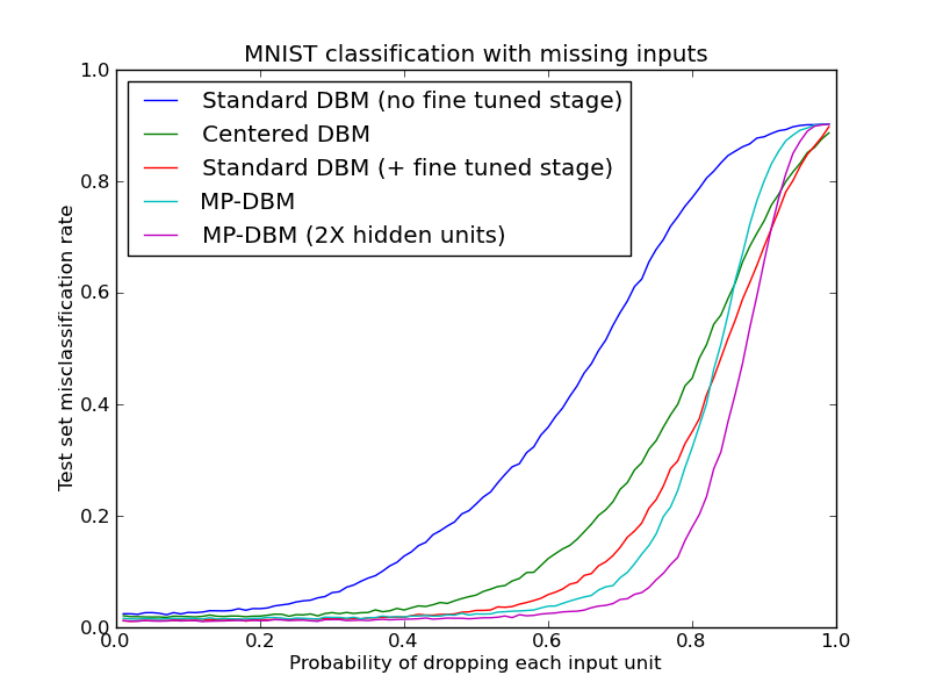
The original DBM was motivated primarily as a generative model with a high AIS score and as a classifier. Here we explore some more uses of the DBM as a generative model. First, we evaluate the use of the DBM to classify in the presence of missing inputs. See Fig. 7 for details. We find that for most amounts of missing inputs, the MP-DBM classifies better than the standard DBM or the best centering DBM. We also explored the ability of the DBM to resolve queries about random subsets of variables. See Fig. 8 for details. Again, we find that the MP-DBM outperforms the other DBMs.

This paper has demonstrated that MP training and the multi-inference trick provide a means of training a single model, with a single stage of training, that matches the performance of standard DBMs but still works as a general probabilistic model, capable of handling missing inputs and answering general queries. In future work, we hope to obtain state of the art performance by combining MP training with dropout, and also to apply this method to other datasets.

References

- Arnold and Ollivier (2012) Arnold, L. and Ollivier, Y. (2012). Layer-wise learning of deep generative models. Technical report, arXiv:1212.1524.
- Goodfellow et al. (2013) Goodfellow, I. J., Courville, A., and Bengio, Y. (2013). Scaling up spike-and-slab models for unsupervised feature learning. IEEE, special issue on deep learning. (To appear).
- Hinton et al. (2012) Hinton, G. E., Srivastava, N., Krizhevsky, A., Sutskever, I., and Salakhutdinov, R. (2012). Improving neural networks by preventing co-adaptation of feature detectors. Technical report, arXiv:1207.0580.
- Le Roux and Bengio (2008) Le Roux, N. and Bengio, Y. (2008). Representational power of restricted Boltzmann machines and deep belief networks. Neural Computation, 20(6), 1631–1649.
- Montavon and Müller (2012) Montavon, G. and Müller, K.-R. (2012). Learning feature hierarchies with cented deep Boltzmann machines. CoRR, abs/1203.4416.
- Neal (2001) Neal, R. M. (2001). Annealed importance sampling. Statistics and Computing, 11(2), 125–139.
- Salakhutdinov and Hinton (2009) Salakhutdinov, R. and Hinton, G. (2009). Deep Boltzmann machines. In Proceedings of the Twelfth International Conference on Artificial Intelligence and Statistics (AISTATS 2009), volume 8.
- Stoyanov et al. (2011) Stoyanov, V., Ropson, A., and Eisner, J. (2011). Empirical risk minimization of graphical model parameters given approximate inference, decoding, and model structure. In Proceedings of the 14th International Conference on Artificial Intelligence and Statistics (AISTATS), volume 15 of JMLR Workshop and Conference Proceedings, pages 725–733, Fort Lauderdale. Supplementary material (4 pages) also available.
- Tieleman (2008) Tieleman, T. (2008). Training restricted Boltzmann machines using approximations to the likelihood gradient. In W. W. Cohen, A. McCallum, and S. T. Roweis, editors, ICML 2008, pages 1064–1071. ACM.
- Younes (1999) Younes, L. (1999). On the convergence of Markovian stochastic algorithms with rapidly decreasing ergodicity rates. Stochastics and Stochastic Reports, 65(3), 177–228.