Intensity fluctuations in bimodal micropillar lasers enhanced by quantum-dot gain competition
Abstract
We investigate correlations between orthogonally polarized cavity modes of a bimodal micropillar laser with a single layer of self-assembled quantum dots in the active region. While one emission mode of the microlaser demonstrates a characteristic s-shaped input-output curve, the output intensity of the second mode saturates and even decreases with increasing injection current above threshold. Measuring the photon auto-correlation function of the light emission confirms the onset of lasing in the first mode with approaching unity above threshold. In contrast, strong photon bunching associated with super-thermal values of is detected for the other mode for currents above threshold. This behavior is attributed to gain competition of the two modes induced by the common gain material, which is confirmed by photon crosscorrelation measurements revealing a clear anti-correlation between emission events of the two modes. The experimental studies are in excellent qualitative agreement with theoretical studies based on a microscopic semiconductor theory, which we extend to the case of two modes interacting with the common gain medium. Moreover, we treat the problem by an extended birth-death model for two interacting modes, which reveals, that the photon probability distribution of each mode has a double peak structure, indicating switching behavior of the modes for the pump rates around threshold.
I Introduction
Quantum dot – microcavities are a very attractive system to study quantum optical effects in the solid state [1]. Apart from research on fundamental light matter interaction in the weak and strong coupling regime of cavity quantum electrodynamics [2, 3, 4, 5, 6], they offer the possibility to investigate stimulated emission in a regime approaching the ultimate limit of a thresholdless laser based on a single zero-dimensional gain center [7]. Studies in this field include, e.g., technological works on optically and electrically pumped microlasers aiming at an increase of the -factor which expresses the fraction of spontaneous emission coupled into the lasing mode [8, 9, 10]. In high -microlasers it becomes increasingly difficult to identify the transition from spontaneous emission to stimulated emission at threshold via their input-output characteristics [11]. This issue has triggered comprehensive experimental and theoretical research activities on the photon statistics of emission in terms of intensity autocorrelation function in order to unambiguously identify the onset of stimulated emission at threshold [12, 13, 9, 14]. Moreover, the autocorrelation function is very beneficial to identify single quantum dot controlled lasing effects [15, 16, 17] and to reveal other intriguing effects such as correlations between individual photon emission events [18] and chaotic behaviour of feedback coupled microlasers [19].
The research efforts on microcavity lasers so far have focused mostly on emission features based on the interaction between a single laser mode and the quantum dot gain medium. Going beyond this standard investigations, micropillar lasers with a bimodal emission spectrum allow one to address the coupling of two orthogonal optical modes via the common gain medium which can lead to characteristic oscillations in the coherence properties [20] and an enhanced sensitivity on external perturbations in the presence of optical self-feedback [19].
In the present work, we perform a detailed experimental and theoretical analysis of the mode coupling and gain competition of bimodal, electrically pumped micropillar lasers. A convenient measure for the study of the statistical properties of the electromagnetic field emission is the set of intensity correlation functions:
| (1) |
where , with delay time and photon annihilation operators and of the mode and the mode , correspondingly. The gain competition is reflected in distinct differences in the input-output characteristic and the autocorrelation function of the two optical modes. Moreover, the crosscorrelation function can illustrate correlations between emission events from the two modes. In order to describe and analysis these specific features of bimodal microlasers we extend the microscopic semiconductor model [13] accordingly by taking mode interactions into account. Similarly, we extend a standard birth-death approach [21] for the description of bimodal lasers. While the microscopic semiconductor theory is applied to model the input-output characteristics, the intensity correlation functions of the laser and the gain competition between the two emission modes within a strict mathematical framework, the extended birth-death approach allows for a more intuitive understanding of the underlying photon statistics.
The paper is organized as follows. In section II the experimental results obtained from an electrically pumped, bimodal micropillar laser will be presented. Section III deals with the theoretical description of the experimental data and is divided into two subsections addressing a microscopic semiconductor theory, and an extended birth-death approach, respectively. The paper closes in section IV with a comparison of the experimental and theoretical results and a conclusion.
II Experiment
The electrically pumped micropillar lasers are based on planar AlAs/GaAs microcavity structures which includes an active layer consisting of a single layer of In0.3Ga0.3As. High resolution electron beam lithography, plasma enhanced etching and metal deposition have been applied to fabricate high quality electrically pumped microlasers. For more details on the sample processing we refer to Ref. [22]. The microlasers have been investigated at low temperature ( K) using a high resolution micro-electroluminescence (EL) setup. A linear polarizer in combination with a -wave-plate is installed in front of the entrance slit of the monochromator in order to perform polarization resolved measurements of the laser signal. The photon statistics of the emitted light has been studied by means of the measurement of the photon autocorrelation function , that has been carried out using a fiber coupled Hanbury-Brown and Twiss (HBT) configuration with a temporal resolution ps. The HBT configuration is coupled to the output slit of the monochromator which has a focal length of m. The interaction of the orthogonally polarized modes of the microlaser has been investigated by means of photon crosscorrelation measurements. For this purpose, the light emitted by the microlaser is split by a polarization-maintaining 50/50 beamsplitter and coupled into two monochromators ( m), each of which is equipped with a linear polarizer at the input slit and a fiber coupled single photon counting module at the output slit. This configuration allows us to perform polarization resolved crosscorrelation measurements with a spectral resolution of eV.

First, let us focus on the input-output characteristics of the microlaser. Due to slight asymmetry of the cross-section of the pillar and the ring-shaped contact the degeneracy of the fundamental mode in the pillar microcavity is lifted and two distinct linearly polarized modes are supported [23]. In this context, the spectral splitting and accordingly the overlap between the two modes plays an important role for the studies of emission of bimodal cavities. Figure 1 shows representative polarization resolved spectra of an electrically pumped bimodal microlaser at threshold (injection current, A). The two linearly polarized modes are split in energy by eV and have absorption limited -factors of (mode 1) and (mode 2) at the threshold. The input-output characteristic of the bimodal microlaser is presented in Fig. 2(a). We observe pronounced differences between the two modes: while mode shows a standard “s”-shaped input-output characteristic with a threshold current of about A, the intensity of mode saturates at and even drops down for injection currents exceeding . This behavior indicates a pronounced competition between the modes and which is mediated by the common QD gain material as it will be further elaborated in the following.

Further, to study the lasing features we extract the emission linewidths of the two modes and plot them as a function of the injection current in Fig. 2(b). The linewidths of the modes and have similar magnitude and decrease strongly at threshold which reflects enhanced temporal coherence in the lasing regime. Interestingly, while the linewidth of the mode stays at a resolution limited value of eV, a slight increase of the linewidth can be observed for the mode above = 3. This is in agreement with the decreasing emission intensity seen in Fig. 2(a), which indicates an increasing contribution of spontaneous emission in the mode at high injection currents.
In order to verify the interpretation of mode coupling in terms of gain competition, we have performed crosscorrelation measurements between the modes and at different injection currents. An illustration of such a measurement is presented in Fig. 2(e) for = 3. The cross-correlation function shows a pronounced dip at which indicates an anti-correlation between emission events from the two laser modes. The anti-correlated emission occurs at a characteristic timescale of ns. Figure 2(d) reveals that the crosscorrelation function strongly depends on the injection current. It is useful to note, that, as it is seen from Fig. 2 in the regime of certain injection currents above the threshold ( ), the intensity of mode decreases and the statistics of mode demonstrates strongly super-Poissonian behavior, whereas the anti-correlation between the modes is the strongest.
The interplay between the two emission modes is also accompanied by strong temporal intensity fluctuations which are identified by measuring the photon autocorrelation function of the two competing modes for different injection currents. The respective dependencies, i.e. and versus injection current, are plotted in Fig. 2(c), while Fig. 2(f) shows the autocorrelation function for = 3. The mode shows the typical maximum of around threshold, which indicates the transition from spontaneous emission to stimulated emission, where is lower than expected from theory due to the limited temporal resolution of the HBT [14]. In contrast, the autocorrelation function of the mode , increases strongly at the pump rates well above threshold and reaches a maximum value of at = 3. This value is significantly higher than , expected for thermal light and, therefore, can not be explained by standard photon statistics.
It is important to note, that similar statistical properties of the emission, i.e. strong super-Poissonian behavior for the weak mode, has been also observed for microlasers in the presence of an external mirror, where a delayed feedback of the emitted signal disturbs laser operation and leads to strong bunching for the weak mode [19].
III Theory
To develop a theoretical framework for the study of the coupled carrier-photon system in the bimodal cavity we consider two different theoretical approaches. In the first, a microscopic theory of light-matter interaction of semiconductor QDs with the cavity field is given, which allows the derivation of the equations of motion for quantities of interest. In the second approach, starting with the master equation, statistics of the photon distribution can be derived for the case of two-level carriers.
III.1 Microscopic Semiconductor Theory
To study the interaction of QDs with the electromagnetic field inside an optical bimodal microcavities we have extended the Microscopic Semiconductor Theory [13] to the case of two modes and photon crosscorrelation functions.
III.1.1 Physical Model
The Microscopic Semiconductor Theory allows for inclusion of many-body effects of the carriers and can be used to calculate correlations required to determine the statistics of the emission of microcavities with active QDs (for a review see, e. g., Ref. [24]). The calculations are based on the cluster expansion truncation scheme of the equations of motion for operator expectation values [25].
In what follows we assume that only two confined QD shells for both electrons and holes are relevant: whereas the resonant interaction with the electromagnetic field of the bimodal cavity is due to the coupling with the -shell transition, the carrier generation due to electrical pumping is to take place in the -shell. The assumption suits well also for an experimental situation, where the electrical pumping is to take place via injection of electrons and holes into the wetting layer and subsequent fast relaxation to the discrete electronic states of the QDs. Further, carrier-carrier and carrier-phonon scattering contributions to the dynamics are evaluated using a relaxation time approximation, where the relaxation towards quasi-equilibrium is given in terms of a relaxation rate [26].
To be more specific, let us consider a bimodal microcavity with the QDs as gain medium with the driving performed by the recombination of carriers in the valence and conduction bands. The Hamiltonian that governs the temporal evolution of the overall system can be given in the form
| (2) |
where is the single-particle contributions for conduction and valence band carriers with the energies ,
| (3) |
and the two-particle Coulomb interaction is given by [27]
| (4) |
In the above, () and () are fermionic operators that annihilate (create) a conduction-band carrier in the state and a valence-band carrier in the state , respectively. Further, the Hamiltonian of the electromagnetic field modes inside the cavity reads
| (5) |
where () is the bosonic annihilation (creation) operator of the th mode of the cavity.
The energy of interaction of the QDs with the electromagnetic field inside the cavity in dipole approximation can be given by:
| (6) |
where the approximation of equal wave-function envelopes for conduction- and valence-band states is used. Moreover, for simplicity the coupling strength is assumed to be real.
The Hamiltonian given by Eq. (2) together with Eqs. (3–6) determines the dynamical evolution of the carrier and field operators and, in particular, the time evolution for operator expectation values. The equations of motion for quantities of interest, as for example the average photon number in the cavity modes and the average electron population in the conduction and valence bands, have source terms that contain operator expectation values of higher order. In this way, the approach bears an infinite hierarchy of equations of motion for various expectation values for photon and carrier operators. To perform a consistent truncation of the equations the cluster expansion scheme is applied (for details, see Ref. [13] and references therein). Namely, starting from the expectation values of the first order of photon operators, the equations of motion for operator expectation values are replaced by equations of motion for correlation functions. For example, instead of the equations of motion for expectation values of amplitudes of the cavity mode operators , the equations of motion for corresponding amplitude correlation functions are used. Then, to achieve a consistent classification and inclusion of correlations up to a certain order the truncation of the equations for correlation functions rather than for expectation values is performed.
In particular, in the case of a system without coherent external excitation and hold. Therefore, applying rotating-wave approximation here and thereafter, Heisenberg equations of motion for amplitude correlation functions of the mode operators can be given by
| (7) |
where is the loss rate of the th cavity mode and , with being the total number of QDs. Note, that both cavity-mode amplitude correlation functions and the coupled photon-assisted polarization amplitude correlations and are classified as doublet terms in the cluster expansion scheme, i.e., they correspond to an excitation of two electrons (four carrier operators). The equation of motion for the photon-assisted polarization amplitude correlation read [see also Eq. (15) in Appendix A]:
| (8) |
where is the detuning of the th cavity-mode from the QD transition and is a phenomenological dephasing parameter describing spectral line broadening. In the case of a bimodal cavity only the cavity modes with indices are resonantly coupled to the QDs. Whereas the modes with are not within the gain spectrum of the QD ensemble or have low -value. Since the population of the non-lasing modes and the cross-correlation functions and with remain negligibly small, the third terms on the right-hand side of Eq. (8) can be effectively set equal to zero. Thus, Eq. (8) for can be solved in the adiabatic limit yielding a time constant that describes the spontaneous emission into non-lasing modes according to the Weisskopf-Wigner theory. The spontaneous emission of QDs into non-lasing modes leading to a loss of excitation is described by -factor defined as the ratio of the spontaneous emission rate into the lasing modes and the total spontaneous emission rate enhanced by the Purcell effect :
| (9) |
The dynamics of carrier population of the electrons in the -shell is given by
| (10) |
Here, the first term on the right-hand side originates from the interaction with the cavity-modes, the second term describes the relaxation of carriers from the - to the -shell with a relaxation timescale and the term represents the loss of excitation into the non-lasing modes.
Further, we assume, that the -shell carriers are generated at a constant pump rate . Then, similar to Eq. (10), the equation of motion for the carrier population of the electrons in the -shell reads:
| (11) |
where the last term on the right-hand side describes spontaneous recombination of -shell carriers. The corresponding equations for valence band carriers are relegated into Appendix A.
The form of the expression for the intensity correlation functions suggests [see Eq. (1)] that to exploit the statistical properties of the light emission using intensity correlations, a consistent treatment within the cluster expansion up to the quadruplet order is required. In particular, the equations of motion for cavity-mode intensity correlations read:
| (12) |
The equations of motion for further correlation functions of the quadruplet order, which include correlation between the photon-assisted polarization and the photon number, can be found in Appendix A [see Eqs. (18)–(21)].
III.1.2 Results
As described above, the quadruplet order of the cluster expansion leads to a system of coupled equations [see Eqs. (7)–(8), (10)–(11), (12) together with Eqs. (15)–(21)]. The system of differential equations describe the dynamics of various correlations between carriers and cavity modes. In particular, the method makes it possible to obtain both amplitude and intensity correlation functions of the cavity emission modes including the effects of the carrier-photon correlations and the many-body Coulomb interaction.
In the ensuing section the numerical analysis of the time evolution of the emission correlation functions is presented. To relate our theory to the experimental results we estimate the number of QDs with effective gain contribution by starting with the initial density of present QDs and excluding the ones with negligible spectral and spatial overlap. Thus, it is assumed that the cavity mode field is coupled to identical QDs. Further, we consider continuous carrier generation in the -shell at a constant rate as an excitation process.
To obtain a valid comparison with the experimental results we simulate the coupled system using numerical integration routines with a realistic set of parameters , , , , and . The number of carriers within the frequency region of interest is estimated from the total density of QDs to be . For the assumed the carrier recombination is determined by the stimulated emission into the lasing modes and with a characteristic time scale and into the non-lasing modes with a characteristic time scale that can be found from Eq. (9) for the given set of parameters. Further, we assume that the cavity mode is in exact resonance with the QD transition () and the mode is detuned with . In Fig. 3 we present the simulation results for intensity functions for the modes , , autocorrelation functions and crosscorrelation as a function of the pump power. Figure 3(a) reveals, that whereas the mode shows a drastic increase of emission intensity, the intensity of the emission mode reaches a maximum and then slowly decreases with increasing pump power in good agreement with the experimental data depicted in Fig. 2(a). The calculations further show, that, in agreement with the experimental data in Fig. 2(c), the dependencies of the autocorrelation functions for the cavity modes and on the pump power exhibit dramatically different behavior. As shown in Fig. 3(b) for low values of pump power, the autocorrelation function is equal to characteristic for the statistics of thermal light. For higher rates of the pump power, the autocorrelation function of the mode drops close to the value indicating the emission of coherent laser light. In contrast, the autocorrelation function of mode slightly decreases at first with increasing pump powers, but for larger values of the pump power, it increases and reaches values well above , which is in agreement with the behavior of the autocorrelation function detected in the experiment {see Fig. 2(c); recall the limited temporal resolution of the HBT [14]}. The gain competition behavior between the modes can be approved by plotting the crosscorrelation function [see Fig. 3(c)], that decreases to the values smaller than unity at the power pump values for which the lasing behavior of the mode is observed [also, compare to Fig. 2(d)]. Note, that the discrepancy of the experimental and theoretical results for the autocorrelation function of mode [Figs. 2(c) and 3(b), correspondingly] and the crosscorrelation function [Figs. 2(d) and 3(c), correspondingly] at the higher pump powers is due to the crosstalk between the modes, which cannot be completely avoided in the measurements.
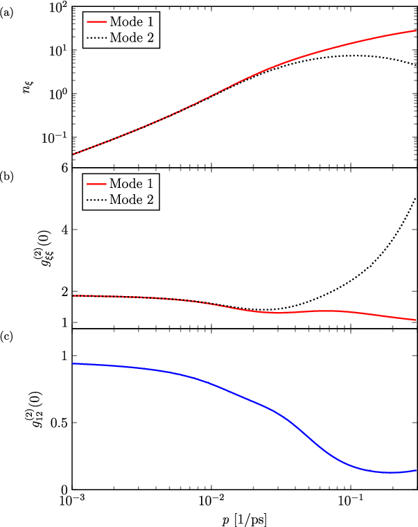
The numerical simulation of the cluster expansion truncation scheme of the quadruplet order can be approved by plotting the emission mode autocorrelation functions for higher order of truncation (not shown), which demonstrates qualitatively the same behavior of the functions independent of the order of truncation. It is important to note, that since the framework of the microscopic semiconductor theory presented in this section is based on the truncation of the hierarchy of equations for correlation function, the numerical results are valid in the regime when higher order correlations remain small. As it can seen from the numerical evaluation of the truncated equations, this is not the case for pump power rates exceeding , where the correlation functions strongly increase. To get a deeper understanding of the statistical properties of the emission in the next section we will use a different approach to gain insight into the full photon statistics.
III.2 Extended Birth-Death Approach
In the following subsection we present an alternative approach to the study of the light-matter interaction of QDs with a bimodal cavity, that involves numerically solving a complete master equation and thus deriving the time evolution of the system. In contrast to the Microscopic Semiconductor Model discussed in detail in Sec. III.1, the approach allows to calculate not only photon auto- and crosscorrelation-functions but also full photon statistics. We follow the Rice and Carmichael approach (see Ref. [21]) and extend it to the case of a bimodal cavity with two resonant modes containing and photons, respectively. The method simplifies the model for the gain medium and takes into account only fully inverted two-level systems. Note, that no semiconductor effects or complex level structure are reflected. The state of the gain medium is fully described by the number of excited carriers . A detailed discussion of the master equation approach, the semiclassical rate equations and its connection to the semiconductor theory for the case of a single-mode microcavity can be found in Refs. [13, 28] and references therein. The master equation describes the time evolution of the diagonal elements
| (13) |
of the density matrix . These elements can be interpreted as the probability of finding a state with , photons in the modes and , respectively, and Atoms in the excited state.
III.2.1 Physical Model
To arrive at the final form of the master equation a birth and death model, analogue the one introduced by Rice and Carmichael [21], is considered. Transition rates into and out of the state are connected to the relevant processes in the coupled photon carrier system. Figure 4 shows how the master equation is derived on a phenomenological level. The filled circles represent a state with excited carriers, and photons in the cavity modes, i.e. the diagonal elements of the density matrix. The photon distribution for mode is gained by summation over the remaining indices . Figure 4(a) illustrates the coupling of one mode to the gain medium. The horizontal axis shows the number of photons in mode and the vertical axis shows the number of excited carriers . The carrier generation is represented by solid vertical arrows since the photon number is not changed. The rate of carrier generation in the excited level is given by the pump power . Vertical dotted arrows indicate the loss of excited carriers due to spontaneous emission into non lasing modes. Moreover, the emission into the cavity modes is represented by pairs of diagonal arrows corresponding to spontaneous (dotted arrow) and stimulated (solid arrow) emissions, since an excited carrier is lost and one photon in one of the modes is gained. The factors and are introduced, which represent the fractions of laser emission rate into the cavity modes and , correspondingly, where the relation holds. Further, the interaction of the modes is illustrated in Fig. 4(b). The two axes show the number of photons , in the modes and , respectively. The horizontal and vertical dotted arrows represent the cavity losses of the two lasing modes with the loss rates . A phenomenological nonlinear coupling between the lasing modes and mediated by the gain medium is also introduced. In contrast to the Microscopic Semiconductor Theory (see Sec. III.1), where the coupling between the cavity modes is mediated by the overlap of the mode functions with the gain carriers, here a nonlinear coupling between the lasing modes and is introduced phenomenologically. The mode coupling strengths and are represented by the diagonal solid arrows in the sketch and play the role of the detuning between the modes used in Sec. III.1. The complete master equation derived by the phenomenological birth and death model reads:
| (14) |
In the above, each line corresponds to a process in the coupled carrier photon system, i.e. to arrows going in and out of a state in Fig. 4.
(a)

(b)

III.2.2 Results
The stationary solution of Eq. (14) gives the photon probability distribution. Figure 5 shows the photon distributions for various pump strengths. Above the laser threshold the autocorrelation functions of the modes and are quite different, while drops to values close to one indicating Poissonian statistics, rises up to values substantially larger then two (thermal statistics). The results for the autocorrelation functions of the modes and are in full agreement with the ones obtained within the Microscopic Semiconductor Theory in Sec. III.1 (see e.g. Fig. 3). However, in contrast to the experimental data presented in Fig. 2, the autocorrelation function of the mode monotonically increases also for high pump power rates.
The full photon statistics reveals that both mode statistics exhibit a double peak structure. The first peak appears at the zero photon state declining very steep and a second Poissonian like peak appears at the higher photon states. In the mode the Poissonian peak is very pronounced and dominates the statistics, the mode is dominated by the first peak at zero photon number states. These statistics combined with the fact of a crosscorrelation function far below unity allows for the interpretation of a switching behavior of the modes. Both modes are in a superposition of a lasing and a non lasing state and are alternating in between them.
(a)

(b)

IV Discussion and Conclusions
We have investigated laser emission of electrically pumped quantum dots in a bimodal micropillar cavity with special emphasis to the effects induced by gain competition of the two orthogonally polarized modes.
The system consisting of a single low-density layer of QDs and two spectrally splitted but overlapping modes with nearly equal -factors, induced from the double degenerate fundamental mode by slight cross-section asymmetry of the pillar, represents a viable platform for the study of the coupling of two cavity modes in the presence of a common gain medium. The polarization resolved measurements of the statistical properties of the emitted light reveal, that the two competing modes display completely different features. One of the modes (mode ) demonstrates typical statistical behavior of a laser mode, namely the mode intensity displays the usual ”s”-shaped input-output characteristic, and the autocorrelation function at zero time delay, measured using a HBT setup, indicates the transition from spontaneous to stimulated emission for increasing pump rates. The measurements of the input-output characteristic of mode indicate the threshold behavior, but for further increasing pump rates the intensity saturates and even decreases, as the result of the competition of the two modes induced by the common gain material. Moreover, the autocorrelation function at zero time delay of mode at certain pump rates higher than the threshold values exhibits intensity fluctuation much higher than for a thermal state. It is worth to note, that at these rates of the injection current the anti-correlation between the two modes is the strongest. For even larger pump rates, the crosstalk between the modes induces a reduction of the autocorrelation function at zero time delay of the mode reaching the value for a lasing mode. Similarly, at these pump rates the crosscorrelation measurements indicate increasing correlation between the modes due to the crosstalk.
The experimental results have been supported by the theoretical calculations within the framework of the Microscopic Semiconductor Theory [13], which we have extended to the case of two cavity modes interacting with the QD-gain medium. Using the cluster expansion scheme for correlation functions, we have obtained the emission statistics of the carrier-photon system in the bimodal cavity, taking into account the many-body effects. Importantly, within our approach the effects related to the coupling of the two modes of the bimodal cavity, induced by the interaction with the common QD carriers are consistently included on the microscopic level. The solution of the equations of motion for correlation functions reveals, that indeed the autocorrelation function of the mode for the pump rates larger than the threshold rate reaches values well above , that corresponds to the thermal state of light. The decrease of the crosscorrelation function of the two modes below unity indicates anti-correlated behavior of the mode coupling at these pump rates. In fact, this effect can be explained by random intensity switching between the two modes, which has negligible influence on the photon statistics of the lasing mode, but strongly affects the mode for which the relative strength of fluctuations is larger. It is worth to mention, that in the case of macroscopic two-mode ring lasers [29] large intensity fluctuations have been also found in the statistics of the more lossy mode, as the result of the mode competition with the favored mode and emission switching of the common atomic ensemble.
To complement the theoretical results with the photon-number statistics and to provide an interpretation to the super-thermal intensity fluctuations of mode , we have extended the birth-death model of the master equation to the case of a bimodal cavity. In particular, we have assumed a phenomenological nonlinear coupling between the cavity modes, mediated by the overlap of the modes with the gain carriers. In this way, solving the complete master equation, we have shown, that the photon number statistics of the both modes exhibit similar double peak structure—a peak at the zero photon state and a second peak at a higher photon number. The results imply, that the both modes are in a superposition of a lasing state and a thermal-like state. Whereas, the Poisson peak at the higher photon number dominates the statistics of the mode , the statistics of the mode indicates thermal state-like behavior, with a pronounced peak at zero photon state complemented with a local maximum at a higher photon number state. Thus, we may conclude that the photon number distribution of the two modes approves the switching behavior of the interaction of the two modes with the common gain medium.
Similar double peak curve has been also observed in a semiclassical approach for the intensity probability distributions of the both modes of ring lasers [29], where the nonzero values of the light intensity are much more probable than the zero values for the favored mode and the other way around for the lossy mode. Moreover, a double peak structure of the photon number distribution has been found for the composite mode at threshold in the two-mode open laser theory [30], where both modes interact with the common ensemble of atoms and with the common dissipation system.
V Acknowledgment
This work was financially supported by the Deutsche Forschungsgemeinschaft within the research grants RE2974/2-1 and Wi1986/3-1 and the State of Bavaria. The authors gratefully thank M. Emmerling and A. Wolf for expert sample preparation. A. Foerster acknowledges financial support from the Graduiertenförderung Sachsen-Anhalt.
Appendix A Equations for Microscopic Semiconductor Model
In this Appendix we present the equations of motion that together with Eqs. (7), (8), (10), (11) and (12) complete the full set of equations of motion for one-time correlation functions on the quadruplet level of the cluster expansion:
| (15) |
| (16) |
| (17) |
| (18) |
| (19) |
| (20) |
| (21) |
References
- [1] S. Reitzenstein, IEEE J. Sel. Top. Quantum Electron. 18, 1733 (2012).
- [2] J. M. Gérard, B. Sermage, B. Gayral, B. Legrand, E. Costard, and V. Thierry-Mieg, Phys. Rev. Lett. 81, 1110 (1998).
- [3] M. Bayer, T. L. Reinecke, F. Weidner, A. Larionov, A. McDonald, and A. Forchel, Phys. Rev. Lett. 86, 3168 (2001).
- [4] K. J. Vahala, Nature 424, 839 (2003).
- [5] J. P. Reithmaier, G. Sek, A. Löffler, C. Hofmann, S. Kuhn, S. Reitzenstein, L. V. Keldysh, V. D. Kulakovskii, T. L. Reinecke, and A. Forchel, Nature 432, 197 (2004).
- [6] T. Yoshie, A. Scherer, J. Hendrickson, G. Khitrova, H. M. Gibbs, G. Rupper, C. Ell, O. B. Shchekin, and D. G. Deppe, Nature 432, 200 (2004).
- [7] S. Noda, Science 314, 260 (2006).
- [8] W. H. Wang, S. Ghosh, F. M. Mendoza, X. Li, D. D. Awschalom, and N. Samarth, Phys. Rev. B 71, 155 (2000).
- [9] S. Strauf, K. Hennessy, M. T. Rakher, Y.-S. Choi, A. Badolato, L. C. Andreani, E. L. Hu, P. M. Petroff, and D. Bouwmeester, Phys. Rev. Lett. 96, 127404 (2006).
- [10] S. Reitzenstein, C. Böckler, A. Bazhenov, A. Gorbunov, A. Löffler, M. Kamp, V. Kulakovskii, and A. Forchel, Opt. Express 16, 4848 (2008a).
- [11] G. Björk, A. Karlsson, and Y. Yamamoto, Phys. Rev. A 50, 1675 (1994).
- [12] P. R. Rice and H. J. Carmichael, Phys. Rev. A 50, 4318 (1994a).
- [13] C. Gies, J. Wiersig, M. Lorke, and F. Jahnke, Phys. Rev. A 75, 013803 (2007).
- [14] S. M. Ulrich, C. Gies, S. Ates, J. Wiersig, S. Reitzenstein, C. Hofmann, A. Löffler, A. Forchel, F. Jahnke, and P. Michler, Phys. Rev. Lett. 98, 043906 (2007).
- [15] Z. G. Xie, S. Götzinger, W. Fang, H. Cao, and G. S. Solomon, Phys. Rev. Lett. 98, 117401 (2007).
- [16] S. Reitzenstein, T. Heindel, C. Kistner, A. Rahimi-Iman, C. Schneider, S. Höfling, and A. Forchel, Appl. Phys. Lett. 93, 061104 (2008b).
- [17] M. Nomura, N. Kumagai, S. Iwamoto, Y. Ota, and Y. Arakawa, Opt. Express 17, 15975 (2009).
- [18] J. Wiersig, C. Gies, F. Jahnke, M. Aßmann, T. Berstermann, M. Bayer, C. Kistner, S. Reitzenstein, C. Schneider, S. Höfling, A. Forchel, C. Kruse, J. Kalden, and D. Hommel, Nature 460, 245 (2009).
- [19] F. Albert, C. Hopfmann, S. Reitzenstein, C. Schneider, S. Höfling, L. Worschech, M. Kamp, W. Kinzel, A. Forchel, and I. Kanter, Nature Communications 2, 233 (2011).
- [20] S. Ates, S. M. Ulrich, P. Michler, S. Reitzenstein, A. Löffler, and A. Forchel, Appl. Phys. Lett. 90, 161111 (2007).
- [21] P. R. Rice and H. J. Carmichael, Phys. Rev. A 50, 4318 (1994b).
- [22] S. Reitzenstein, T. Heindel, C. Kistner, F. Albert, T. Braun, C. Hopfmann, P. Mrowinski, M. Lermer, M. K. C. Schneider, S. Höfling, and A. Forchel, IEEE J. Quantum Elect. 17, 1670 (2011).
- [23] S. Reitzenstein, C. Hofmann, A. Gorbunov, M. Strauß, S. H. Kwon, C. Schneider, A. Löffler, S. Höfling, M. Kamp, and A. Forchel, Appl. Phys. Lett. 90, 251109 (2007).
- [24] C. Gies, J. Wiersig, and F. Jahnke, in Single Semiconductor Quantum Dots, NanoScience and Technology, edited by P. Michler (Springer Berlin Heidelberg, 2009) pp. 1–30.
- [25] J. Fricke, Ann. Phys. 252, 479 (1996).
- [26] T. Nielsen, P. Gartner, and F. Jahnke, Phys. Rev. B 69, 235314 (2004).
- [27] N. Baer, C. Gies, J. Wiersig, and F. Jahnke, Eur. Phys. J. B 50, 411 (2006).
- [28] C. Gies, Theory for light-matter interaction in semiconductor quantum dots, Ph.D. thesis, Universität Bremen (2008).
- [29] S. Singh and L. Mandel, Phys. Rev. A 20, 2459 (1979).
- [30] V. Eremeev, S. E. Skipetrov, and M. Orszag, Phys. Rev. A 84, 023816 (2011).