On differentiability of volume time functionsThanks: Preprint UWThPh-2013-1

In his classical work on domains of dependence and global hyperbolicity [14] Geroch showed how to construct a time function, namely a continuous function increasing over every future directed causal curve, by considering a weighted volume of the chronological past of the point. This strategy was extended by Hawking [17, 18] who proved that in a stably causal spacetime it is possible to obtain a time function through suitable averages of Geroch’s volume functions (see [29, 13, 8, 25] and references therein for alternative constructions). Nevertheless, even in the globally hyperbolic case the differentiability properties of the resulting functions do not seem to have been properly understood so far.¹¹ 1 The reader is referred to [28, 8] for a review of the history of the problem. The object of this note is to establish differentiability of a large class of volume functions under the hypothesis of global hyperbolicity, as well as smoothability of a class of time functions for stably causal space-times. Indeed, assuming global hyperbolicity, at the end of Section 3 below we prove:

Following Geroch, we can now define $\tau_{\varphi}=\ln(\tau^{-}_{\varphi}/\tau^{+}_{\varphi})$ so that if $\gamma$ is an inextendible causal curve then $\tau_{\varphi}\circ\gamma$ is onto $\mathbb{R}$. As a consequence, the differentiability of $\tau_{\varphi}$ implies that the level sets of $\tau_{\varphi}$ are Cauchy spacelike hypersurfaces (thus not just acausal and Lipschitz).

In view of the analysis in [20] it is conceivable that the functions $\tau_{\varphi}^{\pm}{}$ are $C^{1,1}$, but we have not investigated the issue any further, as we will smooth out these functions in any case, see Corollary 5.6 below. The smoothing procedure will establish the existence of smooth Cauchy time functions in globally hyperbolic spacetimes. This result, already obtained in [7, 6, 13] by different means, plays a key role in the theory as it implies that Geroch’s topological splitting [18] can actually be chosen smooth.

Some comments on the proof might be in order. We write a light-cone integral formula for a candidate derivative of $\tau_{\varphi}^{\pm}{}$. The integrand involves Jacobi fields which might be blowing up as one approaches the end of the interval of existence of the geodesic generators of

So the weighting function $\varphi$ has to compensate for this, which provides one of the constraints on the set of admissible functions $\varphi$. In particular, we are going to introduce an auxiliary complete Riemannian metric $h$ in order to control and obtain a sufficiently fast fall-off of $\varphi$ at infinity.

An interesting feature of our candidate formula for the derivative of $\tau_{\varphi}^{\pm}{}$ is that it involves an integral on just $E^{\pm}(p)$, and not on the whole light cone issued from $p$. As a consequence, most of the pathological behavior connected with non-differentiability of the exponential map after conjugate points is avoided.

Now, the domain of integration that interests us is generated by lightlike geodesics that may be either complete or incomplete. The distinction between completeness and incompleteness is, however, rather unimportant since, without loss of generality, we may conformally rescale $g$ so as to make all the null geodesics complete [2]. Next, there might exist generators that do not meet the cut-locus and which span an area region on $E^{\pm}(p)$ that does not vary continuously with $p$. (Example: Let $(N,g)$ be any bounded globally hyperbolic subset of two-dimensional Minkowski spacetime, with the weighting function $\varphi$ in (1.1) equal to one. Let $q\in N$ and set $M=N\setminus J^{-}(q)$, with the induced metric. Then $\tau_{\varphi}^{-}{}$ is not differentiable at the boundary of the future of $q$; see Figure 1.)

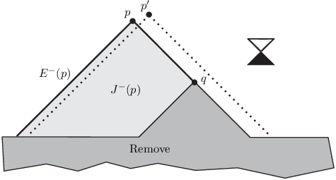
It turns out that the discontinuous behavior illustrated by the example happens “close to infinity” in the complete auxiliary metric, where a fast fall-off of $\varphi$ amends the problem.

In Section 4 we show that a local application of our integral formula gives a simple proof of the anti-Lipschitz character of $\tau_{\varphi}^{\pm}{}$ along causal curves. We also show that the anti-Lipschitz condition with respect to a spacetime metric with wider light cones allows us to smooth the time function. This result is used to prove the smoothability of Hawking’s time function in stably causal spacetimes, and to prove the existence of smooth Cauchy time functions in globally hyperbolic spacetimes, by taking advantage of the stability of global hyperbolicity. We also prove the equivalence between stable causality and the existence of a time function by taking advantage of the equivalence between the former property and $K$-causality.

Finally, in the last section we prove that we can dispense with the result on the stability of global hyperbolicity, and prove directly the smoothability of Geroch’s Cauchy time functions, by showing that every Lipschitz and anti-Lipschitz time function is in fact anti-Lipschitz with respect to a spacetime metric with wider light cones.

To avoid ambiguities, we start by noting that our signature is $(-,+\cdots+)$, and that we use a convention in which the zero vector is not a null vector. Space-times of any dimension $n+1$, $n\geq 1$, are allowed, though it must be said that the case $n=1$ is rather simpler than the remaining dimensions, as there are then no null conjugate points.

The proof of Theorem 1.1 will require some understanding of the null cut-locus. For this, we start by recalling some definitions and results from [3], see especially Sections 9.2 and 10.3 there.

Our spacetime metric $g$ will be $C^{2,1}$ throughout the paper. This condition assures the existence of convex neighborhoods, continuous differentiability of the exponential map and Lipschitzness of the Riemann tensor. These conditions can possibly be weakened.

The past Lorentzian distance function

is defined as

where the $\sup$ is taken over all past-directed causal curves from $p$ to $q$. In general smooth spacetimes the function $d_{L}^{-}$ is lower semi-continuous [3], while for globally hyperbolic (smooth) spacetimes it is finite and continuous. Moreover, we observe that the arguments in [10, 3] can be used to prove these results for $C^{2}$ metrics. (For more on the continuity properties of the Lorentzian distance function under low causality conditions see [23].)

Throughout this paper we choose once and for all a smooth complete Riemannian metric $h$ on ${\mycal M}$. We denote by $N^{-}_{h}{\mycal M}$ the bundle of past-directed $h$-unit $g$-null vectors. A curve will be said to be $h$-parametrised if it is parametrised with arc-length measured with the metric $h$.

Sometimes, for simplicity, we shall speak of geodesics though strictly speaking we should speak of pregeodesics, namely when the curve is a geodesic up to the parametrization. We will say that $\gamma$ is a half-geodesic if $\gamma$ satisfies the geodesic equation and if $\gamma\colon[0,a)\to{\mycal M}$ is maximally extended in the direction of increasing parameter. If $\gamma$ is parametrised by $h$-arc length with respect to a complete Riemannian metric, then $a=\infty$ (see, e.g., [10, 22, 3]).

For any past-directed null half-geodesic $\gamma\colon[0,\infty)\to{\mycal M}$ parametrised by $h$-arc length we set

The points of $E^{-}(p)$ which are sufficiently close to $p$ are connected to $p$ by achronal geodesics starting at $p$. We now define a subset $\mathring{E}^{-}(p)$ through a union of lightlike geodesic segments as follows

If $({\mycal M},g)$ is globally hyperbolic and if $t_{-}(\gamma)<\infty$, then the point $\gamma(t_{-}(\gamma))$ is either conjugate to $\gamma(0)$ along $\gamma$ and/or there exist two distinct null achronal geodesics from $\gamma(0)$ to $\gamma(t_{-}(\gamma))$ (see [3, Theorem 9.15], compare the arguments in the proof of Proposition 2.1). The points $\gamma(t_{-}(\gamma))$ are end points of generators of past light-cones [4]. The set of end points of past-directed generators starting at $p$ is called the past null cut-locus of $p$. It is known, in spacetime dimension $n+1$, that the past null cut-locus of $p$ has vanishing $n$-dimensional measure within $\exp_{p}(\mathbb{R}(N_{h}^{-})_{p}{\mycal M})$. (This fact also follows from Fubini’s theorem and Proposition 2.1 below; compare the proof of Lemma 3.1.) (The result is of course trivial in $1+1$ dimensions.)

For a $C^{2,1}$ metric $g$, the set $\mathring{E}^{-}(p)$ is a $C^{1,1}$ null hypersurface, indeed it is an immersion by the local injectivity of the exponential map away from conjugate points, and it is an embedding because there are no self intersections as we remove the points of the light cones behind the cut points and the cut points themselves. In a globally hyperbolic spacetime

We can parameterize the set of all maximally extended past-directed half-geodesics by the initial positions and $h$-normalised tangent vector at the starting point. In other words, such half-geodesics are in one-to-one correspondence with vectors in $N^{-}_{h}{\mycal M}$. This induces in the obvious way a topology on the set of half-geodesics. We have:

Passing to another subsequence if needed, by global hyperbolicity there exists a causal past-directed half-geodesic $\sigma$ such that $\sigma_{i}(s)\to\sigma(s)$ for $s\in[0,\infty)$, with the sequence $\{\widetilde{t}_{i}\}_{i\in\mathbb{N}}$ convergent, and $\sigma_{i}(\widetilde{t}_{i})\to\gamma(t)$. If $\sigma$ and $\gamma$ are distinct, it follows that $t\geq t_{-}(\gamma)$, as desired. If $\sigma$ and $\gamma$ coincide but $t$ is larger than or equal to the distance to the first conjugate point of $\gamma(0)$ along $\gamma$ we again obtain $t\geq t_{-}(\gamma)$, and we are done.

It remains to consider the possibility that $\sigma$ and $\gamma$ coincide and that $t$ is smaller than the $h$-distance (possibly infinite, if $t_{-}(\gamma)=\infty$) to the first conjugate point along $\gamma$ of $\gamma(0)$. For $X\in T{\mycal M}$ let $\gamma_{X}$ denote a half-geodesic such that $\dot{\gamma}_{X}(0)=X$. By continuity of $\det\exp_{*}$, there exists a neighborhood ${\mycal O}$ of $\dot{\gamma}(0)$ in $T{\mycal M}$ such that for every causal vector $X\in{\mycal O}$ and every past-directed half-geodesic $s\mapsto\gamma_{X}(s)$ the $h$-distance along $\gamma_{X}$ to the first conjugate point of $\gamma_{X}(0)$ is larger than $t$. This contradicts $t_{-}(\gamma_{i})<t$ thus this case does not really apply. Hence, $t_{-}$ is lower semi-continuous, and thus also continuous, as desired. ∎

In this section we assume that $({\mycal M},g)$ is a globally hyperbolic spacetime and show that the functions $\tau_{\varphi}^{\pm}{}$, as defined in equation (1.1), are differentiable for suitably chosen $\varphi$. We consider only $\tau_{\varphi}^{-}{}$, the result for $\tau_{\varphi}^{+}{}$ follows by changing time-orientation. We will always assume that $\varphi$ is continuous and non-negative. We start by assuming that $\varphi$ has compact support.

Let $p\in{\mycal M},$ and let

be any future-directed, timelike $h$-arc length parametrised curve passing through $p=\gamma(0)$. Choose a $g$-orthonormal frame at $p$, and parallel-propagate the frame along $\gamma$. This defines $g$-orthonormal frames $\{e_{\mu}(s)\}$ at $\gamma(s)$. We will say that $g$-geodesics at different points of $\gamma$ are pointing in the same direction if the frame components of their initial velocities in the frame $\{e_{\mu}(s)\}$ coincide, i.e. if their tangent vectors at $\gamma$ are parallel transports of each other along $\gamma$. Then, for each generator of $\mathring{E}^{-}(p)$, we may associate a family of half-geodesics, parametrised by $s\in\mathbb{R}$, that emanate from the point $\gamma(s)$ with initial tangent vector pointing in the same direction as the chosen generator. Thus, points on neighbouring light-cones with vertices on $\gamma$ can be obtained by flowing along the associated Jacobi fields. This explains the construction that follows.

Let $\tau\mapsto\Gamma_{s}(\tau)$ be any past-directed affinely parametrised null half-geodesic starting at $\gamma(s)$, where $\tau\in[0,\tau_{-}(s))$ , with $\Gamma_{s}(\tau_{-}(s))$ the cut point of $\Gamma_{s}$. Its tangent vector $\frac{d}{d\tau}$ at $\gamma(s)$ is extended all over $\gamma$ through parallel transport, i.e.

over $\gamma$. Taking this parallel tangent vector field as initial data in the geodesic equations, the definition of $\Gamma_{s}$ is extended to different values of $s$. It is well known that by the local injectivity of the exponential map away from conjugate points, $\tau_{-}(s)$ is lower semi-continuous, thus the pairs $(s,\tau)$, $s\neq 0$, for which $\Gamma$ is defined form an open set. The mapping $\Gamma(s,\tau)=\Gamma_{s}(\tau)$ is generated by past-directed lightlike half-geodesics with initial endpoint $\gamma(s)$ at $\gamma$ and is really an embedding (surface). Indeed, two geodesics generators relative to different values of $s$ cannot intersect, namely it cannot be $\Gamma_{s^{\prime}}(\tau^{\prime})=\Gamma_{s}(\tau)$ for $s^{\prime}>s$, otherwise it would be possible to go from $\Gamma_{s^{\prime}}(\tau^{\prime})$ to $\gamma(s^{\prime})$ with a timelike curve in contradiction with the fact that $\Gamma_{s^{\prime}}(\tau^{\prime})$ stays before the cut point of $\Gamma_{s^{\prime}}$. Similarly, the image of $\Gamma$ cannot develop focusing points, for this would imply that a certain Jacobi field $X$ to be introduced in a moment vanishes, a fact which we prove to be impossible.

Since $(s,\tau)$ provide coordinates over the image of $\Gamma$, we have that

commute near $\gamma$, thus

over $\gamma$. Now, observe that $X$ is the variational field of $\Gamma_{s}(\tau)$, where the longitudinal curves are geodesics. Thus it is a Jacobi field whose value at $\gamma(s)$ is $\dot{\gamma}(s)$, while its first covariant derivative vanishes thanks to the mentioned commutation relation. It is interesting to observe that, since $X$ is Jacobi, for every fixed $s$ we have that $\tau\mapsto g(X,\frac{d}{d\tau})$ is an affine function of $\tau$ over $\Gamma_{s}(\tau)$, a fact which, given the initial conditions, implies that $g(X,\frac{d}{d\tau})$ is a constant whose value can be inferred from its value at the tip $\gamma(s)$. In particular, since $\dot{\gamma}$ is future-directed and timelike, $g(X,\frac{d}{d\tau})$ is positive over $\Gamma_{s}$ so, as anticipated, there cannot be focusing points due to the variation of coordinate $s$, although, of course, each individual light cone for fixed $s$ might develop a conjugate point at or after the cut point and hence outside the restricted $\tau$-domain $[0,\tau_{-}(s))$. We conclude that the image of $\Gamma$ is really a surface. Observe that since $X$ does not vanish it can even be defined at the cut point. However, by changing the generator ending at the endpoint (and $\Gamma$) one would get a different value of $X$. This fact will play no significant role in what follows due to the fact that the set of cut points has negligible measure.

So far $X$ has been defined over the surface defined by the mapping $(s,t)\mapsto\Gamma(s,\tau)$. By taking generators of $\mathring{E}^{-}(\gamma(s))$ with starting tangent vector having different components with respect to the base $\{e_{\mu}\}$ we obtain a vector field defined over $\cup_{s}\mathring{E}^{-}(\gamma(s))$.

As the Riemann tensor is Lipschitz, and since $X$ satisfies the Jacobi equation, by using the dependence on initial conditions of first order ODEs we have that the vector field $X$ is Lipschitz, a fact to be used below.

Let ${\mycal U}$ be any relatively compact domain containing the support of $\varphi$. Consider the map $\hat{L}\colon T{\mycal M}\to\mathbb{R}$ defined as

where $L(Z)$ is the Jacobi field $X$ over $E^{-}(\pi(Z))$ obtained as the solution of the Jacobi equation over each generator by imposing, (a) $L(Z)=Z$ at $\pi(Z)$, and (b) a vanishing derivative at $\pi(Z)$ in the direction of the affinely parametrised generator: $\frac{D}{d\tau}L(Z)|_{\tau=0}=0$.

The field $L(Z)$ is linear in $Z$ and hence at each point depends continuously on $Z$. Moreover, by Proposition 2.1 the sets $\partial(\mathring{E}^{-}(p))\cap{\mycal U}$, when non-empty, are continuous radial graphs which vary continuously with $p$. As the domain of integration $\mathring{E}^{-}(\pi(Z))\cap{\mycal U}$ and the integrand depend continuously on $Z$ we conclude that $\hat{L}(Z)$ is continuous. In particular, if $Z(p)$ is a continuous vector field, then $\hat{L}(Z(p))$ is continuous in $p$.

We have the following:

The identity $Z(\tau^{-}_{\varphi})=\hat{L}(Z)$ and the continuity of $\hat{L}$ imply that $\tau^{-}_{\varphi}$ is continuously differentiable.

As such, Remark 3.2 implies that $\nabla\tau^{-}_{\varphi}(p)$ is past-directed and timelike provided $E^{-}(p)$ intersects the interior of the support of $\varphi$, namely the open set $V=\{x:\varphi(x)>0\}$. Indeed, if $\gamma$ is a causal curve the integrand in $\hat{L}(\dot{\gamma})$ reads

where $X$ in the Jacobi field induced from $\dot{\gamma}$, $dA$ is the area element transverse to the generators of $E^{-}(\gamma(s))$. In order to show that the integral is positive recall, from above, that $g(X,\frac{d}{d\tau})$ is constant over $\Gamma_{s}(\tau)$. Hence it coincides with its value at the tip $\gamma(s)$, where it is $g(\dot{\gamma},\frac{d}{d\tau})$. As $\gamma$ is causal, and $\frac{d}{d\tau}$ is null and past-directed, this scalar product is positive unless $\dot{\gamma}(s)$ is null and $\frac{d}{d\tau}$ is proportional to it. However, as the integral involves all directions, for $n\geq 2$ this exceptional null generator does not affect the positivity of the integral, as it has vanishing measure within $\mathring{E}^{-}(\gamma(s))\cap{\mycal U}$. The conclusion does not change for $n=1$ since the integral would be the sum of the non-negative contribution from two lightlike geodesic segments and only one of those can vanish.

Stated in another way, if $E^{-}(\gamma(s))$ intersects $V$, since $V$ is open we can always find a generator of $E^{-}(\gamma(s))$ not aligned with $X$ at $\gamma(s)$ and intersecting $V$. The integral in a neighborhood of this generator gives a positive contribution. Thus either $E^{-}(\gamma(s))$ does not intersect $V$ and $\nabla\tau^{-}_{\varphi}(p)$ vanishes, or $E^{-}(\gamma(s))$ intersects $V$ and $\nabla\tau^{-}_{\varphi}(p)$ is timelike and past directed.

Thus, we have proved:

However, $\tau_{\varphi}^{-}{}$ is zero on ${\mycal M}\setminus J^{+}(\mathrm{supp}(\varphi))$, so it is not a time function there. Similarly, $\tau_{\varphi}^{-}{}$ is constant near every point $p$ such that $\mathrm{supp}(\varphi)\subset I^{-}(p)$. So, a little more work is needed to construct a differentiable time function:

Let $\{B_{p_{i}}(r_{i})\}_{i\in\mathbb{N}}$ be any locally finite covering of ${\mycal M}$ with open $h$-balls centred at $p_{i}$ with $h$-radius $r_{i}\leq 1$. Let $\varphi_{i}$ be a partition of unity associated with this covering. Let $\tau_{\varphi_{i}}^{-}{}$ be the associated (continuously differentiable) volume functions. Define

For any sequence $D_{i}\geq C_{i}$ set

(in what follows the reader can simply assume that $D_{i}=C_{i}$, the point of introducing the $D_{i}$’s is to make it clear that any sequence $\{D_{i}\}$ with $D_{i}\geq C_{i}$ leads to a differentiable time function). Consider the function

Let $K$ be a compact subset of ${\mycal M}$, there exists $n\in\mathbb{N}$ such that $K\subset B_{p_{1}}(n)$. Then

This shows that the series defining $\tau_{\varphi}^{-}{}$ converges in $C^{1}$ norm on every compact set, resulting in a differentiable function. Since each $\tau_{\varphi_{i}}^{-}{}$ has timelike or vanishing gradient, with $d\tau_{\varphi_{i}}^{-}{}$ non-vanishing on the interior of $\mathrm{supp}(\tau_{\varphi_{i}}^{-}{})$, the timelikeness of $\nabla\tau_{\varphi}^{-}{}$ readily follows, and Theorem 1.1 is proved. ∎

In this section we first show that the volume time functions of the previous section are locally anti-Lipschitz, a property to be defined shortly, and then that any time function which shares the anti-Lipschitz property with respect to a metric with wider light cones can be smoothed. These results are then applied to prove the existence of smooth time functions in stably causal spacetimes, and smooth Cauchy time functions in globally hyperbolic spacetimes. Finally, using the equivalence between stable causality and $K$-causality we prove that the existence of a time function implies the existence of a smooth one.

We begin with a simple lemma.

Clearly, both conditions imply that $\mp\tau^{\pm}$ is a time function.

$(i)\Longrightarrow(ii)$. Since $({\mycal M},g)$ is strongly causal, each point $p\in K$ belongs to a relatively compact open causally convex set $\hat{\mycal O}_{p}\subset{\mycal O}_{p}$, thus there is a finite subcovering of $K$, $\{\hat{\mycal O}_{p_{j}}:j=1,\cdots,n\}$. Since no causal curve can enter a causally convex set twice, (ii) holds with $C_{K}:=\min_{j}C_{p_{j}}$. $\Box$

We shall say that $\tau$ is locally ($\pm$-$g$-)anti-Lipschitz if it satisfies (i) or (ii) above. Clearly, this property is independent of the Riemannian metric $h$ used, as two different Riemannian metrics are Lipschitz equivalent over compact sets. (In space-times which are not strongly causal, one could use e.g. (4.1) as a definition of anti-Lipschitz in general, but this generality will not be needed in what follows.)

There is evidently a time-dual version of Proposition 4.3.

Conversely, let us assume that $\tau^{-}$ has past-directed timelike gradient, and let $K$ be a compact set. Let us observe that $d\tau=g(\nabla\tau,\cdot)$. Let $g_{\parallel}=\frac{1}{g(\nabla\tau,\nabla\tau)}\,d\tau^{2}$, and let $g_{\perp}$ be a quadratic form such that $g=g_{\perp}+g_{\parallel}$. Let $\tilde{g}=\alpha g_{\perp}+g_{\parallel}=\alpha g+(1-\alpha)g_{\parallel}$, with $\alpha<1$. For $\alpha$ sufficiently close to 1, $\tilde{g}$ is Lorentzian over $K$ with light cones wider than those of $g$, and moreover $\tilde{g}(\nabla\tau,X)=g(\nabla\tau,X)$ for $X\in TK$. Let $X\in TK$ be any $h$-normalized future-directed causal vector, then $\tilde{g}(X,X)<0$ and there is $C_{K}>0$ such that

where in the last inequality we used the compactness of the bundle of $h$-normalized causal vectors in $TK$. From here the anti-Lipschitz condition follows upon integration in $h$-arc length $s$. ∎

Actually we can prove something more. We shall need a simple preliminary result:

References

- [1] G. Alberti, On the structure of singular sets of convex functions, Calc. Var. Part. Diff. Eqs. 2 (1994), 17–27. MR 1384392 (97e:26010)
- [2] J.K. Beem, Conformal changes and geodesic completeness, Commun. Math. Phys. 49 (1976), 179–186. MR 0413975 (54 #2085)
- [3] J.K. Beem, P.E. Ehrlich, and K.L. Easley, Global Lorentzian geometry, Second ed., Marcel Dekker Inc., New York, 1996. MR 1384756 (97f:53100)
- [4] J.K. Beem and A. Królak, Cauchy horizon endpoints and differentiability, Jour. Math. Phys. 39 (1998), 6001–6010, arXiv:gr-qc/9709046.
- [5] J.J. Benavides Navarro and E. Minguzzi, Global hyperbolicity is stable in the interval topology, Jour. Math. Phys. 52 (2011), 112504, arXiv:1108.5210 [gr-qc]. MR 2906563
- [6] A.N. Bernal and M. Sánchez, On smooth Cauchy hypersurfaces and Geroch’s splitting theorem, Commun. Math. Phys. 243 (2003), 461–470. MR 2029362 (2004j:53086)
- [7] A.N. Bernal and M. Sánchez, Smoothness of time functions and the metric splitting of globally hyperbolic space-times, Commun. Math. Phys. 257 (2005), 43–50. MR 2163568 (2006g:53105)
- [8] by same author, Further results on the smoothability of Cauchy hypersurfaces and Cauchy time functions, Lett. Math. Phys. 77 (2006), 183–197. MR 2254187 (2007k:53109)
- [9] J. Cheeger and D.G. Ebin, Comparison theorems in Riemannian geometry, AMS Chelsea Publishing, Providence, RI, 2008, Revised reprint of the 1975 original. MR 2394158 (2009c:53043)
- [10] P.T. Chruściel, Elements of causality theory, (2011), arXiv:1110.6706 [gr-qc].
- [11] P.T. Chruściel, E. Delay, G. Galloway, and R. Howard, Regularity of horizons and the area theorem, Annales Henri Poincaré 2 (2001), 109–178, arXiv:gr-qc/0001003. MR 1823836 (2002e:83045)
- [12] L.C. Evans and R. F. Gariepy, Measure theory and fine properties of functions, Studies in Advanced Mathematics, CRC Press, Boca Raton, FL, 1992. MR 1158660 (93f:28001)
- [13] A. Fathi and A. Siconolfi, On smooth time functions, Math. Proc. Camb. Phil. Soc. 152 (2012), 303–339. MR 2887877
- [14] R. Geroch, Domain of dependence, Jour. Math. Phys. 11 (1970), 437–449. MR 0270697 (42 #5585)
- [15] P. Hartman, Ordinary differential equations, Classics in Applied Mathematics, vol. 38, Society for Industrial and Applied Mathematics (SIAM), Philadelphia, PA, 2002, Corrected reprint of the second (1982) edition [Birkhäuser, Boston, MA; MR0658490 (83e:34002)]. MR 1929104 (2003h:34001)
- [16] S. W. Hawking and R. K. Sachs, Causally continuous spacetimes, Commun. Math. Phys. 35 (1974), 287–296. MR 0334862 (48 #13180)
- [17] S.W. Hawking, The existence of cosmic time functions, Proc. Roy. Soc. London, series A 308 (1968), 433–435.
- [18] S.W. Hawking and G.F.R. Ellis, The large scale structure of space-time, Cambridge University Press, Cambridge, 1973, Cambridge Monographs on Mathematical Physics, No. 1. MR 0424186 (54 #12154)
- [19] J. Heinonen, Lectures on Lipschitz analysis, Report. University of Jyväskylä Department of Mathematics and Statistics, vol. 100, University of Jyväskylä, Jyväskylä, 2005. MR 2177410 (2006k:49111)
- [20] J. Itoh and M. Tanaka, The Lipschitz continuity of the distance function to the cut locus, Trans. Amer. Math. Soc. 353 (2001), 21–40. MR 1695025 (2001b:53029)
- [21] S. Kobayashi and K. Nomizu, Foundations of differential geometry, Interscience Publishers, New York, 1963.
- [22] E. Minguzzi, Limit curve theorems in Lorentzian geometry, J. Math. Phys. 49 (2008), 092501. MR 2455836 (2010f:53122)
- [23] by same author, Characterization of some causality conditions through the continuity of the Lorentzian distance, Jour. Geom. Phys. 59 (2009), 827–833. MR 2536847 (2010i:53134)
- [24] by same author, -causality coincides with stable causality, Commun. Math. Phys. 290 (2009), 239–248. MR 2520513 (2010i:53133)
- [25] by same author, Time functions as utilities, Commun. Math. Phys. 298 (2010), 855–868, arXiv:0909.0890 [gr-qc]. MR 2670930 (2011k:53096)
- [26] E. Minguzzi and M. Sánchez, The causal hierarchy of spacetimes, Recent developments in pseudo-Riemannian geometry, ESI Lect. Math. Phys., Eur. Math. Soc., Zürich, 2008, pp. 299–358. MR 2436235 (2010b:53128)
- [27] T. Sakai, Riemannian geometry, Translations of Mathematical Monographs, vol. 149, American Mathematical Society, Providence, RI, 1996, Translated from the 1992 Japanese original by the author. MR 1390760 (97f:53001)
- [28] M. Sánchez, Causal hierarchy of spacetimes, temporal functions and smoothness of Geroch’s splitting. A revision, Mat. Cont. 29 (2005), 127–155.
- [29] H.J. Seifert, Smoothing and extending cosmic time functions, Gen. Rel. Grav. 8 (1977), 815–831. MR 0484260 (58 #4185)
- [30] R.D. Sorkin and E. Woolgar, A causal order for space-times with Lorentzian metrics: proof of compactness of the space of causal curves, Class. Quantum Grav. 13 (1996), 1971–1993. MR 1400951 (97e:53123)