Non-Markovian master equations from piecewise dynamics

For a semigroup we have $\rho(t)=\Phi(t)\rho$, where the time evolution operator obeys the master equation $\mathrm{d}\Phi(t)/\mathrm{d}t=\mathcal{L}\Phi(t)$ and satisfies

Introducing a self-adjoint operator $H$ and operators $L_{k}$ that can be associated to microscopic interaction events, e.g. the exchange of an excitation between system and bath, the operator $\mathcal{L}$ called the generator takes the form [4, 5] $\mathcal{L}\rho=R\rho+\rho R^{{\dagger}}+\mathcal{J}\rho$, where $R=-iH-(1/2)\sum_{k}L_{k}^{{\dagger}}L_{k}$, and the CP superoperator $\mathcal{J}$ reads

Introducing further the superoperator $\mathcal{R}(t)$, which gives the semigroup obtained exponentiating the operator $R$

the exact evolution can be written as the Dyson series

Here $\rho$ denotes the reduced system state taken as initial condition, and the result follows from the Schwinger formula [10] granting in particular trace preservation. This solution can be naturally described as a sequence of jumps, corresponding to transformations induced by the CP map $\mathcal{J}$, distributed over an underlying relaxing evolution given by the semigroup $\mathcal{R}(t)$. This kind of dynamics is universally accepted as Markovian. Indeed the fact that the state of the system at a time $t_{1}+t_{2}$ only depends on its state at a previous time $t_{1}$ expresses a feature that is naturally associated to lack of memory and therefore to Markovianity (M). In this sense also a collection of two time evolution maps $\Phi(t+\tau,t)$ obeying the composition law

where each map is CPT, embodies the same idea of independence from the states at previous times, and is therefore taken as a natural criterion to assess or define M, known as divisibility [11, 12]. Most recently a novel idea has been put forward to characterize M, neither basing on a representation of the dynamics, nor on the notion of memory as dependence on the previous states of the system, but rather on the notion of distinguishability of system’s states, and on its behavior in the course of the dynamics, which calls for an involvement of the environment and of correlations [13, 14]. It turns out that this criterion is satisfied by a dynamics characterized by divisibility, but is in general less restrictive [15, 16, 17, 18].

We now build on these known results to construct a much wider class of time evolutions, which admit a natural reading in terms of a piecewise dynamics, with microscopic interaction events embedded in a continuous time dynamics. These dynamics obey closed evolution equations expressed by means of a master equation, possibly admitting an inhomogeneous contribution, which keeps track of the initial condition. As a starting point we consider Eq. (1), replacing the semigroup $\mathcal{R}(t)$ with a collection of time dependent CPT maps $\mathcal{F}(t)$, which describe the time evolution between jumps. The events taking place over the background of the continuous time evolution are described by a CPT map $\mathcal{E}$, namely a quantum channel, and their distribution in time is characterized by an arbitrary waiting time distribution, so that the number of events in time realizes a renewal process. In terms of these basic building blocks one has, given an initial state $\rho$, a time evolved state given by

Here $p_{n}(t;t_{n},\ldots_{,}t_{1})$ denotes the exclusive probability density for the realization of $n$ events up to time $t$, at given times $t_{1},\ldots,t_{n}$, with no events in between. This probability density for a renewal process reads

with $f(t)$ a waiting time distribution, i.e. a distribution function over the positive reals, and $g(t)=1-\int^{t}_{0}\mathrm{d}\tau f(\tau)$ its associated survival probability, expressing the probability that no jump has taken place up to time $t$. Thanks to CPT of the maps $\mathcal{E}$ and $\mathcal{F}(t)$ the obtained dynamics is indeed well defined. CP is warranted by stability of the positive cone of CP maps under composition. Regarding trace preservation, due to Eq. (3) for a renewal process the probability $p_{k}(t)$ to have $k$ counts up to time $t$ obeys

with $p_{0}(t)=g(t)$. Iterating this identity one obtains ${Tr}\Lambda(t)\rho=\sum_{k=0}^{\infty}p_{k}(t)\rho=\rho$. The constructed collection of CPT time evolutions $\Lambda(t)$ are functionals of $\mathcal{F}(t)$, $f(t)\mathcal{}$ and $\mathcal{E}$, and allows for a simple operational interpretation in terms of the random action of a fixed quantum channel over a given dynamics, not necessarily obeying a semigroup composition law.

We now observe that, according to its definition Eq. (2), the map $\Lambda(t)$ obeys the integral equation

which in Laplace transform, here denoted by a hat, simply reads

Starting from this expression, as described in the Supplemental Material [19] one finally obtains the closed master equation

with kernel and inhomogeneous term given by

This is the main result of our Letter. We stress the fact that the map $\Lambda(t)$, solution of Eq. (5), or equivalently Eq. (7), is CPT by construction. It can be obtained as the inverse Laplace transform of the solution of Eq. (6)

This identity provides a compact general expression of the Laplace transform of the exact solution, in terms of the transform of the elementary maps determining the time evolution. Note that the result has been obtained without making any restrictive assumption on the dimensionality of the Hilbert space of the system.

Before considering the non-Markovianity (NM) of the class of master equations introduced above in view of the recently proposed criteria [13, 11], we to point to some special cases already considered in the literature. Firstly a quantum dynamical semigroup is recovered if $\mathcal{F}(t)\rightarrow\mathrm{e}^{t\mathcal{L}}$, with $\mathcal{L}$ in Lindblad form, and $\mathcal{E}\rightarrow\mathbbm{1}$, independently of the waiting time distribution $f(t)$. Indeed, the solution given by Eq. (9) thanks to the properties of the Laplace transform with respect to shifts now reads $\hat{\Lambda}(u)=\sum^{\infty}_{k=0}\hat{g}(u-\mathcal{L})\hat{f}^{k}(u-\mathcal{L})$, and therefore, also using $\hat{p}_{k}(u)=\hat{g}(u)\hat{f}^{k}(u)$, which follows from Eq. (4), we have $\rho(t)=\mathrm{e}^{t\mathcal{L}}\rho$. More generally, for a non trivial CPT map $\mathcal{E}$ rearranging terms one obtains [19]

where the $\mathbbm{C}$-number kernel reads $\hat{k}(u)=\hat{f}(u)/\hat{g}(u)$. This equation has been previously considered for the special case of a Lindblad generator given by a simple commutator, pointing to a possible microscopic derivation [7, 20]. For a vanishing Lindblad generator one has in particular $\rho(t)=\sum^{\infty}_{k=0}p_{k}(t)\mathcal{E}^{k}\rho$, a class of non-Markovian evolutions studied in [7, 18, 21].

If we allow for a generic CPT map $\mathcal{F}(t)$, but do consider the events as a reset of the continuous time dynamics described by $\mathcal{F}(t)$, so that $\mathcal{E}\rightarrow\mathbbm{1}$, we end up with

which for the case of a memoryless waiting time of exponential type, $f(t)=\Gamma\mathrm{e}^{-\Gamma t}$, so that $g(t)=\mathrm{e}^{-\Gamma t}$, recovers the result recently obtained relying on a collisional model assuming collisions with independent ancillas [22].

We now study the NM of the dynamics described by the master equation Eq. (7). Indeed, despite the fact that the considered master equation can include more general situations than a semigroup dynamics generated by a Lindblad operator, the degree of NM of the obtained dynamics is still to be ascertained. To this aim we will make reference to the definition of NM associated to the idea of revival of distinguishability among different states advocated in [13, 14], considering the trace distance as a natural quantifier of distinguishability. As it has been shown, this criterion is more stringent than the violation of divisibility in terms of CP maps [15, 16, 17, 18]. As a result, if we detect NM by using the notion of distinguishability, we know that the considered dynamics is non-Markovian also from the divisibility point of view. We recall that the trace distance between two states $\rho_{1}(t)$ and $\rho_{2}(t)$ is given by the trace norm of their difference $D(\rho_{1}(t),\rho_{2}(t))=\frac{1}{2}\|\rho_{1}(t)-\rho_{2}(t)\|_{1}$, that is the sum of the modulus of the eigenvalues of their difference. It takes values between zero and one and can be interpreted as a measure of the distinguishability among states. In particular, relying on the fact that the trace distance is a contraction with respect to the action of a CPT map, M of the map is identified with the monotonic decrease in time of the trace distance among any couple of possible initial states. NM is then detected whenever the time derivative of the trace distance grows at a certain time $t$, for at least a couple of initial states, i.e. $\dot{D}(\rho_{1}(t),\rho_{2}(t))>0$. In order to highlight this behavior, let us make specific choices for the system and the different maps and functions determining the time evolution $\Lambda(t)$. We therefore consider the Hilbert space $\mathbbm{C}^{2}$, and take as CPT map $\mathcal{E}$ a Pauli channel $\mathcal{E}_{i}\rho=\sigma_{i}\rho\sigma_{i}$, with $i=0,x,y,z$ and $\sigma_{0}=\mathbbm{1}$. We further take as waiting time distribution $f(t)$ a convolution of exponential distributions. These waiting time distributions bring with themselves a natural time scale given by the mean waiting time. Finally we have the freedom to consider a collection of time dependent CPT maps. The latter also have an intrinsic time scale, and the interplay between the two time scales plays an important role in the characterization of NM. To this aim we will analyze two situations, corresponding to different physical implementations. As a first example we take a map $\mathcal{F}_{d}(t)$ only affecting coherences, which according to the trace distance criterion by itself always describes a non-Markovian dynamics. As a complementary situation we will deal with a time evolution $\mathcal{F}_{+}(t)$ which itself admits both a Markovian and a non-Markovian limit, and affects all components of the statistical operator.

We first consider a dephasing dynamics $\mathcal{F}_{d}(t)$, which multiplies the off-diagonal matrix elements of the statistical operator by the function $D(t)$. Working in $\mathbbm{C}^{2}$ it is convenient to represent statistical operators through their coefficients on the linear basis $\left\{\sigma_{i}/\sqrt{2}\right\}$, so that maps can be represented as matrices [23, 24]. This dephasing map in particular is represented as a diagonal matrix $F_{d}(t)={diag}(1,D(t),D(t),1)$, and the same holds for the Pauli maps which take the general form $E={diag}(1,\varepsilon_{x},\varepsilon_{y},\varepsilon_{z})$, with $\varepsilon_{i}=\pm 1$, the sign depending on the specific choice of map. Relying on Eq. (9), these expressions after some algebra [19] lead to the following compact result for the time evolution map

For the expression of the time dependent functions appearing in the evolution map we consider the functional

where $M$ denotes an arbitrary function of time. $X(t)$ and $Y(t)$ are then given by one of the functions $d_{\pm}(t)=L^{\pm}_{f}\left[D\right](t)$, depending on the value of the $\varepsilon_{i}$, while $Z(t)$ is given by either the identity or the function $q(t)=\sum^{\infty}_{n=0}p_{2n}(t)-\sum^{\infty}_{n=0}p_{2n+1}(t)$, which gives the difference between the probability to have an even and an odd number of jumps. Given the explicit expression of the map, one can calculate the time derivative of the trace distance among two different initial states, which shows in particular that one has NM whenever the modulus of one of the functions $d_{\pm}(t)$ or $q(t)$ grows, as discussed in the Supplemental Material [19]. This case is depicted in Fig. 1(a)

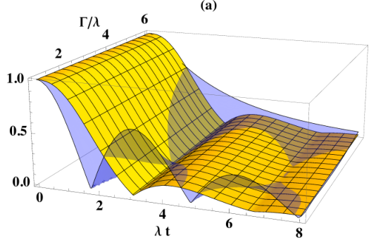
, considering a dephasing map $D(t)=\cos(\lambda t)$. In this case the dynamics given by $\mathcal{F}_{d}(t)$ alone never allows for a Markovian description. Here the rate $\lambda$ sets the natural time scale for this contribution to the dynamics, to be compared with the time scale $1/\Gamma$ given by the mean waiting time associated to the waiting time distribution $f(t)$. As it appears in Fig. 1(a), if $\Gamma/\lambda\gg 1$, so that subsequent events are very close in time, the contribution to NM due to $\mathcal{F}_{d}(t)$ is suppressed, since on a short enough time any time evolution map is Markovian.

As a further example we consider the dynamical map $\mathcal{F}_{+}(t)$, affecting both populations and coherences, that arises considering the interaction of a two-level system with a bosonic field in the vacuum state [1]. The map is characterized by the function $G(t)$, depending on the spectral density of the environment, and in matrix form reads

where $B(x)$ denotes the $4\times 4$ matrix with entry $x$ in the bottom left corner as the only non zero element. Exploiting Eq. (9) we can obtain the expression of the time evolution map [19]

where now $X(t)$ and $Y(t)$ take the expressions $g_{\pm}(t)=L^{\pm}_{f}\left[G\right](t)$, while $Z(t)$ corresponds to $h_{\pm}(t)=L^{\pm}_{f}[|G|^{2}](t)$. The function $W(t)$, determined by $f(t)$ and $|G(t)|^{2}$, does not affect the trace distance, since it corresponds to a fixed translation of the state [25]. A typical expression of $G(t)$ is given by

where $\tilde{\gamma}=\sqrt{\lambda^{2}-2\gamma\lambda}$, and has the interesting feature that for $\gamma/\lambda<1/2$ the map $\mathcal{F}_{+}(t)$ itself is Markovian, while for $\gamma/\lambda$ above this threshold one has NM [15]. The NM of the ensuing overall dynamics $\Lambda(t)$ is considered in Fig. 1(b), where we have plotted the modulus of the functions $g_{-}(t)$ and $h_{+}(t)$ for $G(t)$ as in Eq. (16). Again the growth of the modulus of any of these functions is a witness of NM. It appears indeed that for a wide range of parameters the dynamics is non-Markovian, yet the NM is actually the result of an interplay of the features of all the three elements determining the dynamics, namely $\mathcal{F}_{+}(t)$, $\mathcal{E}$ and $f(t)$. Indeed for values of the ratio $\gamma/\lambda$ such that $\mathcal{F}_{+}(t)$ itself is non-Markovian, the dynamics $\Lambda(t)$ might still be Markovian, if the ratio $\Gamma/\lambda$ of the time scales associated to $\mathcal{F}_{+}(t)$ and $f(t)$ is high enough. On the contrary, even a Markovian $\mathcal{F}_{+}(t)$ can give rise to a non-Markovian dynamics because of the action of the map $\mathcal{E}$ in between the continuous time evolutions, and of the distribution in time of these events.

We have obtained a large set of closed non-Markovian master equations starting from a piecewise dynamics described by a continuous time evolution interrupted by random jumps. The solution of these equations is warranted to be a CPT map. These master equations involve both a memory kernel and a inhomogeneous term. The basic ingredients in the construction are a collection of time dependent maps, together with a waiting time distribution describing the random occurrence of events characterized by a quantum channel. We have considered the connection of this result with the standard expression of quantum dynamical semigroups, as well as more recent examples of non-Markovian master equations obtained starting from microscopic models. In particular, we have certified the NM of the obtained time evolution by studying the behavior in time of the distinguishability between two different initial states, as quantified by the trace distance. Finally, the operational interpretation of the structure of these master equations paves the way for their use in concrete applications.

The author thanks A. Smirne for discussions and reading of the manuscript. Support from COST Action MP 1006 is gratefully acknowledged.

References

- [1] H.-P. Breuer and F. Petruccione, The Theory of Open Quantum Systems (Oxford University Press, Oxford, 2007)
- [2] U. Weiss, Quantum Dissipative Systems, 3rd edn. (World Scientific, Singapore, 2008)
- [3] A. S. Holevo, Statistical Structure of Quantum Theory (Springer, Berlin, 2001)
- [4] V. Gorini et al., J. Math. Phys. 17, 821 (1976)
- [5] G. Lindblad, Comm. Math. Phys. 48, 119 (1976)
- [6] S. M. Barnett and S. Stenholm, Phys. Rev. A 64, 033808 (2001)
- [7] A. A. Budini, Phys. Rev. A 69, 042107 (2004)
- [8] H.-P. Breuer and B. Vacchini, Phys. Rev. Lett. 101, 140402 (2008)
- [9] H.-P. Breuer and B. Vacchini, Phys. Rev. E 79, 041147 (2009)
- [10] R. Karplus and J. Schwinger, Phys. Rev. 73, 1020 (1973)
- [11] A. Rivas et al., Phys. Rev. Lett. 105, 050403 (2010)
- [12] D. Chruscinski and A. Kossakowski, e-print arXiv:1012:8079v1 (2012)
- [13] H.-P. Breuer et al., Phys. Rev. Lett. 103, 210401 (2009)
- [14] H.-P. Breuer, J. Phys. B 45, 154001 (2012)
- [15] E.-M. Laine et al., Phys. Rev. A 81, 062115 (2010)
- [16] L. Mazzola et al., Phys. Rev. A 81, 062120 (2010)
- [17] P. Haikka et al., Phys. Rev. A 83, 012112 (2011)
- [18] B. Vacchini et al., New J. Phys. 13, 093004 (2011)
- [19] See supplemental material for details
- [20] A. A. Budini, Phys. Rev. E 72, 056106 (2005)
- [21] B. Vacchini, J. Phys. B 45, 154007 (2012)
- [22] F. Ciccarello et al., e-print arXiv:1207:6554v1 (2012)
- [23] E. Andersson et al., J. Mod. Opt. 54, 1695 (2007)
- [24] A. Smirne and B. Vacchini, Phys. Rev. A 82, 022110 (2010)
- [25] S. Wissmann et al., Phys. Rev. A 86, 062108 (2012)
- [26] B. D. Hughes, Random walks and random environments. Vol. 1 (The Clarendon Press Oxford University Press, New York, 1995)