Database-assisted Distributed Spectrum SharingThanks: *Part of the results has been published at IEEE ICDCS 2012 [1].
Abstract
According to FCC’s ruling for white-space spectrum access, white-space devices are required to query a database to determine the spectrum availability. In this paper, we study the database-assisted distributed white-space access point (AP) network design. We first model the cooperative and non-cooperative channel selection problems among the APs as the system-wide throughput optimization and non-cooperative AP channel selection games, respectively, and design distributed AP channel selection algorithms that achieve system optimal point and Nash equilibrium, respectively. We then propose a state-based game formulation for the distributed AP association problem of the secondary users by taking the cost of mobility into account. We show that the state-based distributed AP association game has the finite improvement property, and design a distributed AP association algorithm that can converge to a state-based Nash equilibrium. Numerical results show that the algorithm is robust to the perturbation by secondary users’ dynamical leaving and entering the system.
I Introduction
The most recent FCC ruling requires that TV white-space devices must rely on a geo-location database to determine the spectrum availability [2]. In such a database-assisted architecture, the incumbents (primary licensed holders of TV spectrum) provide the database with the up-to-date information including TV tower transmission parameters and TV receiver protection requirements. Based on this information, the database will be able to tell a white-space device (secondary users (SUs) of TV spectrum) vacant TV channels at a particular location, given the white-space device’s transmission parameters such as the transmission power.
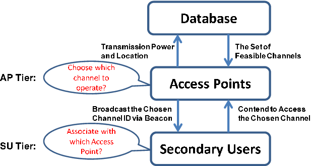
Although the database-assisted approach obviates the need of spectrum sensing, the task of developing a comprehensive and reliable database-assisted white-space network system remains challenging [3]. Motivated by the successful deployments of Wi-Fi over the unlicensed ISM bands, in this paper we consider an infrastructure-based white-space network (see Figure 1 for an illustration), where there are multiple secondary access points (APs) operating on white spaces. Such an infrastructure-based architecture has been adopted in IEEE 802.22 standard [4] and Microsoft Redmond campus white-space networking experiment [3]. More specifically, each AP first sends the required information such as its location and the transmission power to the database via wire-line connections. The database then feeds back the set of vacant TV channels at the location of each AP. Afterwards, an AP chooses one feasible channel to serve the secondary users (i.e., unlicensed white-space user devices) within its transmission range.
The key challenges for such an infrastructure-based white-space network design are twofold (see Figure 2 for an illustration). First, in the AP tier, each AP must choose a proper vacant channel to operate in order to avoid severe interference with other APs. Second, in the SU tier, when an AP is overloaded, a secondary user can improve its throughput by moving to and associating with another AP with less contending users. Each secondary user hence needs to decide which AP to associate with.

| Problem | Cooperative AP Channel Selection | Non-Cooperative AP Channel Selection | |
|---|---|---|---|
| AP Tier | Formulation | System-wide Throughput Optimization | Non-Cooperative AP Channel Selection Game |
| Algorithm | Cooperative AP Channel Selection Algorithm | Non-Cooperative AP Channel Selection Algorithm | |
| Problem | Distributed AP Association by SUs | ||
| SU Tier | Formulation | Distributed AP Association Game | |
| Algorithm | Distributed AP Association Algorithm | ||
In this paper, for the AP tier, we first consider the scenario that all the APs are owned by one network operator and hence the APs are cooperative. We formulate the cooperative AP channel selection problem as the system-wide throughput optimization problem. We then consider the scenario that the APs are owned by different network operators and the interest of APs is not aligned. We model the distributed channel selection problem among the APs as a non-cooperative AP channel selection game. For the SU tier, we propose a state-based game framework to model the distributed AP association problem of the secondary users by taking the cost of mobility into account. The main results and contributions of this paper are as follows (please refer to Table I for a summary):
- •
General formulation: We formulate the cooperative and non-cooperative channel selection problems among the APs as system-wide throughput optimization and non-cooperative AP channel selection game, respectively, based on the physical interference model [5]. We then propose a state-based game framework to formulate the distributed AP association problem of the secondary users and explicitly take the cost of mobility into account.
- •
Existence of equilibrium solution and finite improvement property: For the cooperative AP channel selection problem, the interest of APs is aligned and the system optimal solution that maximizes system-wide throughput always exists. For the non-cooperative AP channel selection game, we show that it is a potential game, and hence it has a Nash equilibrium and the finite improvement property. For the state-based distributed AP association game, we show that it also has a state-based Nash equilibrium and the finite improvement property.
- •
Distributed algorithms for achieving equilibrium: For the cooperative AP channel selection problem, we propose a cooperative channel selection algorithm that maximizes the system-wide throughput. For the non-cooperative AP channel selection game, we propose a non-cooperative AP channel selection algorithm that achieves a Nash equilibrium of the game. For the state-based distributed AP association game, we design a distributed AP association algorithm that converges to a state-based Nash equilibrium. Numerical results show that the algorithm is robust to the perturbation by secondary users’ dynamical leaving and entering the system.
The rest of the paper is organized as follows. We introduce the cooperative and non-cooperative AP channel selection problems, and propose the cooperative and non-cooperative AP channel selection algorithms in Sections II and III, respectively. We present the distributed AP association game and distributed AP association algorithm in Section IV. We illustrate the performance of the proposed mechanisms through numerical results in Section V, and finally introduce the related work and conclude in Sections VI and VII, respectively.
II Cooperative AP Channel Selection
II-A System Model
We first introduce the system model for the cooperative channel selection problem among the APs in the AP tier. Let denote the set of TV channels, and denote the bandwidth of each channel (e.g., MHz in the United States and MHz in the European Union). We consider a set of APs that operate on the white spaces. Each AP has a specified transmission power based on its coverage and primary user protection requirements.
Each AP can acquire the information of the vacant channels at its location from the geo-location database. We denote as the set of feasible channels of AP , as the channel chosen by AP 11 1 Following the conventions in IEEE 802.22 standard [4] and Microsoft Redmond campus white-space networking experiment [3], we consider the case that each AP can select one channel to operate on. The case that each AP can select multiple channels to operate on will be considered in a future work., and as the channel selection profile of all APs. Then the worse-case down-link throughput (i.e., the throughput at the boundary of the coverage area) of AP can be computed according to the physical interference model [5] as
| (1) |
where is the path loss factor, denotes the radius of the coverage area of AP , and denotes the distance between AP and the benchmark location at the boundary of the coverage area of AP . Furthermore, denotes the background noise power including the interference from incumbent users on the channel , and denotes the accumulated interference from other APs that choose the same channel . Note that we assume that all APs only try to maximize the worse-case throughputs by proper channel selections, which do not depend on the number of its associated users. However, the secondary users can increase their data rates by moving to and associating with a less congested AP (see Section IV for detailed discussions). Note that our model also applies to the up-link case if the secondary users within an AP transmit with roughly the same power level.
II-B Cooperative AP Channel Selection Algorithm
We first consider the case that all the APs try to maximize the system-wide throughput cooperatively. Such a cooperation is feasible when all the APs are owned by the same network operator. For example, the APs that are deployed in a university campus can coordinate to maximize the entire campus network throughput. Formally, the APs need to collectively determine the optimal channel selection profile such that the system-wide throughput is maximized, i.e.,
| (2) |
The problem (2) is a combinatorial optimization problem of finding the optimal channel selection profile over the discrete solution space . In general, such a problem is very challenging to solve exactly especially when the size of network is large (i.e., the solution space is large).
We next propose a cooperative channel selection algorithm that can approach the optimal system-wide throughput approximatively. To proceed, we first write the problem (2) into the following equivalent problem:
| (3) |
where is the probability that channel selection profile is adopted. Obviously, the optimal solution to problem (3) is to choose the optimal channel selection profile with probability one. It is known from [6] that problem (3) can be approximated by the following convex optimization problem:
| (4) |
where is the parameter that controls the approximation ratio. We see that when , the problem (4) becomes exactly the same as problem (3). That is, when the optimal point that maximizes the system throughput will be selected with probability one. A nice property of such an approximation in (4) is that we can obtain the close-form solution, which enables the distributed algorithm design later. More specifically, by the KKT condition [7], we can derive the optimal solution to problem (4) as
| (5) |

Similarly to the spatial adaptive play in [8] and Gibbs sampling in [9], we then design a cooperative AP channel selection algorithm by carefully coordinating APs’ asynchronous channel selection updates to form a discrete-time Markov chain (with the system state as the channel selection profile of all APs). As long as the Markov chain converges to the stationary distribution as given in (5), we can approach the optimal channel selection profile that maximizes the system-wide throughput by setting a large enough parameter . The details of the algorithm are given in Algorithm 1. Here APs’ asynchronous channel selection updates are scheduled by the database. In each iteration, one AP will be randomly chosen to update its channel selection. In this case, the direct transitions between two system states and are feasible if these two system states differ by one and only one AP channel selection. As an example, the system state transition diagram of the cooperative AP channel selection Markov chain by two APs is shown in Figure 3. We also denote the set of system states that can be transited directly from the state as , where denotes the size of a set.
Since each AP will be selected to update with a probability of and the selected AP will randomly choose a channel with a probability proportional to , then if , the probability that the Markov chain transits from state to is given as
| (6) |
Otherwise, we have . We show in Theorem 1 that the cooperative AP channel selection Markov chain is time reversible. Time reversibility means that when tracing the Markov chain backwards, the stochastic behavior of the reverse Markov chain remains the same. A nice property of a time reversible Markov chain is that it always admits a unique stationary distribution, which guarantees the convergence of the cooperative AP channel selection algorithm.
Theorem 1.
The cooperative AP channel selection algorithm induces a time-reversible Markov chain with the unique stationary distribution as given in (5).
Proof.
As mentioned, the system state of the cooperative AP channel selection Markov chain is defined as the channel selection profile of all APs. Since it is possible to get from any state to any other state within finite steps of transition, the AP channel selection Markov chain is hence irreducible and has a stationary distribution.
We then show that the Markov chain is time reversible by showing that the distribution in (5) satisfies the following detailed balance equations:
| (7) |
To see this, we consider the following two cases:
1) If , we have and the equation (7) holds.
According to Theorem 1, we can approach the system optimal point that maximizes the system-wide throughput by setting in the cooperative AP channel selection algorithm. However, in practice we can only implement a finite value of such that does not exceed the range of the largest predefined real number on a computer. Let be the expected potential by Algorithm 1 and be the global optimal potential. We show in Theorem 2 that, when a large eough is adopted, the performance gap between and is very small.
Theorem 2.
For the cooperative AP channel selection algorithm, we have that
where denotes the number of feasilbe channel selection profiles of all APs.
Proof.
We then analyze the computational complexity of the algorithm. In each iteration, one AP will be chosen for the channel selection update. Line involves the summation of the throughputs of APs for channels. Since , this step has the complexity of . Line involves at most summation and division operations and hence has a complexity of . Line has a complexity of . Suppose that it takes iterations for the algorithm to converge. Then total computational complexity of the algorithm is . Similarly, the space complexity of the algorithm is .
III Non-cooperative AP Channel Selection
We next consider the case that the APs are owned by different network operators. Unlike the previous case where the interest of the APs is aligned in the cooperative channel selection, here each AP is generally selfish and only concerns about its own throughput maximization. Formally, given other APs’ channel selections , the problem faced by an AP is to choose a proper channel to maximize its own throughput, i.e.,
The non-cooperative nature of the channel selection problem naturally leads to a formulation based on game theory, such that each AP can self organize into a mutually acceptable channel selection (Nash equilibrium) with
III-A Non-Cooperative AP Channel Selection Game
We now formulate the non-cooperative channel selection problem as a strategic game , where is the set of APs, is the set of strategies for AP , and is the payoff function of AP . We refer this as the non-cooperative AP channel selection game in the sequel.
We can show that it is a potential game, which is defined as
Definition 1 (Potential Game [10]).
A game is called a potential game if it admits a potential function such that for every and ,
where is the sign function defined as
Definition 2 (Better Response Update [10]).
The event where a player changes to an action from the action is a better response update if and only if .
An appealing property of the potential game is that it admits the finite improvement property, such that any asynchronous better response update process (i.e., no more than one player updates the strategy at any given time) must be finite and leads to a Nash equilibrium [10].
To show that the non-cooperative AP channel selection game is a potential game, we now consider a closely related game , where the new payoff functions are
| (9) |
Obviously, the utility function can be obtained from the utility function by the following monotone transformation
| (10) |
Due to the property of monotone transformation, we have
Lemma 1.
If the modified game is a potential game, then the original non-cooperative AP channel selection game is also a potential game with the same potential function.
Proof.
Since is a monotonically strictly increasing function, we have that
If the modified game is a potential game with a potential function such that
then we must also have that
which completes the proof. ∎
For the modified game , we show in Theorem 3 that it is a potential game with the following potential function
| (11) |
where if , and otherwise.
Theorem 3.
The modified game is a potential game with the potential function as given in (11).
Proof.
Suppose that an AP changes its channel to such that the strategy profile changes from to . We have that
Since , we thus have that
which completes the proof. ∎
Theorem 4.
The non-cooperative AP channel selection game is a potential game, which has a Nash equilibrium and the finite improvement property.
The result in Theorem 4 implies that any asynchronous better response update is guaranteed to reach a Nash equilibrium within a finite number of iterations. This motivates the algorithm design in Section III-B. Interestingly, according to the property of potential game, any channel selection profile that maximizes the potential function is a Nash equilibrium [10]. According to (11), the profile is also an efficient system-wide solution, since maximizing the potential function is equivalent to minimizing the total weighted interferences (with a weight of ) among all the APs.
III-B Non-Cooperative AP Channel Selection Algorithm
The purpose of designing this algorithm is to allow APs to select their channels in a distributed manner to achieve a mutually acceptable resource allocation, i.e., an Nash equilibrium. The key idea is to let APs asynchronously improve their channel selections according to the finite improvement property.
We assume that when an AP queries the geo-location database, the database will assign it with a unique ID indexed as . For initialization, we let each AP select the channel that has the smallest channel ID index among its feasible channels , i.e., . Then based on the initialized channel selection profile , each AP in turn (according to the assigned IDs) carries out the best response update, i.e., select a channel that maximizes its own throughput as
| (12) |
given the channel selections of the updated APs, and the channel selections of remaining APs that are not updated at the current stage . Such update procedure continues until a Nash equilibrium is reached. Since the best response update is also a better response update, according to the finite improvement property, such asynchronous best response updates must achieve a Nash equilibrium within finite number of iterations. We summarize the non-cooperative AP channel selection algorithm in Algorithm 2. We then consider the computational complexity of the algorithm. Lines to involves maximization operations and each maximization operation can be achieved by sorting over at most values. This step typically has a complexity of . Line has the complexity of . Suppose that it takes iterations for the algorithm to converge. Then total computational complexity of the algorithm is . Similarly, the space complexity of the algorithm is .
The Algorithm 2 requires all APs to truthfully communicate with each other about their channel selections. When such a requirement is not feasible, each AP can independently implement Algorithm 2 by acquiring the assigned IDs, available channels, and transmission powers of other APs from the database. Note that such an off-line implementation is incentive compatible, since given other APs adhere to the algorithm and the update order is fixed, no AP has an incentive to deviate unilaterally from the algorithm (due to the deterministic Nash equilibrium output).
III-C Price of Anarchy
We now study the efficiency of Nash equilibria of the non-cooperative AP channel selection Game. Following the definition of price of anarchy (PoA) in game theory [11], we will quantify the efficiency ratio of the worst-case Nash equilibrium over the optimal solution by the cooperative AP channel selection. Let be the set of Nash equilibria of the game. Then the PoA is defined as
which is always not greater than . A larger PoA implies that the set of Nash equilibrium is more efficient (in the worst-case sense when comparing with the system optimal solution). Let and . We can first show that
Lemma 2.
For the non-cooperative AP channel selection game, the throughput of an AP at a Nash equilibrium is no less than where is the number of vacant channels for AP .
Proof.
We will prove the result by contradiction. Suppose that an AP at a Nash equilibrium has a throughput less than . From the throughput function in (1), we must have that
| (13) |
According to the definition of Nash equilibrium (no AP can improve by changing channel unilaterally), we also have that
| (14) |
which implies that
| (15) | |||||
According to (13) and (15), we now reach a contradiction that
This proves the result. ∎
Lemma 2 implies that at a Nash equilibrium each AP will receive an interference level that is not greater than the maximum possible interference level (i.e., ) divided by the number of its available channels. That is, if more channels are available then the performance of Nash equilibria can be improved. According to Lemma 2, we know that
Corollary 1.
The PoA of the non-cooperative AP channel selection game is lower bounded by
Proof.
The PoA characterizes the worst-case performance of Nash equilibria. Numerical results in Section VII demonstrate that the convergent Nash equilibrium of the proposed algorithm in Section III-B is often more efficient than what the PoA indicates and the performance loss is less than , compared with the optimal solution by the cooperative AP channel selection.
IV Distributed AP Association By Mobile Secondary Users
We now consider the distributed AP association problem among a set of mobile secondary users in the SU tier. Let be the number of users that associate with AP , which satisfies that . We assume that the APs’ cooperative/non-cooperative channel selections in the AP tier and the users’ AP associations in the SU tier are decoupled, i.e., APs only interested in guaranteeing their throughputs by proper channel selections and users can improve their data rates by proper AP associations. The load-aware AP channel selection will be considered in a future work.
IV-A Channel Contention Within an AP
We first consider the channel contention when multiple secondary users associate with the same AP. Here we adopt a random backoff mechanism to resolve the channel contention. More specifically, the time is slotted (see Figure 4), with a contention stage being divided into mini-slots.22 2 For the ease of exposition, we assume that the contention backoff size is fixed. This corresponds to an equilibrium model for the case that the backoff size can be dynamically tuned according to the 802.11 distributed coordination function [12]. Also, we can enhance the performance of the backoff mechanism by determining optimal fixed contention backoff size according to the method in [13]. Each secondary user executes the following two steps:
- 1.
Count down according to a randomly and uniformly chosen integral backoff time (number of mini-slots) between and .
- 2.
Once the timer expires, monitor the channel and exchange RTS/CTS messages with the AP in order to grab the channel if the channel is clear (i.e., no ongoing transmission). Note that if multiple users choose the same backoff mini-slot, a collision will occur with RTS/CTS transmissions and no users can grab the channel. Once the RTS/CTS message exchange goes through, then the AP starts to transmit the data packets to the user.
Since users contend for the channel in AP , the probability that a user (out of these users) grabs the channel successfully is
| (16) |
which is a decreasing function of the total number of contending users . Then the average data rate of a secondary user associating with AP is given as
| (17) |
where is the throughput at the boundary of the coverage area of AP at the equilibrium channel selections by cooperative/non-cooperative AP channel selection algorithms, and is the transmission gain of user . Here the transmission gain is used to model user specific throughputs due to their heterogeneous channel conditions. For example, a user enjoys a better channel condition than all other users if it is the closest to the AP.

IV-B Distributed AP Association Game
Due to the channel contention within an AP , the average data rate of a secondary user decreases with the total number of contending users . To improve the data rate , the secondary user can choose to move to another AP with less users. However, in practices people may not prefer long distance movements (just for the sake of obtaining better communication experiences), which motivates us to take the cost of mobility into account. By defining the current location profile of all secondary users as a system state, we next formulate the distributed AP association problem as a state-based game [14] as follows:
- •
Player : a secondary user from the set .
- •
Strategy : choose an AP to associate with. We denote the strategy profile of all users as .
- •
State : the current locations (i.e., the associated APs) of all secondary users, where denote the location of user .
- •
State Transition : in general the new state is determined by the strategies of all secondary users and the original state , where denotes the state transition function. For our problem, we have that , i.e., the new locations just depend on secondary users’ AP choices and independent of the original system state.
- •
Payoff : secondary user ’s utility obtained from the strategy profile in state . To take the cost of mobility into account, we define
(18) where is the number of contending users associated with AP under strategy profile , is the factor representing the weight of mobility cost in user ’s decision, and is the distance of moving to AP from AP ( if ). Note that the distance measure here can represent more general preference functions and can also be asymmetric. For example, we can define that if is a popular shopping mall where uses like to stay. The physical meaning of (18) is to balance the average data rate that a user can obtain from moving to a new AP with the mobility cost by moving from its current associated AP .
Since the state-based game is a generalized game theoretic framework (by regarding the classical strategic game as a state-based game with a constant state), we need an updated equilibrium concept. Here we follow the recent results in [14] and introduce the state-based Nash equilibrium. To proceed, we first define the set of reachable states starting from a strategy state pair as
| (19) |
We then extend the definition of Nash equilibrium to the state-based game setting as follows.
Definition 3 (State-based Nash Equilibrium [14]).
A strategy state pair
is a state-based Nash equilibrium if
1) the state is reachable from , i.e.,
.
2) for every player and every state ,
we have
| (20) |
The physical meaning of the state-based Nash equilibrium is that the state is recurrent and the strategy profile is the best response no matter how the game state evolves after-wards. In principle, the state-based game is a special case of the stochastic game, which is difficult to tackle. However, we are able to solve the distributed AP association game by exploiting its inherent structure property. A key observation is that, similarly to the classical potential game, the state-based distributed AP association game also admits a state-based potential function as
| (21) |
For the state-based potential function , we have
Lemma 3.
For the state-based distributed AP association game, if a player performs a better response update in a given state with
we then have that
Proof.
Similarly to the classical potential game, we can also define the finite improvement property for the state-based game. Let be the state of the game in the -th update, and be the strategy profile of all players in -th update. According to the state transition, we have . A path of the state-based game is a sequence such that for every there exists a unique player, say player , such that for some strategy . is an improvement path if for all we have , where is the unique deviator at the -th update. From the properties of the state-based potential function , we first show that every improvement path is finite.
Theorem 5.
For the state-based distributed AP association game, every improvement path is finite.
Proof.
For any improvement path , we have
where , , and so on. From Lemma 3, we know that
which is increasing along the improvement path. Since , then the improvement path must be finite. ∎
Similarly to the classical potential game, we further show that any asynchronous better response update process also leads to a state-based Nash equilibrium.
Theorem 6.
For the state-based distributed AP association game, any asynchronous better response update process leads to a state-based Nash equilibrium with .
Proof.
Suppose that an asynchronous better response update process terminates at the point . In this case, we must have , otherwise the improvement path does not terminate at point . At point , we must also have that and , otherwise the potential function can be improved and thus the improvement path does not terminate here. Thus, we have and , which satisfies the conditions in Definition 3. ∎
Since , Theorem 6 implies that the asynchronous better response update process leads to the state-based Nash equilibrium (), i.e., the equilibrium that all users are satisfied with the current AP associations and have no incentive to move anymore.
IV-C Distributed AP Association Algorithm
We next design a distributed AP association algorithm based on the finite improvement property shown in Theorem 5, which allows secondary users to select their associated APs in a distributed manner and achieve mutually acceptable AP associations, i.e., a state-based Nash equilibrium.
The key idea is to let secondary users asynchronously improve their AP selections. Unlike the non-cooperative AP channel selection update with the fixed order enforced by the geo-location database, the distributed AP association algorithm can not be deterministic. This is because that, as secondary users dynamically enter and leave the network, a deterministic distributed AP association algorithm according to the fixed strategy update order is not robust. Hence we will design a randomized algorithm by letting each secondary user countdown according to a timer value that follows the exponential distribution with a mean equal to . Since the exponential distribution has support over and its probability density function is continuous, the probability that more than one users generate the same timer value and update their strategies simultaneously equals zero.33 3 The timer in practice is always finite, and the collision probability is not exactly zero. However, as long as the collision probability is very small, the following analysis is a very good approximation of the reality. When a user activates its strategy update at time , the user can computes its best response strategy as
| (24) |
which requires the information of user distribution at time , the throughput , and geo-locations of all the APs. We then consider the computational complexity of the algorithm. For each iteration of each user, Lines to only involve random value generation and subduction operation for count-down, and hence have a complexity of . Line involves information inquiry from APs and hence has a complexity of . Line computes the best response strategy, which can be achieved by sorting at most values and typically has a complexity of . Suppose that it takes iterations for the algorithm to converge. Then total computational complexity of users is . Similarly, we can show that the space complexity is .
To facilitate the best response update, we propose to setup a social database (accessible by all secondary users), wherein each AP reports its channel throughput and geo-location, and each secondary user posts and shares its AP association with other users in the manner like Twitter once it updates. Based on the information from the social database, a secondary user can first figure out the user distribution as
| (25) |
where if user associates with AP , and otherwise. Based on the user distribution, the secondary user can then compute the corresponding best response strategy according to (24).
The success of social database requires that each user is willing to share the information of its AP association. When this is not feasible, each AP can estimate its associated user population locally. Let denote the probability that no user among associated with the same AP grabs the channel in a time slot . This can be computed as , where is given in (16). In a time slot , AP can observe the information , i.e., whether the channel is used by any users or not. Then over a long period that consists of time slots, AP can observe the outcome and estimate by the sample-average. Since is independently and identically distributed according to the probability , according to the law of large numbers, the estimation will be accurate when the observation period length is large enough. This is feasible in practices since user’s mobility decision is often carried out at a large time scale (say every few minutes), compared with the time scale of a time slot (say microseconds in the standard 802.11 system). Then AP can obtain the number of its associated users by solving that , and report it in the social database.
We summarize the distributed AP association algorithm in Algorithm 3. According to Theorem 6, such asynchronous best response update process must reach a state-based Nash equilibrium. Numerical results show that the algorithm is also robust to the dynamics of secondary users’ leaving and entering the system.
V Simulation Results
In this part, we investigate the proposed AP channel selection and AP association algorithms by simulations.
V-A Cooperative AP Channel Selection
We first implement the cooperative AP channel selection algorithm in Section II. We consider a white-space wireless system consisting of channels and APs, which are scattered across a square area of a length of m (see Figure 5). The bandwidth of each channel is MHz, the noise power is dBm, and the path loss factor . Each AP operates with a specific transmission power and has a different set of vacant channels by consulting the geo-location database (please refer to Figure 5 for the details of these parameters). We set that the distance between AP and its associated boundary secondary user is m.
We implement the cooperative channel selection algorithm with the parameter , and , respectively44 4 Note that the system throughput is a large number in the Mbps unit and a small is adopted in the simulation. Otherwise, would exceed the range of the largest predefined real number on a personal computer. However, if we measure the system throughput in the Gbps unit, the parameter is large and becomes , and , respectively.. We show the dynamics of the time average throughputs of all the APs in Figure 6 when . It demonstrates the convergence of the cooperative channel selection algorithm. From Figure 7, we see that the performance of the algorithm improves as the increases, and the convergence time also increases accordingly. When , the performance loss of the cooperative channel selection algorithm is less than , compared with the centralized optimal solution, i.e., . Moreover, the algorithm achieves more than performance gain over the random channel selection scheme wherein the APs choose channels purely randomly.


V-B Non-Cooperative AP Channel Selection
We then implement the non-cooperative channel selection algorithm in Section III. We show the dynamics of the throughputs of all the APs in Figure 8. We see that the algorithm converges to an equilibrium in less iterations. To verify that the equilibrium is a Nash equilibrium, we show the dynamics of the potential function in Figure 9. We see that the algorithm can lead the potential function to a maximum point, which is a Nash equilibrium according to the property of potential game. At the equilibrium , APs achieve the throughputs of Mbps, respectively, and no AP has the incentive to deviate its channel selection unilaterally. Compared with cooperative AP channel selection algorithm, the performance loss of the non-cooperative channel selection algorithm is less than . Such a performance loss is due to the selfishness of APs in the non-cooperative environment. However, the convergence time of non-cooperative AP channel selection algorithm is much shorter. This is because that in order to achieve the system optimal solution, the cooperative algorithm needs more time to randomly explore the whole set of feasible channel selections. While the non-cooperative channel selection algorithm achieves the Nash equilibrium by focusing on the subset of channel selections satisfying the finite improvement property.
We then further implement simulations with APs being randomly scattered over the square area in Figure 5, respectively. The number of TV channels and channels out of these channels will be randomly chosen as the set of vacant channels for each AP . We implement both non-cooperative and cooperative AP channel selection algorithms. The results are shown in Figure 12. We see that when the number of APs is small (e.g., ), the non-cooperative channel selection achieves the same performance as the cooperative case. This is due to the abundance of the spectrum resources. We also observe that the performance of the non-cooperative channel selection algorithm is less than in all cases. This demonstrates the efficiency of the non-cooperative channel selection.


V-C Distributed AP Association
We next implement the distributed AP association algorithm in Section IV. We consider mobile secondary users who can move around and try to find a proper AP to associate with. Within an AP , the worse-case throughput of AP is computed according to the Nash equilibrium in Section V-B. For the channel contention by multiple secondary users, we set the number of backoff mini-slots .
We first show in Figure 10 the dynamics of the distributed AP association algorithm with the random initial APs selections, users’ transmission gains being randomly selected from the set , and the mobility cost factor Mbps/m. We see that the algorithm converges to an equilibrium in less iterations. We also show the the dynamics of the state-based potential function in Figure 11. We see that the equilibrium is a state-based Nash equilibrium, since the algorithm leads the state-based potential function to a maximum point.

To investigate the impact of the cost factor , we assume that all the users are initially associated with AP with the same transmission gains and they change AP associations according to the distributed AP association algorithm with four different settings in Figure 13. In each setting, all users have the same cost factor . As the mobility cost increases, we see that less secondary users are willing to move away from their initial APs. When the cost , the secondary users are scattered across all APs since there is no cost due to mobility. When , only a small fraction of secondary users move away from the initial AP to the APs closeby, due to the high cost of mobility. In Figure 14, we further implement the algorithm with a mixture of two types of secondary users: high and low mobility cost factors. We see that users of low mobility cost will spread out to achieve better data rates, while most users of high mobility cost choose to stay in AP and suffer from severe congestion.
We next investigate the robustness of the distributed AP association algorithm. We consider mobile secondary users with the cost factor randomly generated from a uniform distribution in . At iteration and , we let users leave the system and new users enter the system, respectively. The results in Figures 15 and 16 show that the algorithm can quickly converge to a state-based Nash equilibrium after the perturbations occur. This verifies that the distributed AP association algorithm is robust to the dynamics of secondary users’ leaving and entering the system.


VI Related Work
Most research efforts in database-assisted white-space systems are devoted to the design of geo-location service. Gurney et al. in [15] calculated the spectrum availability based on the transmission power of the white-space devices. Karimi in [16] presented a method to derive location-specific maximum permitted emission levels for white space devices. Murty et al. in [3] proposed a framework to determine the vacant spectrum by using propagation model and terrain data. Nekovee in [17] studied the white-space availability and frequency composition in UK.
For the white-space networking system design, many existing works focus on the experimental testbed implementation. Bahl et al. in [18] designed a single white-space AP system. Murty et al. in [3] addressed the client bootstrapping and mobility handling issues in white-space AP networks. Feng et al. in [19] considered the OFDM-based AP white-space network system design. Deb et al. in [20] presented a centralized white-space spectrum allocation algorithm. In this paper, we propose a theoretic framework based on game theory for distributed resource allocation in white-space AP networks.
The game theory has been used to study wireless resource allocation problems in non-white-space infrastructure-based networks. Song et al. in [21] modeled the distributed channel allocation in mesh networks as a non-cooperative game, where each cell tries to minimize the interference received from other cells. Southwell et al. in [22] modeled the distributed channel selection problem with switching cost as a network congestion game. Chen and Huang in [23] proposed a spatial spectrum access game framework for distributed spectrum sharing with spatial reuse. Wang et al. in [24] proposed an auction approach for incentive-compatible spectrum resource allocation. Most previous works studied the competitive channel selection based on the protocol interference model where two users can interfere with each other if they are linked by an interference edge on the interference graph. In this paper, we explore the competitive channel selections based on the physical interference model, which is not well studied in the literature. The most relevant work is [9], where Kauffmann et al. considered to minimize the total interferences received by all the APs by designating each AP a specific utility function to be optimized locally. In our paper, we consider the case that each AP is fully rational and tries to maximize its own throughput.
For the AP association problem, Gajić et al. in [25] and Duan et. al in [26] studied the pricing mechanisms to achieve efficient wireless service provider association solutions. Bejerano et al. in [27] address the load imbalance problem through the association control. Hong et al. in [28] investigated distributed AP association game with power control, by assuming that the chosen channels among APs are non-overlapping. These previous results focus on the case that users are stationary, and can associate with any AP. When users are mobile, Mittal et al. in [29] studied the distributed access point selection game by assuming that users are homogeneous with the same cost of mobility. Here we propose a state-based game framework to formulate the more general case that users have heterogeneous cost of mobility.
VII Conclusion
In this paper, we consider the database-assisted white-space AP network design. We address the cooperative and non-cooperative channel selection problems among the APs and the distributed AP association problem of the secondary users. We propose the cooperative and non-cooperative AP channel selection algorithms and a distributed AP association algorithm, all of which that converge to the corresponding equilibrium globally. Numerical results show that the proposed algorithms are efficient, and are also robust to the perturbation by secondary users’ dynamical leaving and entering the system.
For the future work, we are going to generalize the results to the mixture case that consists of both cooperative and non-cooperative APs. Multiple APs that belong to one network operator are cooperative with each other, but they may not cooperate with other APs that belong to a different network operator. It will be interesting to study the existence of Nash equilibrium and design distributed algorithms to achieve the equilibrium.
Although the distributed AP association algorithm can achieve the state-based Nash equilibrium wherein all users are satisfied given their mobility cost factors, the loads among different APs can be quite imbalanced when the mobility cost is high as demonstrated in the numerical results. Thus, how to design an incentive compatible mechanism such as pricing to achieve load balance among the APs with mobile secondary users will be very interesting and challenging.
References
- [1] X. Chen and J. Huang, “Game theoretic analysis of distributed spectrum sharing with database,” in the 32nd International Conference on Distributed Computing Systems (ICDCS), 2012. [Online]. Available: http://ncel.ie.cuhk.edu.hk/sites/default/files/ICDCS2012.pdf
- [2] FCC, “Second memorandum opinion and order,” September 23, 2010. [Online]. Available: http://transition.fcc.gov/Daily_Releases/Daily_Business/2010/db0923/FCC-10-174A1.pdf
- [3] R. Murty, R. Chandra, T. Moscibroda, and P. Bahl, “Senseless: A database-driven white spaces network,” in IEEE Symposia on New Frontiers in Dynamic Spectrum Access Netoworks (DySpan), 2011.
- [4] IEEE 802.22 Working Group, “IEEE 802.22 draftv3.0,” 2011. [Online]. Available: http://www.ieee802.org/22/
- [5] P. Gupta and P. R. Kumar, “The capacity of wireless networks,” IEEE Transactions on Information Theory, vol. 46, no. 2, pp. 388–404, 2000.
- [6] M. Chen, S. Liew, Z. Shao, and C. Kai, “Markov approximation for combinatorial network optimization,” in INFOCOM, 2010 Proceedings IEEE. IEEE, 2010, pp. 1–9.
- [7] S. Boyd and L. Vandenberghe, Convex optimization. Cambridge university press, 2004.
- [8] H. Young, Individual strategy and social structure: An evolutionary theory of institutions. Princeton University Press, 2001.
- [9] B. Kauffmann, F. Baccelli, A. Chaintreau, V. Mhatre, K. Papagiannaki, and C. Diot, “Measurement-based self organization of interfering 802.11 wireless access networks,” in INFOCOM 2007. 26th IEEE International Conference on Computer Communications. IEEE. IEEE, 2007, pp. 1451–1459.
- [10] D. Monderer and L. S. Shapley, “Potential games,” Games and Economic Behavior, vol. 14, pp. 124–143, 1996.
- [11] T. Roughgarden and E. Tardos, “Introduction to the inefficiency of equilibria,” Algorithmic Game Theory, vol. 17, pp. 443–459, 2007.
- [12] G. Bianchi, “Performance analysis of the IEEE 802.11 distributed coordination function,” IEEE Journal on Selected Areas in Communications, vol. 18, no. 3, pp. 535–547, 2000.
- [13] E. Kriminger and H. Latchman, “Markov chain model of homeplug CSMA MAC for determining optimal fixed contention window size,” in IEEE International Symposium on Power Line Communications and Its Applications (ISPLC), 2011.
- [14] N. Li and J. R. Marden, “Designing games to handle coupled constraints,” in IEEE CDC, 2010, pp. 250–255.
- [15] D. Gurney, G. Buchwald, L. Ecklund, S. Kuffner, and J. Grosspietsch, “Geo-location database techniques for incumbent protection in the tv white space,” in IEEE Symposia on New Frontiers in Dynamic Spectrum Access Netoworks (DySpan), 2008.
- [16] H. R. Karimi, “Geolocation databases for white space devices in the uhf tv bands: Specification of maximum permitted emission levels,” in IEEE Symposia on New Frontiers in Dynamic Spectrum Access Netoworks (DySpan), 2011.
- [17] M. Nekovee, “Quantifying the availability of tv white spaces for cognitive radio operation in the uk,” Tech. Rep., 2009. [Online]. Available: http://arxiv.org/abs/0906.3394v1
- [18] P. Bahl, R. Chandra, T. Moscibroda, R. Murty, and M. Welsh, “White space networking with wi-fi like connectivity,” in SIGCOMM, 2009, pp. 27–38.
- [19] X. Feng, J. Zhang, and Q. Zhang, “Database-assisted multi-ap network on tv white spaces: Architecture, spectrum allocation and ap discovery,” in IEEE Symposia on New Frontiers in Dynamic Spectrum Access Netoworks (DySpan), 2011.
- [20] S. Deb, V. Srinivasan, and R. Maheshwari, “Dynamic spectrum access in DTV whitespaces: design rules, architecture and algorithms,” in MOBICOM, 2009, pp. 1–12.
- [21] Y. Song, C. Zhang, and Y. Fang, “Joint channel and power allocationin wireless mesh networks: A game theoretical perspective,” IEEE Journal on Selected Areas in Communications, vol. 26, no. 7, pp. 1149–1159, 2008.
- [22] R. Southwell, J. Huang, and X. Liu, “Spectrum mobility games,” in IEEE INFOCOM, 2012.
- [23] X. Chen and J. Huang, “Spatial spectrum access game: Nash equilibria and distributed learning,” in ACM International Symposium on Mobile Ad Hoc Networking and Computing (MobiHoc), 2012.
- [24] X. Wang, Z. Li, P. Xu, Y. Xu, X. Gao, and H. Chen, “Spectrum sharing in cognitive radio networks¡ªan auction-based approach,” IEEE Transactions on Systems, Man, and Cybernetics, Part B: Cybernetics, vol. 40, no. 3, pp. 587–596, 2010.
- [25] V. Gajic, J. Huangy, and B. Rimoldi, “Competition of wireless providers for atomic users: Equilibrium and social optimality,” in 47th annual Allerton conference on Communication, control, and computing, 2009.
- [26] L. Duan, J. Huang, and B. Shou, “Competition with dynamic spectrum leasing,” in IEEE Symposia on New Frontiers in Dynamic Spectrum Access Netoworks (DySpan), 2010.
- [27] Y. Bejerano, S. Han, and L. Li, “Fairness and load balancing in wireless lans using association control,” in Proceedings of the 10th annual international conference on Mobile computing and networking. ACM, 2004, pp. 315–329.
- [28] M. Hong, A. Garcia, and J. Barrera, “Joint distributed access point selection and power allocation in cognitive radio networks,” in INFOCOM, 2011, pp. 2516–2524.
- [29] K. Mittal, E. M. Belding, and S. Suri, “A game-theoretic analysis of wireless access point selection by mobile users,” Computer Communications, vol. 31, no. 10, pp. 2049–2062, 2008.