Multi-Level Monte Carlo approaches for numerical homogenization

Yalchin Efendiev ^†^†thanks: Department of Mathematics, Texas A & M University, College Station, TX 77845, USA Cornelia Kronsbein ^†^†thanks: Fraunhofer ITWM & University of Kaiserslautern, 67663 Kaiserslautern, Germany Frédéric Legoll ^†^†thanks: Laboratoire Navier, École des Ponts ParisTech, Université Paris-Est, 6 et 8 avenue Blaise Pascal, 77455 Marne-La-Vallée Cedex 2, France and INRIA Rocquencourt, MICMAC Team-Project, Domaine de Voluceau, B.P. 105, 78153 Le Chesnay Cedex, France

August 24, 2026

Abstract

Abstract. In this article, we study the application of Multi-Level Monte Carlo (MLMC) approaches to numerical random homogenization. Our objective is to compute the expectation of some functionals of the homogenized coefficients, or of the homogenized solutions. This is accomplished within MLMC by considering different levels of representative volumes (RVE), and, when it comes to homogenized solutions, different levels of coarse-grid meshes. Many inexpensive computations with the smallest RVE size and the largest coarse mesh are combined with fewer expensive computations performed on larger RVEs and smaller coarse meshes. We show that, by carefully selecting the number of realizations at each level, we can achieve a speed-up in the computations in comparison to a standard Monte Carlo method. Numerical results are presented both for one-dimensional and two-dimensional test-cases.

1 Introduction

Many multi-scale problems have uncertainties at the smallest scales, that are due to the incomplete knowledge one has of the microstructure. For example, when considering porous materials, the microstructure is often generated based on some limited statistical information. This can lead to large uncertainties in terms of microscale heterogeneities. These uncertainties at micro-scales need to be mapped onto the simulations on a coarse-grid, and this typically leads to considering large representative volumes (RVE) for these microstructures.

In practice, the upscaled quantities that are used at the macroscopic level are computed using the solution of some local problems posed on these microstructures. It is often needed to solve many such local problems (corresponding to many different random realizations, or snapshots, of the microstructure), each of which being expensive due to the presence of small scales. The resulting amount of computational work may thus be prohibitively expensive. In this article, our objective is to design a computational approach that allows for fast calculations of the coarse-scale quantities based on fewer realizations.

Our idea is to apply the Multi-Level Monte Carlo (MLMC) framework to multi-scale simulations. The MLMC approach was first introduced by Heinrich in [23] for finite- and infinite-dimensional integration. Later on, it was applied to stochastic ODEs by Giles (see [21, 20]). More recently, this approach has been used for PDEs with stochastic coefficients by several authors, see [4, 16, 1, 14, 27]. To compute an approximation of the expectation ${\mathbb{E}}(X)$ of some random variable $X$ , the MLMC approach consists in considering several random variables $X_{l}$ , at different levels $l$ , that approximate $X$ with various accuracies. The main idea is then to use different numbers of samples (i.e. independent realizations) at different levels. More precisely, many samples are used at the coarsest, less accurate level where the computation for each realization is inexpensive, while fewer samples are used at the finest, most accurate level that is expensive to compute. Combining the results of these computations by carefully selecting the number of realizations at each level can speed-up the computations in comparison to a standard Monte Carlo (MC) approach, where only one level (that of the quantity of interest itself) is considered. See Section 2.2 below for more details on the MLMC approach.

In the framework of numerical stochastic homogenization, local problems are solved on representative volumes (RVE), and apparent effective properties are next defined as averages of the solutions of these local problems over the RVEs. The computations on the RVEs are usually expensive, because large RVEs need to be considered to obtain effective properties with a reasonable accuracy. In the framework of MLMC approaches, our idea is to use RVEs of different sizes, and to consider many independent realizations of the smaller ones, for which the associated local problem is inexpensive to solve, and fewer realizations of the larger ones.

The convergence of the MLMC approach depends on the accuracy of the computations at each level. Assessing how this accuracy improves when more expensive computations are considered is critical to determine how to choose the number of realizations at each level. In our case, we thus have to determine how the accuracy of apparent effective properties depend on the RVE size. Such estimations are not easy to obtain, both from a theoretical and a practical viewpoint. In this work, we use the fact that, under some assumptions on the heterogeneous coefficients, it is known that the accuracy of the effective property approximation scales as $(\epsilon/\eta)^{\beta}$ for some $\beta>0$ , where $\eta$ is the RVE size and $\epsilon$ is the characteristic small lengthscale of the heterogeneities (see e.g. [3, 8, 9, 11, 17, 19, 22, 24, 28]).

When the MLMC approach is used to compute the expectation of some functionals of the homogenized solution (rather than the homogenized coefficient), we can use RVEs of different size to compute the homogenized coefficients, and also coarse grids with various size to solve the coarse scale equation. In addition to assessing the accuracy of the approximation of the effective properties in each RVE, we need to assess the accuracy when solving the coarse-scale equation. Standard FEM results are then useful.

An important remark is that MLMC approaches are interesting when effective properties are stochastic (otherwise, such approaches are as efficient as a standard MC approach). This situation appears in many applications, although homogenization theories for this case are less studied. Most homogenization theories are indeed developed for ergodic coefficients that vary over a single scale. In this case, the apparent homogenized quantities, when computed on infinitely large RVEs, are deterministic. In the sequel, we briefly discuss homogenization results when the homogenized coefficient is stochastic (even when infinitely large RVEs are considered), and we use these results in our MLMC approach to adequately select the number of realizations at each level (namely, for each RVE size and each coarse grid size).

Consider now the specific question of computing homogenized solutions with several grids of different size. For each of these grids, we first need to precompute the effective properties, say at each Gauss point of the macroscopic grid. Assume that these coarse grids are nested. Then, once the effective properties have been computed at the finest level (i.e. for the Gauss points of the finest grid), no additional precomputation is needed to compute effective properties for the coarser grids (since their Gauss points are a subset of the Gauss points of the finest grid). In this case, we propose to use a weighted MLMC approach, where we give different weights to each level, so as to optimize the accuracy at a given cost.

Our article is organized as follows. In Section 2, we briefly review theoretical homogenization results and describe in details the MLMC approach in a general context. In Section 3, we next describe how to apply the MLMC approach to compute an approximation of the homogenized coefficients, and assess the accuracy of the proposed approach. We next turn in Section 4 to the computation of the homogenized solutions, using either the MLMC or the weighted MLMC approaches. Numerical results are collected in Section 5. We consider the case of the effective coefficients in Section 5.2, and of the homogenized solutions in Section 5.3. In both cases, we show that the MLMC approach yields a significant speed-up in comparison to a standard MC approach.

2 Preliminaries

2.1 Numerical homogenization

In this section, we describe the numerical homogenization procedure we use. Consider the problem

-\text{div}(A_{\epsilon}(x,\omega)\nabla u_{\epsilon})=f\text{ in $D$},

(1)

where $D$ is an open bounded subset of ${\mathbb{R}}^{d}$ , $A_{\epsilon}(x,\omega)$ is a heterogeneous random field (with a small characteristic length scale $\epsilon$ ), $\omega$ designates a random realization and $f\in L^{2}(D)$ is a non-random function. We complement the problem (1) with some boundary conditions that we do not specify, such that its solution $u_{\epsilon}$ is well defined (for instance, $u_{\epsilon}=0$ on $\partial D$ almost surely). Furthermore, we assume that $A_{\epsilon}$ is uniformly bounded and coercive, in the sense that there exists two positive deterministic numbers $0<a_{\text{min}}\leq a_{\text{max}}$ such that, for any $\epsilon$ , any $\xi\in{\mathbb{R}}^{d}$ and any $1\leq i,j\leq d$ ,

a_{\text{min}}|\xi|^{2}\leq\xi^{T}A_{\epsilon}(x,\omega)\xi,\quad\left|\left[A_{\epsilon}(x,\omega)\right]_{ij}\right|\leq a_{\text{max}},

almost everywhere in $D$ and almost surely.

For almost all realizations $\omega$ , we consider a numerical homogenization procedure as follows. Given a representative volume centered at a macroscopic point $x$ with size $\eta$ ,

Y_{\eta}^{x}=\left(x-\frac{\eta}{2},x+\frac{\eta}{2}\right)^{d},

we solve, for any $1\leq i\leq d$ , the local problems

\text{div}(A_{\epsilon}(y,\omega)\nabla\chi_{i}(y,\omega))=0\text{ in $Y_{\eta}^{x}$},\quad\chi_{i}(y,\omega)=y_{i}\ \text{on $\partial Y_{\eta}^{x}$}.

(2)

Note that the precise boundary conditions used in these local problems are not essential when there is a scale separation. Rather than Dirichlet boundary conditions as in (2), it is also possible to use Neumann boundary conditions, or periodic boundary conditions (see [11, 25]).

Then, we define the apparent homogenized matrix $A^{*}_{\eta}(x,\omega)$ by

\forall 1\leq i\leq d,\quad A^{*}_{\eta}(x,\omega)e_{i}=\frac{1}{\eta^{d}}\int_{Y_{\eta}^{x}}A_{\epsilon}(y,\omega)\nabla\chi_{i}(y,\omega)\,dy,

where $e_{i}$ is the unit vector in the direction $i$ ( $i=1,\dots,d$ ). We denote this local homogenization procedure by $\mathcal{H}_{\eta}$ , i.e.

A_{\eta}^{*}(x,\omega)=\mathcal{H}_{\eta}(A_{\epsilon}(x,\omega)).

This procedure is repeated at every macroscopic point (see Figure 1 for illustration). Then, the coarse-scale equation associated to (1) is

-\text{div}(A^{*}_{\eta}(x,\omega)\nabla u^{*})=f\text{ in $D$},

(3)

with the same boundary conditions on $u^{*}$ as in (1).

Figure 1: Illustration of the numerical homogenization procedure.

2.1.1 Random microstructure and deterministic homogenized coefficients

Homogenization of elliptic equations with random coefficients has been extensively studied in the literature, and we refer to [26, 24, 7, 15] for classical textbooks (see also the review article [2]). It is shown there that, if $\displaystyle A_{\epsilon}(x,\omega)=A\left(\frac{x}{\epsilon},\omega\right)$ for some ergodic statistically homogeneous (i.e. stationary) random field $A(x,\omega)\in{\mathbb{R}}^{d\times d}$ (see e.g. [26, 24] for definitions), then the random solution $u_{\epsilon}(\cdot,\omega)$ to (1) converges, weakly in $H^{1}(D)$ and almost surely, to a deterministic function $u^{*}$ , solution to

-\text{div}(A^{*}\nabla u^{*})=f\text{ in $D$},

with appropriate boundary conditions (say $u^{*}=0$ on $\partial D$ if (1) is complemented by $u_{\epsilon}(\cdot,\omega)=0$ on $\partial D$ ). The homogenized coefficient, denoted $A^{*}$ in the above equation, is a deterministic, constant matrix.

In addition, the numerical procedure outlined above is a practical way to obtain a converging approximation of the homogenized matrix, in the sense that

\lim_{\eta\rightarrow\infty}A^{*}_{\eta}(x,\omega)=A^{*},

(4)

almost surely, and for almost all $x$ (see [11]). Note that (4) can be equivalently written $\displaystyle\lim_{\epsilon\rightarrow 0}A^{*}_{\eta}(x,\omega)=A^{*}$ for any fixed $\eta>0$ .

The only assumptions of ergodicity and stationarity do not allow for a precise convergence rate in (4). If, in addition, one assumes that the matrix $A(x,\omega)$ decorrelates at large distances at some given rate, then one can also obtain a convergence rate in (4) (see e.g. [28, 11]). A typical result is that

{\mathbb{E}}\left[\left|A^{*}_{\eta}(x,\cdot)-A^{*}\right|^{2}\right]\leq C\left(\frac{\epsilon}{\eta}\right)^{\beta}\ \text{a.e.},

(5)

for some $\beta>0$ and $C>0$ that depend on the decorrelation rate, but are independent of $x$ , $\eta$ and $\epsilon$ , and where $\left|\cdot\right|$ is any norm on the $d\times d$ matrices.

Note that, in the absence of ergodicity, the homogenized coefficients are a priori random matrices, that are invariant under the group of actions representing homogeneous statistical fields.

2.1.2 Stochastic homogenized coefficients

As we mentioned in the introduction, the Multi-Level Monte Carlo method is more efficient than a standard Monte Carlo method when the exact homogenized coefficients are stochastic (otherwise, both methods are equally efficient). In stochastic homogenization, if no ergodicity is assumed, then the homogenized coefficients can be stochastic. In this work, we consider various cases in that setting.

The first case we consider is when the coefficient in (1) has the form

A\left(x,{x\over\epsilon},\omega,\omega^{\prime}\right)=\widetilde{A}(x,\omega)\,B\left({x\over\epsilon},\omega^{\prime}\right)\,\text{Id},

where $\widetilde{A}$ and $B$ are two random scalar valued functions and Id is the identity matrix. We thus see that $\omega$ corresponds to a randomness at the macroscopic scale, while $\omega^{\prime}$ corresponds to a randomness at the microscopic scale. Let $A^{*}(x,\omega,\omega^{\prime})$ be the homogenized matrix, which depends on the macroscopic variables $(x,\omega)$ , and also on the microscopic randomness $\omega^{\prime}$ as no ergodicity is assumed on $B$ . We will assume that

{\mathbb{E}}_{\omega^{\prime}}\left[\left|A^{*}(x,\omega,\omega^{\prime})-\mathcal{H}_{\eta}\left(A\left(x,{x\over\epsilon},\omega,\omega^{\prime}\right)\right)\right|^{2}\right]\leq C\left(\epsilon\over\eta\right)^{\beta},

where the constant $C$ and the rate $\beta$ are independent of $\omega$ , $x$ , $\epsilon$ and $\eta$ .

A second, more general case we consider is when the randomness does not explicitely split into a randomness at the macroscopic and the microscopic scales. The heretogeneous field in (1) then writes $\displaystyle A\left(x,{x\over\epsilon},\omega\right)$ . We assume that $A$ is scalar-valued, that we can do homogenization at every macroscopic point, and that the following assumption holds:

{\mathbb{E}}\left[\left|A^{*}(x,\omega)-\mathcal{H}_{\eta}\left(A\left(x,{x\over\epsilon},\omega\right)\right)\right|^{2}\right]\leq C\left(\epsilon\over\eta\right)^{\beta}

for some constant $C$ and rate $\beta$ independent of $x$ , $\epsilon$ and $\eta$ . This assumption is similar to the known results for ergodic homogeneous stochastic homogenization recalled in (5).

2.2 Multi-Level Monte Carlo approach

We now briefly introduce the Multi-Level Monte Carlo (MLMC) approach in a general context. The reader familiar with this approach can directly proceed to Section 2.3.

Let $X(\omega)$ be a random variable. We are interested in the efficient computation of the expectation of $X$ , denoted by ${\mathbb{E}}(X)$ . In our calculations below, $X$ is a function of the homogenized coefficients or of the homogenized solutions. For example, we are interested in the expectation of the homogenized coefficients ${\mathbb{E}}(A^{*})$ , or in the two-point covariance function. In this case, we choose the random variable as $X(\omega)=\left[A^{*}(x_{1},\omega)\right]_{ij}\,\left[A^{*}(x_{2},\omega)\right]_{qp}$ for some $x_{1}\in D$ and $x_{2}\in D$ (and some components $ij$ and $qp$ of the homogenized matrices). Other quantities of interest include e.g. statistics of the homogenized solution.

To compute an approximation of ${\mathbb{E}}(X)$ , a standard approach is the Monte Carlo (MC) method. One first calculates a number $M$ of independent realizations of the random variable $X$ (denoted $X^{i}$ , $1\leq i\leq M$ ), and next approximates the expected value ${\mathbb{E}}(X)$ by the arithmetic mean (also called empirical estimator):

E_{M}(X):=\frac{1}{M}\sum_{i=1}^{M}X^{i}.

In this article, we are interested in Multi-Level Monte Carlo (MLMC) methods. The idea is to consider the quantity of interest $X_{l}$ on different levels $l$ . In our case, levels denote various representative volume sizes, or different mesh sizes. We assume that $L$ is the level of interest, and that computing many realizations at this level is too computationally expensive. We introduce levels smaller than $L$ , namely $L-1,\dots,1$ , and assume that the lower the level is, the cheaper the computation of $X_{l}$ is, and the less accurate $X_{l}$ is with respect to $X_{L}$ . Setting $X_{0}=0$ , we write

X_{L}=\sum_{l=1}^{L}\left(X_{l}-X_{l-1}\right).

The standard MC approach consists in working with $M$ realizations of the random variable $X_{L}$ at the level of interest $L$ . In contrast, within the MLMC approach, we work with $M_{l}$ realizations of $X_{l}$ at each level $l$ , with $M_{1}\geq M_{2}\geq\dots\geq M_{L}$ . We write

{\mathbb{E}}\left[X_{L}\right]=\sum_{l=1}^{L}{\mathbb{E}}\left[X_{l}-X_{l-1}\right],

and next approximate ${\mathbb{E}}\left[X_{l}-X_{l-1}\right]$ by an empirical mean as above:

{\mathbb{E}}\left[X_{l}-X_{l-1}\right]\approx E_{M_{l}}(X_{l}-X_{l-1})=\frac{1}{M_{l}}\sum_{i=1}^{M_{l}}\left(X^{i}_{l}-X^{i}_{l-1}\right),

where $X^{i}_{l}$ is $i$ th realization of the random variable $X$ computed at the level $l$ (note that we have $M_{l}$ copies of $X_{l}$ and $X_{l-1}$ , since $M_{l}\leq M_{l-1}$ ). The MLMC approach consists in approximating ${\mathbb{E}}(X_{L})$ by

E^{L}(X_{L}):=\sum_{l=1}^{L}E_{M_{l}}\left(X_{l}-X_{l-1}\right).

(6)

As will be seen below, the realizations of $X_{l}$ used with those of $X_{l-1}$ to evaluate $E_{M_{l}}\left(X_{l}-X_{l-1}\right)$ do not have to be independent of the realizations of $X_{l}$ used with those of $X_{l+1}$ to evaluate $E_{M_{l+1}}\left(X_{l+1}-X_{l}\right)$ (see also Remark 5.1 below).

In the following, we are interested in the root mean square errors

	$\displaystyle e_{MLMC}(X_{L})$	$\displaystyle=$	$\displaystyle\sqrt{{\mathbb{E}}\left[\left\\|{\mathbb{E}}(X_{L})-E^{L}(X_{L})\right\\|^{2}\right]},$		(7)
	$\displaystyle e_{MC}(X_{L})$	$\displaystyle=$	$\displaystyle\sqrt{{\mathbb{E}}\left[\left\\|{\mathbb{E}}(X_{L})-E_{M_{L}}(X_{L})\right\\|^{2}\right]},$		(8)

with an appropriate norm depending on the quantity of interest (e.g. the absolute value for any entry of the homogenized coefficient, the $L^{2}(D)$ norm for the homogenized solution). For the error estimation, we will use (see e.g. [13]) that, for any random variable $X$ , and any norm associated to a scalar product,

{\mathbb{E}}\left[\left\|{\mathbb{E}}(X)-E_{M}(X)\right\|^{2}\right]=\frac{1}{M}{\mathbb{E}}\left[\left\|X-{\mathbb{E}}(X)\right\|^{2}\right].

(9)

2.3 Definition of meshes and representative volume sizes

In our application, we will be dealing with various representative volume sizes, and also possibly various sizes of coarse meshes (see Figure 2 for illustration). In the framework of MLMC approaches, choosing a level $l$ thus corresponds to choosing a particular RVE size, …We denote the hierarchy of coarse meshes on which we solve (3) by

H_{1}\geq H_{2}\geq\dots\geq H_{L}.

The number of realizations used at the level $i$ for the coarse mesh size $H_{i}$ is denoted $M_{i}$ . We take

M_{1}\geq M_{2}\geq\dots\geq M_{L}.

As for the representative volumes, we take their sizes according to

\eta_{1}\leq\eta_{2}\leq\dots\leq\eta_{L}

and the corresponding number of realizations is denoted

m_{1}\geq m_{2}\geq\dots\geq m_{L}.

One could also use various fine-scale meshes for solving the local representative volume problems (2). We do not go in this direction in this work.

Note that the level $L$ always corresponds to the most expensive choice (large RVE, or fine mesh), and thus the smallest number of realizations. Note also that one does not have to take the same number of levels $L$ for coarse-grid sizes and RVEs.

Refer to caption — Figure 2: Parameters in the numerical homogenization procedure.

3 MLMC approach for the upscaled coefficients

In this section, we describe how to use the MLMC approach to compute the upscaled coefficients defined in Section 2.1 and the two-point correlation functions. We focus on how to choose RVE sizes for the problems (2), and thus assume that these problems are exactly solved. Setting

\delta_{l}(x)=\sqrt{{\mathbb{E}}\left[\left|A^{*}(x,\cdot)-A_{l}^{*}(x,\cdot)\right|^{2}\right]},

where $\left|\cdot\right|$ is some matrix norm, we assume, following Section 2.1.2, that

\delta_{l}(x)\leq C\left(\frac{\epsilon}{\eta_{l}}\right)^{\beta/2},

(10)

for some $\beta>0$ and $C>0$ independent of $l$ , $\epsilon$ , $\eta$ and of the macroscopic point $x\in D$ (in what follows, we keep the dependency with respect to $x$ implicit in our notation). For some special cases, one can obtain an estimate for $\beta$ rigorously. For more complicated cases, we suggest in Section 5.1 below a pre-computation strategy that can provide an estimate for $\beta$ . Note that a Central Limit Theorem type result corresponds to $\beta=d$ (see e.g. [8] for such estimates in a weakly stochastic case).

For clarity, we summarize now our MLMC algorithm for the upscaled coefficients:

1.

Generate $m_{1}$ random variables $\omega_{1}$ , …, $\omega_{m_{1}}$ .

For each level $l$ , $1\leq l\leq L$ , and each realization $\omega_{j}$ , $1\leq j\leq m_{l}\leq m_{1}$ ,

•

Solve the RVE problems (2) on $Y^{x}_{\eta_{l}}$ : for any $i=1,\dots,d$ ,

\text{div}(A_{\epsilon}(y,\omega_{j})\nabla\chi_{i}(y,\omega_{j}))=0\text{ in $Y^{x}_{\eta_{l}}$},\quad\chi_{i}(y,\omega_{j})=y_{i}\ \text{on $\partial Y^{x}_{\eta_{l}}$}.

•

Compute the homogenized matrix $A^{*}_{l}(x,\omega_{j})$ with

\forall 1\leq i\leq d,\quad A^{*}_{l}(x,\omega_{j})e_{i}=\frac{1}{{\eta_{l}}^{d}}\int_{Y^{x}_{\eta_{l}}}A_{\epsilon}(y,\omega_{j})\,\nabla\chi_{i}(y,\omega_{j})\,dy.

For each level $l$ , $1\leq l\leq L$ , compute

E_{m_{l}}(A^{*}_{l}-A^{*}_{l-1})=\frac{1}{m_{l}}\sum_{j=1}^{m_{l}}\left[A^{*}_{l}(x,\omega_{j})-A^{*}_{l-1}(x,\omega_{j})\right],\ \ \text{with $A^{*}_{0}=0$}.

4.

Compute the MLMC approximation $E^{L}(A_{L}^{*})$ of the expected value ${\mathbb{E}}(A_{L}^{*}(x,\cdot))$ following (6):

$E^{L}(A_{L}^{*}):=\sum_{l=1}^{L}E_{m_{l}}(A^{*}_{l}-A^{*}_{l-1}).$

Let us now estimate the error in the approximation of ${\mathbb{E}}\left(\left[A^{*}_{L}\right]_{ij}\right)$ , for any entry $ij$ ( $1\leq i,j\leq d$ ) of the matrix $A^{*}_{L}$ . To simplify the notation, we write the calculations below as if $A^{*}_{l}$ were a scalar quantity independent of $x$ . These calculations are to be understood as calculations on the entry $\left[A^{*}_{l}(x,\cdot)\right]_{ij}\in{\mathbb{R}}$ .

For the MLMC approach, the error reads

\begin{split}e_{MLMC}(A^{*}_{L})&=\sqrt{{\mathbb{E}}\left[\left({\mathbb{E}}(A^{*}_{L})-E^{L}(A_{L}^{*})\right)^{2}\right]}\\ &=\sqrt{{\mathbb{E}}\left[\left({\mathbb{E}}\left(\sum_{l=1}^{L}\left(A_{l}^{*}-A_{l-1}^{*}\right)\right)-\sum_{l=1}^{L}E_{m_{l}}\left(A_{l}^{*}-A_{l-1}^{*}\right)\right)^{2}\right]}\\ &=\sqrt{{\mathbb{E}}\left[\left(\sum_{l=1}^{L}\left({\mathbb{E}}-E_{m_{l}}\right)\left(A_{l}^{*}-A_{l-1}^{*}\right)\right)^{2}\right]}\\ &\leq\sum_{l=1}^{L}\sqrt{{\mathbb{E}}\left[\left(\left({\mathbb{E}}-E_{m_{l}}\right)\left(A_{l}^{*}-A_{l-1}^{*}\right)\right)^{2}\right]}\\ &=\sum_{l=1}^{L}\frac{1}{\sqrt{m_{l}}}\sqrt{{\mathbb{E}}\left[\left(A_{l}^{*}-A_{l-1}^{*}-{\mathbb{E}}(A_{l}^{*}-A_{l-1}^{*})\right)^{2}\right]}\end{split}

where we have used (9). Writing that $A_{l}^{*}-A_{l-1}^{*}=(A_{l}^{*}-A^{*})+(A^{*}-A_{l-1}^{*})$ , and since $m_{l}\leq m_{l-1}$ , we deduce that

\begin{split}e_{MLMC}(A^{*}_{L})&\leq\frac{1}{\sqrt{m_{L}}}\sqrt{{\mathbb{E}}\left[\left(A_{L}^{*}-A^{*}-{\mathbb{E}}\left(A_{L}^{*}-A^{*}\right)\right)^{2}\right]}\\ &+\sum_{l=1}^{L-1}\frac{2}{\sqrt{m_{l+1}}}\sqrt{{\mathbb{E}}\left[\left(A_{l}^{*}-A^{*}-{\mathbb{E}}\left(A_{l}^{*}-A^{*}\right)\right)^{2}\right]}+\frac{1}{\sqrt{m_{1}}}\sqrt{{\mathbb{E}}\left[(A^{*})^{2}\right]}\\ &\leq\sum_{l=1}^{L}\frac{2}{\sqrt{m_{l+1}}}\sqrt{{\mathbb{E}}\left[\left(A_{l}^{*}-A^{*}\right)^{2}\right]}+\frac{1}{\sqrt{m_{1}}}\sqrt{{\mathbb{E}}\left[(A^{*})^{2}\right]}\\ &\leq\sum_{l=1}^{L}\frac{2}{\sqrt{m_{l+1}}}\delta_{l}+\frac{1}{\sqrt{m_{1}}}\sqrt{{\mathbb{E}}\left[(A^{*})^{2}\right]},\end{split}

where, for ease of notation, we have introduced some $m_{L+1}\leq m_{L}$ . Using (10), we deduce that

e_{MLMC}(A^{*}_{L})\leq C\sum_{l=1}^{L}\frac{1}{\sqrt{m_{l+1}}}\left(\frac{\epsilon}{\eta_{l}}\right)^{\beta/2}+\frac{1}{\sqrt{m_{1}}}\sqrt{{\mathbb{E}}\left[(A^{*})^{2}\right]}.

For a fixed error, the optimal choice for the number $m_{l}$ of realizations at level $l$ (namely for the RVE of size $\eta_{l}$ ) is reached when these error parts are equilibrated. Therefore, we choose

m_{l}=\begin{cases}\displaystyle\left(\frac{\eta_{L}}{\epsilon}\right)^{\beta}{\mathbb{E}}\left[(A^{*})^{2}\right]\alpha_{1}^{-2},&l=1,\\ \displaystyle\left(\frac{\eta_{L}}{\eta_{l-1}}\right)^{\beta}\alpha_{l}^{-2},&2\leq l\leq L+1,\end{cases}

(11)

for some parameters $\alpha_{l}$ , and we check that indeed $m_{L+1}\leq m_{L}$ , provided $\alpha_{L+1}=\alpha_{L}$ . We then have

e_{MLMC}(A^{*}_{L})\leq C\left(\frac{\epsilon}{\eta_{L}}\right)^{\beta/2}\sum_{l=1}^{L}\alpha_{l}.

(12)

For comparison, we consider the error if we calculate the approximated upscaled coefficient only for the largest RVE (of size $\eta_{L}$ ), using a standard MC method with $\widehat{m}_{L}$ independent samples. Using (9), we find that the MC error reads

e_{MC}(A^{*}_{L})=\sqrt{{\mathbb{E}}\left[\left({\mathbb{E}}\left(A^{*}_{L}\right)-E_{\widehat{m}_{L}}\left(A^{*}_{L}\right)\right)^{2}\right]}=\frac{1}{\sqrt{\widehat{m}_{L}}}\sqrt{{\mathbb{E}}\left[\left(A^{*}_{L}-{\mathbb{E}}\left(A^{*}_{L}\right)\right)^{2}\right]}.

As pointed out above, $A^{*}$ is assumed to be a random quantity, with some positive variance. It is thus natural to assume that the variance of $A^{*}_{L}$ is roughly independent of $L$ , and hence that the MC error is of the order of $C/\sqrt{\widehat{m}_{L}}$ . To have an error of the same order as that given by the MLMC approach, we take $\displaystyle\widehat{m}_{L}=O\left(\left(\frac{\eta_{L}}{\epsilon}\right)^{\beta}\right)$ independent realizations.

Now that we have chosen the number of realizations for both approaches so that they reach the same accuracy, we are in position to compare their cost. Let $N_{l}$ denote the cost of solving the RVE problem (2) on the domain $Y^{x}_{\eta_{l}}$ of size $\eta_{l}^{d}$ . The number of degrees of freedom needed is of the order of $(\eta_{l}/\epsilon)^{d}$ . Assuming that $N_{l}=(\eta_{l}/\epsilon)^{d}$ , the MLMC cost is $\displaystyle W^{MLMC}_{\text{RVE}}=\sum_{l=1}^{L}m_{l}N_{l}$ , hence

W^{MLMC}_{\text{RVE}}=\sum_{l=2}^{L}\left(\frac{\eta_{L}}{\eta_{l-1}}\right)^{\beta}\alpha_{l}^{-2}\left(\frac{\eta_{l}}{\epsilon}\right)^{d}+\left(\frac{\eta_{L}}{\epsilon}\right)^{\beta}{\mathbb{E}}\left[(A^{*})^{2}\right]\alpha_{1}^{-2}\left(\frac{\eta_{1}}{\epsilon}\right)^{d}.

In the case of the MC approach, the cost reads

W^{MC}_{\text{RVE}}=\widehat{m}_{L}N_{L}=C\left(\frac{\eta_{L}}{\epsilon}\right)^{\beta}\left(\frac{\eta_{L}}{\epsilon}\right)^{d}=C\left(\frac{\eta_{L}}{\epsilon}\right)^{\beta+d}.

On Figure 3, we plot the ratio $\displaystyle\frac{W^{MLMC}_{\text{RVE}}}{W^{MC}_{\text{RVE}}}$ for different numbers of levels $L$ and rates $\beta$ , with the choice $\eta_{l}=2^{l-L}$ . Note then that the largest RVE is always of size $\eta_{L}=1$ , independently of $L$ , and that the smallest RVE size depends on $L$ , and is $\eta_{1}=2^{1-L}$ . On the right plot, we consider the case when $\epsilon$ is fixed at a very small value independent of $L$ . This value is sufficiently small to ensure that, even for the largest considered $L$ , the smallest RVE is larger than $\epsilon$ (thereby ensuring scale separation). On the left plot, we consider a more practical situation (which is the regime we choose for our numerical experiments of Section 5), when $\epsilon$ depends on $L$ and is always 10 times smaller that the smallest RVE. This leads to values of $\epsilon$ that are larger (and thus easier to handle numerically) than that considered on the right plot.

As we can see, for a given number $L$ of levels, the larger the rate $\beta$ is, the smaller the cost ratio is, at equal accuracy. Otherwise stated, the faster the convergence of the apparent homogenized matrix with respect to the RVE size, the more efficient the MLMC approach is. We also observe on the right plot that, at fixed $\beta$ and $\epsilon$ , the gain in terms of cost first increases when $L$ increases and then reaches a plateau for large $L$ .

Remark 3.1.

In the above calculations, we have assumed that the cost of solving a local problem scales linearly with the number ${\cal N}$ of degrees of freedom. This is true if one uses iterative solvers and the condition number of the preconditioned system is independent of the small scale $\epsilon$ . One can also compare the cost between the MLMC and MC approaches under different assumptions (e.g. when the cost of solving a local problem scales as $C(\epsilon){\cal N}^{1+\gamma}$ for some $\gamma\geq 0$ ).

Remark 3.2.

To compute the optimal number of realizations following (11), one needs to know the value $\beta$ of the rate in (10). In general, this rate is not analytically known. To address this difficulty, we propose in Section 5.1 below some means to estimate the value of $\beta$ based on a priori, offline computations.

We have shown above how to estimate ${\mathbb{E}}(A^{*}_{L}(x,\cdot))$ at any macroscopic point $x$ . Another important quantity is the two-point correlation function

{\mathbb{C}or}_{A^{*}}(x,y):={\mathbb{E}}\left(\left[A^{*}(x,\omega)\right]_{ij}\ \left[A^{*}(y,\omega)\right]_{qp}\right)

between the components $ij$ and $qp$ of the homogenized matrix at points $x$ and $y$ (note that we work with non-centered values of $A^{*}$ ). For simplicity, we only consider two fixed locations $x$ and $y$ . Consider $m_{l}$ independent realizations of the homogenized matrix $A^{*,k}_{l}$ at level $l$ ( $1\leq k\leq m_{l}$ ). We define

Cor_{m_{l}}(A^{*}_{l}):=\frac{1}{m_{l}}\sum_{k=1}^{m_{l}}\left[A^{*,k}_{l}(x)\right]_{ij}\ \left[A^{*,k}_{l}(y)\right]_{qp}

as an empirical estimator of ${\mathbb{E}}\left(\left[A^{*}_{l}(x,\omega)\right]_{ij}\ \left[A^{*}_{l}(y,\omega)\right]_{qp}\right)$ . The MLMC approximation of the two-point correlation function ${\mathbb{C}or}_{A^{*}}(x,y)$ then reads

Cor^{L}(A^{*}_{L}):=\sum_{l=1}^{L}\left(Cor_{m_{l}}(A^{*}_{l})-Cor_{m_{l}}(A^{*}_{l-1})\right).

Remark 3.3.

We have considered above that we could exactly solve the RVE problems (2). In practice, these problems are solved numerically, within some accuracy. A natural extension of assumption (10) is to assume that the error in the approximation of $A^{*}$ (due to working on a truncated domain $Y_{\eta_{i}}$ of size $\eta_{i}$ with a finite discretization on a mesh of size $h_{j}$ ) satisfies

\delta_{ij}\leq C\sqrt{\left({\epsilon\over\eta_{i}}\right)^{\beta}+\left({h_{j}\over\epsilon}\right)^{\gamma}},

for some constant $C$ independent of $h_{j}$ , $\eta_{i}$ and $\epsilon$ . An analysis similar to the one above then follows. Note also that it may be possible to solve the local problems on some RVEs with a coarser approximation and correct this using the nearby RVEs, computed at full accuracy, in the spirit of the strategy proposed in [12] in another context. The adaptation of such an idea to our context goes beyond the scope of the current work.

4 MLMC for the homogenized solution

In this section, we show how to estimate the expectation of the homogenized solution using the MLMC approach. We also introduce an extension of that approach, namely the weighted MLMC approach, in Section 4.2.

4.1 Separable case

In this section, we assume that the coefficient in (1) reads

A_{\epsilon}(x,\omega,\omega^{\prime})=\widetilde{A}(x,\omega)\,B\left(\frac{x}{\epsilon},\omega^{\prime}\right)\,\text{Id}

for two scalar valued functions $\widetilde{A}$ and $B$ , and therefore satisfies a separation of scales assumption. The coarse-scale problem associated to the highly oscillatory problem (1) is

-\text{div}\left[\widetilde{A}(x,\omega)\,B^{*}(\omega^{\prime})\nabla u^{*}\right]=f\text{ in $D$}.

We expect most of the randomness of the coefficient at the coarse-scale to be in $\widetilde{A}(x,\omega)$ . We thus use a simplistic treatment for averaging over $\omega^{\prime}$ and approximate the above equation by

-\text{div}\left[\widetilde{A}(x,\omega)\,{\mathbb{E}}_{\omega^{\prime}}\left[B^{*}\right]\nabla u^{*}\right]=f\text{ in $D$}.

(13)

We are going to compute an approximation of ${\mathbb{E}}(u^{*})$ , using the tuples $\left(H_{l},M_{l},\eta_{l},m_{l}\right)$ for $1\leq l\leq L$ .

We first need to calculate the homogenized coefficient $B^{*}(\omega^{\prime})$ . To do so, we solve in each direction, $1\leq j\leq d$ , and for each realization $\displaystyle B^{i}\left(\frac{y}{\epsilon},\omega^{\prime}\right)$ of the coefficient, $1\leq i\leq m_{l}$ , the RVE problem

\begin{array}[]{rcl}\displaystyle-\text{div}\left[B^{i}\left(\frac{y}{\epsilon},\omega^{\prime}\right)\nabla\chi^{i}_{j}\right]&=&0\ \ \text{in $Y_{\eta_{l}}$},\\ \vskip 3.0pt\cr\chi^{i}_{j}(y,\omega^{\prime})&=&e_{j}\cdot y\text{ on $\partial Y_{\eta_{l}}$},\end{array}

(14)

and calculate the corresponding homogenized coefficient:

\left[B^{*i}_{l}\right]_{n,m}=\frac{1}{|Y_{\eta_{l}}|}\int_{Y_{\eta_{l}}}\nabla\chi^{i}_{n}\cdot B^{i}\nabla\chi^{i}_{m}.

Note that we have kept implicit the dependency of $\chi^{i}_{j}$ with respect to the level $l$ . We then introduce

E_{m_{l}}(B_{l}^{*})=\frac{1}{m_{l}}\sum_{i=1}^{m_{l}}B^{*i}_{l},

which is an approximation (at level $l$ ) of ${\mathbb{E}}_{\omega^{\prime}}\left[B^{*}\right]$ . We correspondingly introduce $u_{l}$ , solution to

-\text{div}\left[\widetilde{A}(x,\omega)\,E_{m_{l}}(B_{l}^{*})\nabla u_{l}\right]=f\text{ in $D$}.

In turn, this equation is solved on a mesh of size $H_{l}$ , for several realizations of $\widetilde{A}(x,\omega)$ . We thus eventually define $u^{k}_{l}$ (with $1\leq l\leq L$ and $1\leq k\leq M_{l}$ ), solution (on a mesh of size $H_{l}$ ) to the coarse-scale equation

-\text{div}\left[\widetilde{A}^{k}(x,\omega)\,E_{m_{l}}(B_{l}^{*})\nabla u^{k}_{l}\right]=f\ \text{ in $D$}.

(15)

The expected value ${\mathbb{E}}(u_{l})$ is approximated in a standard Monte Carlo fashion by

{\mathbb{E}}(u_{l})\approx E_{M_{l}}(u_{l}):=\frac{1}{M_{l}}\sum_{k=1}^{M_{l}}u^{k}_{l},

where $u^{k}_{l}$ is the solution to (15).

To approximate our quantity of interest, ${\mathbb{E}}(u_{L})$ , we can first perform the above procedure only at the level $L$ . This yields a standard Monte Carlo approximation of ${\mathbb{E}}(u_{L})$ .

An alternative approximation is that provided by the MLMC approach, which reads

E_{L}(u_{L}):=\sum_{l=1}^{L}E_{M_{l}}(u_{l}-u_{l-1})\quad\text{with}\quad u_{0}=0.

Introducing the norm

\left\|X\right\|=\left[{\mathbb{E}}\left(\left\|X(\omega)\right\|_{H^{1}(D)}^{2}\right)\right]^{1/2},

the MLMC error is estimated following the same lines as in Section 3. We obtain

\left\|{\mathbb{E}}(u_{L})-E_{L}(u_{L})\right\|\lesssim\sum_{l=1}^{L}\frac{1}{\sqrt{M_{l}}}\left\|u^{*}-u_{l}\right\|+\frac{1}{\sqrt{M_{1}}}\left\|u^{*}\right\|.

To bound from above $\left\|u^{*}-u_{l}\right\|$ , we introduce $u^{*}_{H_{l}}$ , approximate solution to (13) on a mesh of size $H_{l}$ . It follows that

\left\|u^{*}-u_{l}\right\|\leq\left\|u^{*}-u^{*}_{H_{l}}\right\|+\left\|u^{*}_{H_{l}}-u_{l}\right\|.

The first term is a discretization error, which typically satisfies (e.g. if we use a P1 Finite Element method) the bound $\left\|u^{*}-u^{*}_{H_{l}}\right\|\lesssim H_{l}$ . For the second term, it holds (all expectations are taken w.r.t. $\omega^{\prime}$ )

$\displaystyle\left\\|u^{*}_{H_{l}}-u_{l}\right\\|$	$\displaystyle\lesssim$	$\displaystyle\sqrt{{\mathbb{E}}\left[\left\|E_{m_{l}}(B_{l}^{})-{\mathbb{E}}\left(B^{}\right)\right\|^{2}\right]}$
	$\displaystyle\leq$	$\displaystyle\sqrt{{\mathbb{E}}\left[\left\|E_{m_{l}}(B_{l}^{})-{\mathbb{E}}(B^{}_{l})\right\|^{2}\right]}+\left\|{\mathbb{E}}(B^{}_{l})-{\mathbb{E}}\left(B^{}\right)\right\|$
	$\displaystyle\lesssim$	$\displaystyle\frac{1}{\sqrt{m_{l}}}\sqrt{{\mathbb{E}}\left[\left\|B_{l}^{}-{\mathbb{E}}(B^{}_{l})\right\|^{2}\right]}+\delta_{l}.$

Using our assumption (10), that is $\displaystyle\delta_{l}^{2}\lesssim\left(\frac{\epsilon}{\eta_{l}}\right)^{\beta}$ for some $\beta>0$ , and assuming that the variance of $B^{*}_{l}$ is essentially independent of $l$ , we get

\left\|{\mathbb{E}}(u_{L})-E_{L}(u_{L})\right\|\lesssim\sum_{l=1}^{L}\frac{1}{\sqrt{M_{l}}}\left(H_{l}+\left(\frac{\epsilon}{\eta_{l}}\right)^{\beta/2}+\frac{C}{\sqrt{m_{l}}}\right)+\frac{1}{\sqrt{M_{1}}}.

For the standard MC approach (with $\widehat{M}$ independent samples), the error reads

\left\|{\mathbb{E}}(u_{MC})-E_{\widehat{M}}(u_{MC})\right\|\lesssim\frac{1}{\sqrt{\widehat{M}}},

provided the variance of $u_{MC}$ is of order one.

4.2 General, non-separable case

In general, the coefficient in (1) is of the form $\displaystyle A\left(x,\omega,\frac{x}{\epsilon}\right)$ , where there is no separation between the macroscopic and the microscopic randomness. In this case, the RVE problems are parameterized by the macroscale position $x$ , and thus need to be solved in each coarse-grid block (in contrast to the separable case considered in Section 4.1, where the local RVE problem (14) is independent of $x$ ).

At any level $l$ , let $N_{l}\propto H_{l}^{-d}$ be the number of coarse-grid blocks. We denote by $\mathcal{P}_{l}$ the set of the macroscale grid points at which we solve a RVE problem, with $\text{Card }\mathcal{P}_{l}=N_{l}$ . We assume that the coarse grids are nested from one level to the other, so that $\mathcal{P}_{1}\subset\mathcal{P}_{2}\subset\cdots\subset\mathcal{P}_{L}$ . As before, on each grid of size $H_{l}$ , we solve $M_{l}$ coarse grid problems. To calculate the effective coefficient, we solve the RVE problems at each coarse grid point and for each realization of $A$ , and we next average the energy over the spatial domain. Since the sets $\mathcal{P}_{l}$ are nested, once we have computed $A^{*}_{\eta_{l},H_{l}}$ (using RVEs of size $\eta_{l}$ ) at the macroscopic points of the coarse mesh of size $H_{l}$ , we readily get $A^{*}_{\eta_{l},H_{j}}$ for $j<l$ (see Table 1). Thus, at each level $l<L$ , and at each point of the grid of mesh size $H_{l}$ , we only have to solve $M_{l}-M_{l+1}$ RVE problems (associated to independent realizations) on RVEs of size $\eta_{l}$ , and not $M_{l}$ of them.

	$H_{L}$	$H_{L-1}$	$\cdots$	$H_{1}$	# coefficients to calculate
					with RVE size $\eta_{l}$
$\eta_{1}$				$A^{*}_{\eta_{1},H_{1}}$	$M_{1}-M_{2}$
$\vdots$				$\vdots$	$\vdots$
$\eta_{L-1}$		$A^{*}_{\eta_{L-1},H_{L-1}}$	$\cdots$	$A^{*}_{\eta_{L-1},H_{1}}$	$M_{L-1}-M_{L}$
$\eta_{L}$	$A^{*}_{\eta_{L},H_{L}}$	$A^{*}_{\eta_{L},H_{L-1}}$	$\cdots$	$A^{*}_{\eta_{L},H_{1}}$	$M_{L}$
# coefficients
on grid size $H_{l}$	$M_{L}$	$M_{L-1}$	$\cdots$	$M_{1}$

Table 1: Calculating the coefficients on the diagonal (shown in blue) will automatically give the lower triangular values in the matrix.

We denote $u^{*}_{\eta_{j},H_{i}}$ the solution to the coarse-scale equation discretized on a grid of size $H_{i}$ , and where the effective coefficient is computed from local problems set on RVEs of size $\eta_{j}$ .

To approximate ${\mathbb{E}}(u^{*}_{\eta_{L},H_{L}})$ , we can use a MLMC approach based on the solutions $u^{*}_{\eta_{j},H_{j}}$ , $1\leq j\leq L$ . However, such an approach discards the solutions $u^{*}_{\eta_{j},H_{i}}$ for $i<j$ , which are however easy to compute. Indeed, once the coefficient $A^{*}_{\eta_{j},H_{j}}$ has been obtained at some level $j$ , computing the solutions $u^{*}_{\eta_{j},H_{i}}$ for all meshes $i\leq j$ is as inexpensive as computing $u^{*}_{\eta_{j},H_{j}}$ only for the mesh $j$ .

To benefit from this fact, we can approximate ${\mathbb{E}}(u^{*}_{\eta_{L},H_{L}})$ using a weighted MLMC approach, which is defined as

E^{L*}_{weighted}:=\sum_{l=1}^{L}\alpha_{l}E^{*}_{M_{l}}(u^{*}_{l}-u^{*}_{l-1}),

(16)

where $\alpha_{l}$ ( $1\leq l\leq L$ ) are parameters to be determined, and

	$\displaystyle E^{}_{M_{l}}(u^{}_{l}-u^{*}_{l-1})$	$\displaystyle:=$	$\displaystyle\frac{1}{M_{l}}\sum_{j=l}^{L}\left(\sum_{i=1}^{M_{j}-M_{j+1}}\left(u^{}_{\eta_{j},H_{l}}-u^{}_{\eta_{j},H_{l-1}}\right)(\omega_{i})\right)$
		$\displaystyle=$	$\displaystyle\frac{1}{M_{l}}\sum_{j=l}^{L}(M_{j}-M_{j+1})E_{M_{j}-M_{j+1}}(u^{}_{\eta_{j},H_{l}}-u^{}_{\eta_{j},H_{l-1}}),$

where we have set $M_{L+1}=0$ and $u_{\eta_{j},H_{0}}=0$ for any $1\leq j\leq L$ . Note that if $\alpha_{l}=1$ for all $l$ , we recover the standard MLMC approach.

Errors associated to the weighted MLMC approach are estimated in Appendix A.

5 Numerical results

We consider the problem

-\text{div}\left[A\left(x,\omega,\frac{x}{\epsilon},\omega^{\prime}\right)\nabla u_{\epsilon}\right]=f\text{ in $D=(0,1)^{d}$},

complemented by boundary conditions that will be made precise below. Likewise, the function $f$ will be given below. Note that the exact homogenized coefficient is independent of these choices.

In what follows, we compare our MLMC results with standard MC results at the highest level. We equate the cost for calculating the coefficient and the solution separately and compare the errors (in contrast to the theoretical analysis of Sections 3 and 4, where we have equated the accuracies and compared the costs).

We will consider both one-dimensional and two-dimensional examples. For the one-dimensional cases, we have implemented the method in Matlab, and used the analytical solutions of the various PDEs. In the two-dimensional cases, we use a rectangular mesh with cell-centered finite volumes. To solve the PDEs, we use the modular toolbox DUNE, the Distributed and Unified Numerics Environment [6, 5, 18, 10].

When we use the MLMC approach to approximate the homogenized coefficient, we consider $L=3$ different RVE sizes $\eta_{l}$ , unless specified otherwise. Likewise, when we compute the homogenized solution, we also use $L=3$ different coarse grids of mesh size $H_{l}$ . For all the computations, we have used the same fine grid (see Table 2). We have made sure that the smallest RVE we consider is much larger than the characteristic length scale $\epsilon$ (given below for each example) of the field $A$ .

$l$	$H_{l}$	$h_{l}$	$\eta_{l}$	# cells in RVE of size $\eta_{l}$
$1$	$\dfrac{1}{16}$	$\dfrac{1}{128}$	$0.125$	$256$
$2$	$\dfrac{1}{32}$	$\dfrac{1}{128}$	$0.25$	$1024$
$3$	$\dfrac{1}{64}$	$\dfrac{1}{128}$	$0.5$	$4096$

Table 2: Parameters for the MLMC approach (two-dimensional cases).

We explain in Section 5.1 how to numerically estimate the rate of convergence $\beta$ in (10). In Section 5.2, we present numerical results for the homogenized coefficients. Next, in Section 5.3, we present numerical results for homogenized solutions.

5.1 Numerical study of the convergence rate

In our theoretical study described above, we have assumed that

{\mathbb{E}}\left[\left|A^{*}_{l}-A^{*}\right|^{2}\right]\leq C\left(\frac{\epsilon}{\eta_{l}}\right)^{\beta}

for some constant $C$ and rate $\beta$ independent of $\epsilon$ and $\eta$ (see (10)). In this section, we numerically estimate the parameter $\beta$ on a practical example.

The considered scalar coefficient $\displaystyle A\left(\frac{x}{\epsilon},\omega^{\prime}\right)$ (defined for $x\in D\subset{\mathbb{R}}^{2}$ ) is a random field with expected value ${\mathbb{E}}(A)=10$ (independent of $x$ and $\epsilon$ ) and Gaussian covariance function

\text{cov}(x,x^{\prime})={\mathbb{C}ov}\left[A\left(\frac{x}{\epsilon},\cdot\right),A\left(\frac{x^{\prime}}{\epsilon},\cdot\right)\right]=\sigma^{2}\exp\left(-\frac{|x-x^{\prime}|^{2}}{\epsilon^{2}\tau_{0}^{2}}\right),

with $\sigma=\sqrt{2}$ , $\tau_{0}=\sqrt{2}$ and $\tau=\epsilon\tau_{0}=0.04$ (recall that $|x-x^{\prime}|$ denotes the Euclidean distance in ${\mathbb{R}}^{2}$ ). We generate samples of the coefficient with the Karhunen-Loève expansion. By construction, the characteristic length scale $\epsilon$ is related to the correlation length in $\text{cov}(x,x^{\prime})$ , which is of the order of $\epsilon\tau_{0}$ .

For any $1\leq l\leq L$ , we calculate the effective coefficients $A^{*}_{l}(\omega^{\prime}_{j})$ for the RVE $[0,\eta_{l}]^{2}$ (with $\eta_{l}=0.5^{L-l}$ ) for various realizations $\omega^{\prime}_{j}$ , $1\leq j\leq m_{l}$ . The theoretical reference value is $\displaystyle A^{*}=\lim_{\eta\to\infty}{\mathbb{E}}\left(A^{*}_{\eta}\right)$ , to which we cannot access in practice. We thus define the reference value as

A^{*}_{ref}:=\frac{1}{L}\sum_{l=1}^{L}\frac{1}{m_{l}}\sum_{j=1}^{m_{l}}A^{*}_{l}(\omega^{\prime}_{j}),

where we have taken into account all the realizations on the RVEs $[0,\eta_{l}]^{2}$ , $1\leq l\leq L$ , in order to decrease as much as possible the statistical error. In practice, we work with $L=4$ and $\mathfrak{m}=(m_{1},m_{2},m_{3},m_{4})=(2000,1000,300,140)$ . For each RVE of size $\eta_{l}$ , $1\leq l\leq L$ , we expect from (10) that

\frac{1}{m_{l}}\sum_{j=1}^{m_{l}}\left|A^{*}_{l}(\omega^{\prime}_{j})-A^{*}_{ref}\right|^{2}\approx{\mathbb{E}}\left[\left|A^{*}_{l}-A^{*}_{ref}\right|^{2}\right]\approx C\left(\frac{\epsilon}{\eta_{l}}\right)^{\beta},

hence

\ln\left(\frac{1}{m_{l}}\sum_{j=1}^{m_{l}}\left|A^{*}_{l}(\omega^{\prime}_{j})-A^{*}_{ref}\right|^{2}\right)\approx\beta\ln\left(\frac{\epsilon}{\eta_{l}}\right)+\ln C.

(17)

Results are shown on Figure 4, where we plot the computed data points (with error bars) and the corresponding linear regression line. We see that we find a straight line with slope $\beta=1.53$ and intercept $\ln C=1.059$ in the asymptotic regime $\eta\gg 1$ . Note that the value of $\beta$ is smaller than, but close to, the value $\beta^{\rm theo}=d=2$ that would be obtained using a Central Limit theorem argument (see discussion below (10)). In the numerical tests that follow, we will often consider only the three smallest RVE ( $\eta=0.5$ , 0.25 and 0.125), for computational cost reasons. The slope of the regression line computed on the basis of these three smallest RVE decreases to $\beta=1.0095$ .

These estimations will be useful in Section 5.2.2 below (see Example 1).

5.2 Computation of the homogenized coefficient

We first consider the one-dimensional situation (Section 5.2.1) and next turn to two-dimensional test cases in Section 5.2.2.

5.2.1 One dimensional examples

Since the local problems (2) are analytically solvable, we can afford to take many levels and many realizations at each level.

Example 1 (separable coefficient)

As a first test-case, we consider a coefficient $\displaystyle A\left(\frac{x}{\epsilon},\omega,\omega^{\prime}\right)$ such that its inverse reads

A^{-1}\left(\frac{x}{\epsilon},\omega,\omega^{\prime}\right)=\left[C+\sum_{i=1}^{N}\chi_{i}(\omega^{\prime})\sin^{2}\left(\frac{2\pi x\varphi_{i}}{\epsilon}\right)\right]\exp(\omega),

where $\omega$ and $\chi_{i}$ are i.i.d. random variables, uniformly distributed in $[0,1]$ , $\varphi_{i}$ are fixed random numbers in $[0.2,2]$ , and $C>0$ is a deterministic constant. Note that $A^{-1}$ is uniformly bounded away from 0. This coefficient is separable in the sense that $A^{-1}$ writes as a product of a function of $\omega$ times a function of $\omega^{\prime}$ . For a fixed realization $\omega$ , it is well known that, in the one-dimensional situation, the homogenized coefficient is the harmonic mean. Therefore the apparent homogenized coefficient on the RVE $[a,b]$ is

			$\displaystyle A^{*}_{a,b}(\omega,\omega^{\prime})$
		$\displaystyle=$	$\displaystyle\left(\frac{1}{b-a}\int_{a}^{b}A^{-1}\left(\frac{x}{\epsilon},\omega,\omega^{\prime}\right)\right)^{-1}$
		$\displaystyle=$	$\displaystyle\left(\frac{\exp(\omega)}{b-a}\left[C(b-a)+\sum_{i=1}^{N}\chi_{i}(\omega^{\prime})\left(\frac{b-a}{2}-\frac{\sin\left(4\pi b\varphi_{i}/\epsilon\right)-\sin\left(4\pi a\varphi_{i}/\epsilon\right)}{(8\pi\varphi_{i})/\epsilon}\right)\right]\right)^{-1}.$

In our simulation, we use the values $C=1$ , $N=20$ and $\displaystyle\epsilon=\frac{0.5^{L}}{10}$ (which ensures that the smallest RVE considered in the MLMC approach, of size $0.5^{L}$ , is much larger than $\epsilon$ , the characteristic length of the heterogeneous coefficient). As reference, we use the MC approach with $1000$ realizations of the apparent coefficient on the largest RVE $[a_{L},b_{L}]=[0,0.5]$ . In what follows, a realization is determined by the tuple $(\omega,\chi_{1}(\omega^{\prime}),\dots,\chi_{N}(\omega^{\prime}))$ . Likewise, expectations are taken with respect to $\omega$ and $\omega^{\prime}$ .

For the MLMC approach, we use the RVEs $[a_{l},b_{l}]=[0,0.5^{L+1-l}]$ . For this case, we expect that $\beta=2$ . Following (11), we hence take $\mathfrak{m}=(4^{L-l}m_{L},\cdots,4m_{L},m_{L})$ realizations. For comparison, we calculate the error of the standard MC approach on the large RVE $[a_{L},b_{L}]=[0,0.5]$ , with $\displaystyle\widehat{m}_{L}=\frac{\sum_{l=1}^{L}m_{l}\,b_{l}}{b_{L}}$ samples, so that both approaches share the same cost. We are interested in comparing the relative mean square errors

\left(e^{rel}_{MLMC}\right)^{2}(A^{*}_{L})=\frac{\left(e_{MLMC}(A^{*}_{L})\right)^{2}}{\left({\mathbb{E}}(A^{*}_{L})\right)^{2}},\quad\left(e^{rel}_{MC}\right)^{2}(A^{*}_{L})=\frac{\left(e_{MC}(A^{*}_{L})\right)^{2}}{\left({\mathbb{E}}(A^{*}_{L})\right)^{2}},

where $e_{MLMC}(A^{*}_{L})$ and $e_{MC}(A^{*}_{L})$ are defined by (7) and (8). Since the errors depend on the set of chosen random numbers, we repeat the computations $Nb=10000$ times and calculate the corresponding confidence intervals for the errors:

\left[\text{mean}[(e^{rel})^{2}]-\frac{1.96\ \text{std}[(e^{rel})^{2}]}{\sqrt{Nb}},\text{mean}[(e^{rel})^{2}]+\frac{1.96\ \text{std}[(e^{rel})^{2}]}{\sqrt{Nb}}\right].

We take $L=3$ , and show on Figure 5 the relative mean square errors on the expected value and the two-point correlation of the effective coefficient. For both quantities, we observe that the MLMC approach yields errors 2.5 times smaller than the MC approach at equal computational work.

Example 2 (separable stationary coefficient)

We now consider an example where the effective coefficient does not depend on $\omega^{\prime}$ , in the limit of infinitely large RVEs. We take $A$ with inverse given by

A^{-1}(x,\omega,\omega^{\prime})=\left(C+\sum_{i\in{\mathbb{Z}}}\chi_{i}(\omega^{\prime})\,1_{[i,i+1)}(x)\,\sin^{2}({2\pi x})\right)\exp(\omega),

where $\omega$ and $\chi_{i}$ are i.i.d. random variables, uniformly distributed in $[0,1]$ , $C=1$ and $1_{[i,i+1)}(x)$ denotes the indicator function which is equal to $1$ for $x\in[i,i+1)$ and to zero elsewhere. The apparent homogenized coefficient on the RVE $[a,b]$ (to simplify, we choose $a$ and $b$ in ${\mathbb{Z}}$ ) is

	$\displaystyle A^{*}_{a,b}(\omega,\omega^{\prime})$	$\displaystyle=$	$\displaystyle\left(\frac{1}{b-a}\int_{a}^{b}A^{-1}(x,\omega,\omega^{\prime})dx\right)^{-1}$
		$\displaystyle=$	$\displaystyle\left(\frac{\exp(\omega)}{b-a}\left[C(b-a)+0.5\sum_{i=a}^{b-1}\chi_{i}(\omega^{\prime})\right]\right)^{-1}.$

In this case, the coefficient $A$ is stationary in the variables $(x,\omega^{\prime})$ , hence the standard stochastic homogenization theory holds: the exact effective coefficient is independent from $\omega^{\prime}$ and reads

A^{*}(\omega)=\left[{\mathbb{E}}_{\omega^{\prime}}\int_{0}^{1}A^{-1}(x,\omega,\omega^{\prime})dx\right]^{-1}=\left[\exp(\omega)\left(C+0.5{\mathbb{E}}(\chi)\right)\right]^{-1}.

Remark that, as expected, $\displaystyle\lim_{b-a\to\infty}A^{*}_{a,b}(\omega,\omega^{\prime})=A^{*}(\omega)$ almost surely in $\omega^{\prime}$ . In addition, the Central Limit Theorem holds for this case, thus $\beta=1$ in (10).

Following Section 3, the theoretical reference value is ${\mathbb{E}}\left[A^{*}_{L}(\omega,\omega^{\prime})\right]$ , where $A^{*}_{L}(\omega,\omega^{\prime})$ is the apparent homogenized coefficient on the largest RVE. However, this theoretical reference value is not easy to compute. We prefer to work with a different reference value, which is analytically computable, and which is very close to ${\mathbb{E}}\left[A^{*}_{L}(\omega,\omega^{\prime})\right]$ when the RVE at level $L$ is large. In the sequel, we use as reference

A^{*}_{ref}:={\mathbb{E}}\left[A^{*}(\omega)\right]=\left(C+0.5{\mathbb{E}}(\chi)\right)^{-1}{\mathbb{E}}\left[\exp(-\omega)\right]=\frac{1-1/e}{C+0.25}.

By construction, $\displaystyle A^{*}_{ref}=\lim_{\eta_{L}\to\infty}{\mathbb{E}}\left[A^{*}_{L}(\omega,\omega^{\prime})\right]$ .

For the MLMC approach, we use the RVEs $[a_{l},b_{l}]=[0,100\times 2^{l-1}]$ with $\mathfrak{m}=(2^{L-l}m_{L},\cdots,2m_{L},m_{L})$ realizations (recall that $\beta=1$ in this case, and hence this choice for $\mathfrak{m}$ agrees with (11)). Note that the smallest RVE is again much larger than the characteristic length scale of the field $A$ . We compare this approach with a standard MC approach on the largest RVE $[a_{L},b_{L}]=[0,100\times 2^{L-1}]$ that uses $\displaystyle\widehat{m}_{L}=\frac{\sum_{l=1}^{L}m_{l}\,b_{l}}{b_{L}}$ samples (so that both approaches share the same cost).

For this example, we have considered the choices $L=3$ , 5 or 7. On Figure 6, we compare the relative mean square errors $\left(e^{rel}_{MLMC}\right)^{2}$ and $\left(e^{rel}_{MC}\right)^{2}$ on the expected value and the two-point correlation of the effective coefficient (along with the corresponding confidence intervals obtained from $Nb=10000$ different sets of random numbers). We again observe that the MLMC approach is more accurate (for the same amount of work), and that the gain in accuracy increases if we increase the total number $L$ of levels (this observation is consistent with Figure 3). For $L=3$ , the gain is equal to 1.5 for both quantities, whereas it is equal to 3 for $L=5$ and to 8 when $L=7$ .

Remark 5.1.

On this example, we have also considered a MLMC approach where the realizations of $X_{l}$ used in $E_{M_{l}}(X_{l}-X_{l-1})$ are independent from the realizations of $X_{l}$ used in $E_{M_{l}}(X_{l+1}-X_{l})$ . More precisely (assuming $L=3$ for the sake of simplicity), this approach consists in approximating ${\mathbb{E}}(X_{L=3})$ by

E^{L=3}_{ind}(X_{L=3}):=\frac{1}{M_{3}}\left[\sum_{i=1}^{M_{3}}\left(X_{3}(\omega_{i})-X_{2}(\omega_{i})\right)\right]\\ +\frac{1}{M_{2}-M_{3}}\left[\sum_{i=1+M_{3}}^{M_{2}}\left(X_{2}(\omega_{i})-X_{1}(\omega_{i})\right)\right]+\frac{1}{M_{1}-M_{2}}\sum_{i=1+M_{2}}^{M_{1}}X_{1}(\omega_{i}),

(18)

rather than by

E^{L=3}(X_{L=3})=\frac{1}{M_{3}}\left[\sum_{i=1}^{M_{3}}\left(X_{3}(\omega_{i})-X_{2}(\omega_{i})\right)\right]\\ +\frac{1}{M_{2}}\left[\sum_{i=1}^{M_{2}}\left(X_{2}(\omega_{i})-X_{1}(\omega_{i})\right)\right]+\frac{1}{M_{1}}\sum_{i=1}^{M_{1}}X_{1}(\omega_{i}),

(19)

as in (6). We compare on Figure 7 this method with a standard MC method, where the number of samples has been chosen to again equate the costs. We again observe that the MLMC approach (18) (with independent samples) is more accurate than the MC approach. We also observe that, at equal cost, a better accuracy is obtained when one uses (19) (with samples that are not necessarily independent) rather than (18).

Example 3 (non separable coefficient)

We now consider the coefficient defined by its inverse as

A^{-1}\left(\frac{x}{\epsilon},\omega,\omega^{\prime}\right)=C(1+\omega)+\exp\left(\omega\omega^{\prime}\sin\left(\frac{x}{\epsilon}\right)\right)\cos\left(\frac{x}{\epsilon}\right),

where $\omega$ and $\omega^{\prime}$ are i.i.d. random variables uniformly distributed in $[0.5,1]$ , $\displaystyle\epsilon=\frac{0.5^{L}}{10}$ (the smallest RVE is thus large compared to $\epsilon$ ) and $C=2e$ (which ensures that $A$ is uniformly bounded away from 0). This example is more challenging than the two previous ones as it is not separable. The apparent effective coefficient on $[a,b]$ is

			$\displaystyle A^{*}_{a,b}(\omega,\omega^{\prime})$
		$\displaystyle=$	$\displaystyle\left(\frac{1}{b-a}\int_{a}^{b}A^{-1}\left(\frac{x}{\epsilon},\omega,\omega^{\prime}\right)\right)^{-1}$
		$\displaystyle=$	$\displaystyle\left(\frac{1}{b-a}\left[C(1+\omega)(b-a)+\frac{\epsilon}{\omega\omega^{\prime}}\left(\exp\left(\omega\omega^{\prime}\sin\left(\frac{b}{\epsilon}\right)\right)-\exp\left(\omega\omega^{\prime}\sin\left(\frac{a}{\epsilon}\right)\right)\right)\right]\right)^{-1}.$

As for the previous example, we use the practical reference value

A^{*}_{ref}:=\lim_{\eta\to\infty}{\mathbb{E}}\left[A^{*}_{\eta}(\omega,\omega^{\prime})\right]=\frac{2\ln 4/3}{C}.

As for Example 1, we expect in this case that $\beta=2$ and use the RVEs $[a_{l},b_{l}]=[0,0.5^{L+1-l}]$ with $\mathfrak{m}=(4^{L-l}m_{L},\cdots,4m_{L},m_{L})$ realizations for the MLMC approach, and compare its accuracy (at equal cost) with MC results on the RVE $[a_{L},b_{L}]=[0,0.5]$ . Choosing $L=3$ , we show on Figure 8 the relative mean square errors $\left(e^{rel}_{MLMC}\right)^{2}$ and $\left(e^{rel}_{MC}\right)^{2}$ on the expected value and the two-point correlation of the effective coefficient (confidence intervals have again been obtained from $Nb=10000$ different sets of random numbers). Again, the MLMC approach yields an accuracy gain (here of the order of 2) over the MC approach, for both quantities.

5.2.2 Two dimensional examples

We have seen in the previous section that the MLMC approach is efficient in the one dimensional case. We turn here to two dimensional test cases.

Example 1 (separable coefficient)

We first study the case when there is a separation in the randomness at the macroscopic level and the microscopic level. We set

A\left(\omega,\frac{x}{\epsilon},\omega^{\prime}\right)=\widetilde{A}(\omega)\,B\left(\frac{x}{\epsilon},\omega^{\prime}\right),

where $\widetilde{A}$ and $B$ are both scalar valued. The random field $B$ has expected value ${\mathbb{E}}(B)=10$ and a Gaussian covariance function:

\text{cov}(x,x^{\prime})={\mathbb{C}ov}\left[B\left(\frac{x}{\epsilon},\cdot\right),B\left(\frac{x^{\prime}}{\epsilon},\cdot\right)\right]=\sigma^{2}\exp\left(-\frac{|x-x^{\prime}|^{2}}{\epsilon^{2}\tau_{0}^{2}}\right),

with $\sigma=\sqrt{2}$ , $\tau_{0}=\sqrt{2}$ and $\tau=\epsilon\tau_{0}=0.04$ . We generate samples of the coefficient with the Karhunen-Loève expansion. We take $\widetilde{A}(\omega)=\exp(\omega)$ , where $\omega$ is distributed according to the Gaussian law $N(0,1)$ . The effective matrix is $A^{*}(\omega,\omega^{\prime})=\widetilde{A}(\omega)\,B^{*}(\omega^{\prime})$ . We only define levels $l$ to approximate the expectation of $B^{*}$ . Thus, at each level $l$ , we define $A^{*}_{l}(\omega,\omega^{\prime})=\widetilde{A}(\omega)\,B_{l}^{*}(\omega^{\prime})$ . Using $m_{l}$ independent samples at the microscopic level $\left\{\omega^{\prime}_{j}\right\}_{1\leq j\leq m_{l}}$ and $n\times m_{l}$ independent samples at the macroscopic level $\left\{\omega^{i}_{j}\right\}_{1\leq j\leq m_{l},\,1\leq i\leq n}$ , we define, for any $1\leq i\leq n$ ,

E_{m_{l}}(A^{*}_{l})(\omega^{i}):=\frac{1}{m_{l}}\sum_{j=1}^{m_{l}}A^{*}_{l}(\omega^{i}_{j},\omega^{\prime}_{j})=\frac{1}{m_{l}}\sum_{j=1}^{m_{l}}\widetilde{A}(\omega^{i}_{j})\,B_{l}^{*}(\omega^{\prime}_{j}).

To approximate expectations at the microscopic level, we use the MLMC approach, and introduce, for any $1\leq i\leq n$ ,

	$\displaystyle E^{L}(A^{*}_{L})(\omega^{i})$	$\displaystyle:=$	$\displaystyle\sum_{l=1}^{L}E_{m_{l}}(A^{}_{l}-A^{}_{l-1})(\omega^{i})$
		$\displaystyle=$	$\displaystyle\sum_{l=1}^{L}\frac{1}{m_{l}}\sum_{j=1}^{m_{l}}\widetilde{A}(\omega^{i}_{j})\,(B_{l}^{}(\omega^{\prime}_{j})-B_{l-1}^{}(\omega^{\prime}_{j})).$

Expectations at the macroscopic level are approximated using a standard MC approach on the macroscopic random variable $\omega$ . The reference quantity we are after is

A^{*}_{ref}=\frac{1}{L}\sum_{l=1}^{L}{\mathbb{E}}(A^{*}_{l}),

which is in practice approximated by

A^{*}_{ref}=\frac{1}{L}\sum_{l=1}^{L}\frac{1}{n}\sum_{i=1}^{n}\frac{1}{m_{l}^{ref}}\sum_{j=1}^{m_{l}^{ref}}\widetilde{A}(\omega^{i}_{j})\,B_{l}^{*}(\omega^{\prime}_{j}).

In this case, the errors read

	$\displaystyle e_{MLMC}(A^{*}_{L})$	$\displaystyle=$	$\displaystyle\sqrt{\frac{1}{n}\sum_{i=1}^{n}\left[A^{}_{ref}-E^{L}\left(A^{}_{L}\right)\left(\omega^{i}\right)\right]^{2}},$
	$\displaystyle e_{MC}(A^{*}_{L})$	$\displaystyle=$	$\displaystyle\sqrt{\frac{1}{n}\sum_{i=1}^{n}\left[A^{}_{ref}-E_{\widehat{m}_{L}}(A^{}_{L})(\omega^{i})\right]^{2}},$

where $\widehat{m}_{L}$ is the number of samples used in the MC approach. As mentioned above, we equate the computational work of the MLMC approach, which is $\displaystyle\sum_{l=1}^{L}m_{l}\left(\frac{\eta_{l}}{\epsilon}\right)^{2}$ , with that of the MC approach, which is $\displaystyle\widehat{m}_{L}\left(\frac{\eta_{L}}{\epsilon}\right)^{2}$ . This leads to taking

\widehat{m}_{L}=\frac{\sum_{l=1}^{L}m_{l}\left(\eta_{l}/\epsilon\right)^{2}}{\left(\eta_{L}/\epsilon\right)^{2}}.

We next compare the errors. We choose to work with $L=3$ levels, $n=500$ and, to compute the reference value $A^{*}_{ref}$ , we used ${\mathfrak{m}}^{ref}=(m_{1}^{ref},m_{2}^{ref},m_{3}^{ref})=(2000,\,1000,\,300)$ . We also adopt the parameters of Table 2. On Figure 9, we show the errors on the first entry of the effective matrix, $e_{MC}(\left[A^{*}_{L}\right]_{11})$ and $e_{MLMC}(\left[A^{*}_{L}\right]_{11})$ , for $\mathfrak{m}=(4\,m_{3},2\,m_{3},\,m_{3})$ (this choice is consistent with the value $\beta=1$ in (10); in turn, this assumption for $\beta$ is consistent with our empirical estimation detailed in Section 5.1). We observe from these simulations that the MLMC approach provides (roughly twice as) smaller errors than the standard MC approach for the same amount of computational work. Similar conclusions hold for the other entries of the effective matrix.

Example 2 (non-separable coefficient)

We now consider a more difficult case, where there is no separation between uncertainties at the macro- and the microscopic levels. In general, such cases are difficult to handle, since having a sufficiently large number of samples to appropriately reduce the statistical noise is very expensive. We consider below a specific example for $A$ such that we can solve the local problems (and thus compute the effective coefficient) analytically, due to the specific choice of boundary conditions in the local problem. Note that, in the limit of infinitely large RVEs, the effective coefficient does not depend on the precise choice of the boundary conditions set on the local problems (see [11]).

We consider the scalar coefficient ( $x=(x_{1},x_{2})$ )

A\left(x,\omega,\frac{x}{\epsilon},\omega^{\prime}\right)=A_{1}\left(x_{1},\omega,\frac{x_{1}}{\epsilon},\omega^{\prime}\right)\ A_{2}\left(x_{2},\omega,\frac{x_{2}}{\epsilon},\omega^{\prime}\right),

and write the local problems with Dirichlet and no-flow boundary conditions:

$\displaystyle-\text{div}\left(A\left(x,\omega,\frac{x}{\epsilon},\omega^{\prime}\right)\nabla\chi_{i}\right)$	$\displaystyle=$	$\displaystyle 0\text{ in $Y_{\eta}=(0,\eta)^{d}$},$
$\displaystyle\chi_{i}(x,\omega,\omega^{\prime})$	$\displaystyle=$	$\displaystyle x_{i}\text{ on $\partial Y^{D}_{\eta}$},$
$\displaystyle n\cdot\nabla\chi_{i}$	$\displaystyle=$	$\displaystyle 0\text{ on $\partial Y_{\eta}\setminus\partial Y^{D}_{\eta}$},$

with $\partial Y^{D}_{\eta}=\{x\in\partial Y_{\eta}\,|\,x_{i}=0\text{ or }x_{i}=\eta\}$ . With these choices, the local problem reduces to a one-dimensional problem in the direction $x_{i}$ for the function $\chi_{i}$ that only depends on $x_{i}$ . For the first entry of the upscaled coefficient, we get

A^{*}_{11}(\omega,\omega^{\prime})=\left(\frac{1}{\eta}\int_{0}^{\eta}A_{1}^{-1}\left(x_{1},\omega,\frac{x_{1}}{\epsilon},\omega^{\prime}\right)\,dx_{1}\right)^{-1}\frac{1}{\eta}\int_{0}^{\eta}A_{2}\left(x_{2},\omega,\frac{x_{2}}{\epsilon},\omega^{\prime}\right)\,dx_{2}.

(20)

In our example we choose

$\displaystyle A_{1}^{-1}\left(\omega,\frac{x_{1}}{\epsilon},\omega^{\prime}\right)$	$\displaystyle=$	$\displaystyle C(1+\omega)+\exp\left(\omega\omega^{\prime}\sin\left(\frac{x_{1}}{\epsilon}\right)\right)\cos\left(\frac{x_{1}}{\epsilon}\right),$
$\displaystyle A_{2}\left(x_{2},\omega,\frac{x_{2}}{\epsilon},\omega^{\prime}\right)$	$\displaystyle=$	$\displaystyle C(1+\exp(5\omega))\,x_{2}$
		$\displaystyle+(1+x_{2})\exp\left((1+x_{2})\omega\omega^{\prime}\sin\left(\frac{x_{2}}{\epsilon}\right)\right)\cos\left(\frac{x_{2}}{\epsilon}\right),$

where $\omega$ and $\omega^{\prime}$ are i.i.d. random variables uniformly distributed in $[0.5,1]$ and $C=2e$ . In this case, we see that (10) holds with $\beta=2$ . To ensure scale separation even for the smallest RVE, we take $\displaystyle\epsilon=\frac{\eta_{1}}{10}$ .

To define the reference value of the effective coefficient, we run a MC approach on the RVE $[0,0.5]^{2}$ with $\widetilde{m}=400000$ realizations. It is possible to compute such a large number of samples in this two-dimensional test case thanks to the specific analytical expression (20).

The MLMC approach is run with $L=3$ different levels, and $\mathfrak{m}=(16m_{3},4m_{3},m_{3})$ realizations at each level (a choice which is consistent with (11) and the fact that $\beta=2$ ). To determine a confidence interval, we repeat the overall procedure with $Nb=2000$ different sets of realizations. We compare on Figure 10 the accuracies of the MC and MLMC approaches at equal computational cost. Again, the MLMC approach is more accurate, here by a factor roughly equal to 5.

5.3 Computation of the homogenized solution

5.3.1 One dimensional example

As in Section 5.2, we start with the one dimensional situation where we know the reference solution exactly. To make the computations even simpler, we assume that, at the coarse-scale, the problem is subjected to homogeneous Neumann boundary conditions. The coarse problem thus reads

\frac{d}{dx}\left(A^{*}(x,\omega,\omega^{\prime})\frac{du^{*}}{dx}\right)=f(x),\quad(u^{*})^{\prime}(0)=(u^{*})^{\prime}(1)=u^{*}(0)=0,

(21)

where the right-hand side satisfies $\displaystyle\int_{0}^{1}f=0$ . The exact solution is

u^{*}(x,\omega,\omega^{\prime})=\int_{0}^{x}\left(A^{*}(t,\omega,\omega^{\prime})\right)^{-1}F(t)\,dt,\quad F(t)=\int_{0}^{t}f(z)\,dz.

Let $x_{i}$ denote the vertices of the grid, $0\leq i\leq N$ . The numerical approximation of $u^{*}$ is a piecewise constant function, equal, on the interval $(x_{i-1},x_{i})$ , to

u^{*}_{i}=\sum_{j=1}^{i}(A^{*}(x_{j},\omega,\omega^{\prime}))^{-1}\int_{x_{j-1}}^{x_{j}}\,F(x)\,dx.

In the spirit of the Example 3 in Section 5.2.1, we assume that the apparent homogenized coefficient, obtained by solving the local RVE problem on $[a,b]$ , reads

(A^{*}(x,\omega,\omega^{\prime}))^{-1}=C(1+\exp(5\omega))x\\ +\frac{1}{b-a}\frac{\epsilon}{\omega\omega^{\prime}}\left[\exp\left((1+x)\omega\omega^{\prime}\sin\left(\frac{b}{\epsilon}\right)\right)-\exp\left((1+x)\omega\omega^{\prime}\sin\left(\frac{a}{\epsilon}\right)\right)\right]

where $\omega$ and $\omega^{\prime}$ are i.i.d. random variables uniformly distributed in $[0.5,1]$ and $C=2e$ . We take $f(x)=e^{x}-(e-1)$ .

The reference quantity is the expectation of the solution to (21), computed with the coefficient $A_{\infty}^{*}$ obtained by considering an infinitely large RVE:

(A_{\infty}^{*}(x,\omega,\omega^{\prime}))^{-1}=C(1+\exp(5\omega))x.

This reference quantity reads

{\mathbb{E}}\left(u^{*}_{\infty}\right)={\cal C}\left(\exp(x)x-\exp(x)-(e-1)\frac{x^{3}}{3}-\frac{x^{2}}{2}+1\right)

where $\displaystyle{\cal C}=C\left(1+2\int_{1/2}^{1}e^{5\omega}d\omega\right)$ .

To compute an approximation of ${\mathbb{E}}\left(u^{*}_{\infty}\right)$ , we use the MLMC approach with $L=3$ levels. The RVEs are defined by $[a_{l},b_{l}]=[0,0.5^{L+1-l}]$ and the grid sizes are $\mathfrak{H}=(0.25,0.125,0.0625)$ . To ensure scale separation even for the smallest RVE, we take $\displaystyle\epsilon=\frac{b_{1}}{100}$ .

On Figure 11, the accuracy of the MLMC approach is compared with that of the MC approach at equal computational cost (error bars have been computed using $Nb=20000$ different independent realizations of the whole computation), for two choices of the number $\mathfrak{M}$ of realizations at each level. We see that the choice $\mathfrak{M}=(16M_{3},4M_{3},M_{3})$ , which is consistent with the rate $\beta=2$ , yields the best results (and an accuracy gain of 33 %).

5.3.2 Two dimensional example

We now turn to an example in dimension two. The reference problem (1) is complemented with homogeneous (zero) Dirichlet boundary conditions, and the source term is $f(x)=f(x_{1},x_{2})=100(x_{1}+x_{2})$ .

In the spirit of the Example 1 of Section 5.2.2, we take

A\left(x,\omega,\frac{x}{\epsilon},\omega^{\prime}\right)=\widetilde{A}(x,\omega)B\left(\frac{x}{\epsilon},\omega^{\prime}\right),

where $\widetilde{A}$ and $B$ are scalar-valued, $B$ is a log-normal distributed random field, $B=e^{K}$ , with ${\mathbb{E}}(K)=0$ and where the covariance function of $K(x,\omega^{\prime})$ is $\text{cov}(x,x^{\prime})=\sigma^{2}\exp\left(-\frac{|x-x^{\prime}|^{2}}{\tau_{0}^{2}}\right)$ , with $\sigma=\tau_{0}=\sqrt{2}$ . The parameter $\epsilon$ is such that $\epsilon\tau_{0}=0.04$ . The macroscopic random field is given by

\widetilde{A}(x,\omega)=2+|\omega_{1}\sin(2\pi x_{1})|+|\omega_{2}\sin(2\pi x_{2})|+|\omega_{3}\sin(\pi x_{1})|

with independent and normally distributed $\omega_{k}$ , $1\leq k\leq 3$ .

Since the coefficient is separable, we are in the setting described in Section 4.1. In particular, the RVE problems are independent of the macroscopic point $x$ , and we can use the MLMC approach. For each level $1\leq l\leq L$ , we hence solve the coarse problem (15) on a grid of size $H_{l}$ , for $M_{l}$ realizations of $\widetilde{A}$ . This defines the solutions $u^{k}_{l}$ , $1\leq k\leq M_{l}$ , $1\leq l\leq L$ .

The MC approach consists in working only at the level $L$ , and thus solving, on a grid of size $H_{L}$ , the problems

-\text{div}\left(\widetilde{A}^{k}(x,\omega)E_{\widehat{m}}(B^{*}_{L})\nabla u^{k}_{L}\right)=f\text{ in $D$},\quad 1\leq k\leq\widehat{M}.

The reference solution is built as follows. At each level $l$ , we first solve (15) with $m_{l}=\widetilde{m}$ and $1\leq k\leq M_{l}=\widetilde{M}$ . The reference value is defined as the mean over both the levels and the number of realizations of all these solutions:

E^{\rm ref}_{\widetilde{M},L}=\frac{1}{L}\sum_{l=1}^{L}\frac{1}{\widetilde{M}}\sum_{k=1}^{\widetilde{M}}u_{l}^{k}.

In practice, we take $\widetilde{M}=1000$ and $\widetilde{m}=50$ .

We again work with $L=3$ different levels and we equate the costs of the MC and the MLMC approaches for the computation of the homogenized coefficients as well as that of the coarse scale solutions. This respectively implies that the parameters of the MC approach are $\displaystyle\widehat{m}=\eta_{3}^{-2}\left(m_{1}\eta_{1}^{2}+m_{2}\eta_{2}^{2}+m_{3}\eta_{3}^{2}\right)$ and $\displaystyle\widehat{M}=H_{3}^{2}\left(M_{3}H_{3}^{-2}+M_{2}H_{2}^{-2}+M_{1}H_{1}^{-2}\right)$ .

On Figure 12, we show the relative $L^{2}$ -errors

	$\displaystyle e_{MLMC}(u_{L})$	$\displaystyle=$	$\displaystyle\frac{\\|E^{\rm ref}_{\widetilde{M},L}(u_{L})-E^{L}(u_{L})\\|_{L^{2}(D)}}{\\|E^{\rm ref}_{\widetilde{M},L}(u_{L})\\|_{L^{2}(D)}}$
	$\displaystyle e_{MC}(u_{L})$	$\displaystyle=$	$\displaystyle\frac{\\|E^{\rm ref}_{\widetilde{M},L}(u_{L})-E_{\widehat{M}}(u_{L})\\|_{L^{2}(D)}}{\\|E^{\rm ref}_{\widetilde{M},L}(u_{L})\\|_{L^{2}(D)}}$

computed with the parameters $\mathfrak{M}=(M_{1},M_{2},M_{3})=(32,32,16)$ and $\mathfrak{m}=(m_{1},m_{2},m_{3})=(50,40,20)$ . Note that $\mathfrak{M}$ is chosen based on the calculations presented in [4] (we have checked that these calculations also hold for finite volume methods).

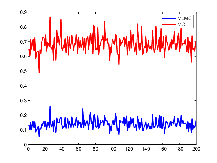
We actually repeat the whole procedure 200 times, and show on Figure 12 the 200 values of the relative errors that we found. We see that these errors are essentially the same for all the realizations. A gain in accuracy of the order of 5 is obtained when using the MLMC approach, for an equal cost:

{\mathbb{E}}(e_{MLMC})\approx 0.1411,\quad{\mathbb{E}}(e_{MC})\approx 0.6851.

The standard deviation of the MLMC error is also smaller:

{\rm std}_{MLMC}=0.0324,\quad{\rm std}_{MC}=0.0565.

Acknowledgments

A part of this work was done while YE was visiting ENPC and ITWM. YE is grateful for the support from ENPC and INRIA as well as Humboldt Foundation and ITWM. The research of CK was partially supported by the DFG Project IL 55/1-2. The work of FL is partially supported by ONR under Grant N00014-12-1-0383. FL warmly thanks the Fraunhofer Institute ITWM (where this work was initiated) and the Texas A & M University for their kind hospitalities.

Appendix A Appendix: weighted MLMC approach analysis

We estimate here the error associated to the weighted MLMC approach introduced in Section 4.2. To this aim, it is useful to introduce the function

\widetilde{u}=\sum_{l=1}^{L}\frac{\alpha_{l}}{M_{l}}\sum_{j=l}^{L}(M_{j}-M_{j+1})\left(u^{*}_{\eta_{j},H_{l}}-u^{*}_{\eta_{j},H_{l-1}}\right).

We indeed note that ${\mathbb{E}}\left(E^{L*}_{weighted}\right)={\mathbb{E}}(\widetilde{u})$ . The error between the computed quantity $E^{L*}_{weighted}$ and the exact quantity ${\mathbb{E}}(u^{*})$ is thus composed of a statistical error (the expectation of $E^{L*}_{weighted}$ is only approximately estimated) and of a systematic error, due to the fact that ${\mathbb{E}}\left(E^{L*}_{weighted}\right)={\mathbb{E}}(\widetilde{u})\neq{\mathbb{E}}(u^{*})$ . We successively estimate these two contributions.

Systematic error estimation

Following the same lines as in Section 3, we obtain that

\left\|\alpha_{1}u^{*}-\widetilde{u}\right\|\leq\sum_{l=1}^{L}{\cal E}_{l,l}\left[\alpha_{l}-\alpha_{l+1}\right]

where we have set $\alpha_{L+1}=0$ and $\displaystyle{\cal E}_{j,l}:=\left\|u^{*}-u^{*}_{\eta_{j},H_{l}}\right\|$ . Choosing now

\alpha_{l}=\sum_{j=l}^{L}\widetilde{\alpha}_{j}\frac{{\cal E}_{L,L}}{{\cal E}_{j,j}}

(22)

to equilibrate the terms in the above error bound, we get

\left\|\alpha_{1}u^{*}-\widetilde{u}\right\|\leq{\cal E}_{L,L}\sum_{l=1}^{L}\widetilde{\alpha}_{l}\quad\text{with}\quad\alpha_{1}=\sum_{j=1}^{L}\widetilde{\alpha}_{j}\frac{{\cal E}_{L,L}}{{\cal E}_{j,j}}.

As shown in Section 4.1, we have $\displaystyle{\cal E}_{j,l}\lesssim H_{l}+\left(\frac{\epsilon}{\eta_{j}}\right)^{\beta/2}+\frac{1}{\sqrt{m_{j}}}$ .

For the standard MC approach, the systematic error reads

\|u^{*}-u_{\widehat{\eta},\widehat{H}}\|\lesssim\widehat{H}+\widehat{\delta}.

To have the same systematic error, we choose the coarse grid size $\displaystyle\widehat{H}=\sum_{l=1}^{L}(\alpha_{l}-\alpha_{l+1})H_{l}$ and RVEs of size $\widehat{\eta}$ so that $\displaystyle\widehat{\delta}=\left(\frac{\epsilon}{\widehat{\eta}}\right)^{\beta/2}=\sum_{l=1}^{L}(\alpha_{l}-\alpha_{l+1})\delta_{l}$ .

Statistical error estimation

The statistical error of the weighted MLMC approximation satisfies

\left\|{\mathbb{E}}(\widetilde{u})-\sum_{l=1}^{L}\alpha_{l}E^{*}_{M_{l}}(u^{*}_{l}-u^{*}_{l-1})\right\|\lesssim\sum_{l=1}^{L}\frac{\alpha_{l}}{\sqrt{M_{l}}}(H_{l}+\delta_{l})+\frac{\alpha_{1}}{\sqrt{M_{1}}}.

To equate the error terms in the above sum, we choose

M_{l}=C\left(\frac{\alpha_{l}(H_{l}+\delta_{l})}{\gamma_{l}(\widehat{H}+\widehat{\delta})}\right)^{2}\ \text{for $l\geq 2$},\quad M_{1}=C\left(\frac{\alpha_{1}}{\gamma_{1}(\widehat{H}+\widehat{\delta})}\right)^{2},

(23)

for some constant $C$ and some parameters $\gamma_{l}$ . The statistical error then satisfies

\left\|{\mathbb{E}}\left(E^{L*}_{weighted}\right)-E^{L*}_{weighted}\right\|=O(\widehat{H}+\widehat{\delta}).

For the MC approach, we choose $\widehat{M}=C(\widehat{H}+\widehat{\delta})^{-2}$ independent realizations and thus get a statistical error of the same order.

Cost comparison

Now that we have chosen parameters such that the MC and the weighted MLMC approaches share the same accuracy, we are in position to compare their cost.

As above, the cost of solving the coarse scale problems is

W^{w-MLMC}_{\rm coarse}=\sum_{l=1}^{L}M_{l}H_{l}^{-2}\quad\text{and}\quad W^{MC}_{\rm coarse}=\widehat{M}\widehat{H}^{-2}.

The dominating part of the computational cost however lies in solving the local RVE problems. For the MC approach, we assume that we need to solve these problems at $\widehat{N}$ macroscopic points $x$ . We thus have

W^{MC}_{\rm RVE}=\widehat{M}\widehat{N}\left(\frac{\widehat{\eta}}{\epsilon}\right)^{2}=C\frac{\widehat{N}\widehat{\eta}^{2}}{\epsilon^{2}(\widehat{H}+\widehat{\delta})^{2}}.

For the weighted MLMC approach, we assume that, at each level $l$ , we solve local RVE problems at $N_{l}\leq H_{l}^{-2}$ macroscopic points (with $N_{1}<N_{2}<\cdots<N_{L}$ ). At each of these points, we only need to consider $M_{l}-M_{l+1}$ realizations. The computational work thus reads

W^{w-MLMC}_{\rm RVE}=\sum_{l=1}^{L}(M_{l}-M_{l+1})\left(\frac{\eta_{l}}{\epsilon}\right)^{2}N_{l}.

On Figure 13, we show the ratio of the works for solving the coarse problems and the RVE problems, as a function of the number of levels $L$ . The figure is made with the parameter $\beta=2$ (which corresponds to a Central Limit Theorem type convergence, see discussion below (10)). As on Figure 3, we consider two possible regimes for $\epsilon$ . We see that a significant gain is achieved even for moderate values of $L$ .

References

[1] A. Abdulle, A. Barth, and C. Schwab, Multilevel Monte Carlo methods for stochastic elliptic multiscale PDEs, preprint available at http://infoscience.epfl.ch/record/182185.
[2] A. Anantharaman, R. Costaouec, C. Le Bris, F. Legoll, and F. Thomines, Introduction to numerical stochastic homogenization and the related computational challenges: some recent developments. In W. Bao and Q. Du, editors, Multiscale modeling and analysis for materials simulation, Lecture Notes Series, Institute for Mathematical Sciences, National University of Singapore, vol. 22, pages 197–272, 2011.
[3] G. Bal. Homogenization in random media and effective medium theory for high frequency waves. Discrete and Continuous Dynamical Systems B, 8(2):473–492, 2007.
[4] A. Barth, C. Schwab, and N. Zollinger. Multi-level Monte Carlo finite element method for elliptic PDEs with stochastic coefficients. Numerische Mathematik, 119(1):123–161, 2011.
[5] P. Bastian, M. Blatt, A. Dedner, C. Engwer, R. Klöfkorn, R. Kornhuber, M. Ohlberger, and O. Sander. A generic grid interface for parallel and adaptive scientific computing. Part II: Implementation and tests in DUNE. Computing, 82(2–3):121–138, 2008.
[6] P. Bastian, M. Blatt, A. Dedner, C. Engwer, R. Klöfkorn, M. Ohlberger, and O. Sander. A generic grid interface for parallel and adaptive scientific computing. Part I: Abstract framework. Computing, 82(2–3):103–119, 2008.
[7] A. Bensoussan, J.-L. Lions, and G. Papanicolaou, Asymptotic analysis for periodic structures, Studies in Mathematics and its Applications, vol. 5. North-Holland Publishing Co., Amsterdam-New York, 1978.
[8] X. Blanc, R. Costaouec, C. Le Bris, and F. Legoll. Variance reduction in stochastic homogenization using antithetic variables. Markov Processes and Related Fields, 18(1):31–66, 2012 (preliminary version available at http://cermics.enpc.fr/ $\sim$ legoll/hdr/FL24.pdf).
[9] X. Blanc, R. Costaouec, C. Le Bris, and F. Legoll. Variance reduction in stochastic homogenization: the technique of antithetic variables. In B. Engquist, O. Runborg, and R. Tsai, editors, Numerical Analysis and Multiscale Computations, Lect. Notes Comput. Sci. Eng., Springer, vol. 82, pages 47–70, 2012.
[10] M. Blatt and P. Bastian. The iterative solver template library. In B. Kagstrüm, E. Elmroth, J. Dongarra, and J. Wasniewski, editors, Applied Parallel Computing. State of the Art in Scientific Computing, Lect. Notes Sci. Computing, Springer, vol. 4699, pages 666–675, 2007.
[11] A. Bourgeat and A. Piatnitski. Approximation of effective coefficients in stochastic homogenization. Annales de l’Institut Henri Poincaré (B) Probability and Statistics, 40(2):152–165, 2004.
[12] D.L. Brown, V.H. Hoang, and Y. Efendiev. An efficient hierarchical multiscale Finite Element method for Stokes equations in slowly varying media. SIAM MMS, to appear.
[13] R.E. Caflisch. Monte Carlo and Quasi-Monte Carlo methods. Acta Numerica, 7:1–49, 1998.
[14] J. Charrier, R. Scheichl and A.L. Teckentrup, Finite Element error analysis of elliptic PDEs with random coefficients and its application to Multilevel Monte Carlo methods, SIAM Journal on Numerical Analysis, in press.
[15] D. Cioranescu and P. Donato, An introduction to homogenization. Oxford Lecture Series in Mathematics and its Applications, vol. 17. The Clarendon Press, Oxford University Press, New York, 1999.
[16] K.A. Cliffe, M.B. Giles, R. Scheichl, and A.L. Teckentrup. Multilevel Monte Carlo methods and applications to elliptic PDEs with random coefficients. Computing and Visualization in Science, 14(1):3–15, 2011.
[17] R. Costaouec, C. Le Bris, and F. Legoll. Variance reduction in stochastic homogenization: Proof of concept, using antithetic variables. Bol. Soc. Esp. Mat. Apl., 50:9–27, 2010.
[18] A. Dedner, R. Klöfkorn, M. Nolte, and M. Ohlberger. A generic interface for parallel and adaptive scientific computing: Abstraction principles and the DUNE-FEM module. Computing, 90(3–4):165–196, 2010.
[19] Y. Efendiev. The Multiscale Finite Element Method (MsFEM) and its applications. PhD thesis, California Institute of Technology, 1999.
[20] M.B. Giles. Improved Multilevel Monte Carlo convergence using the Milstein scheme. In A. Keller, S. Heinrich, and H. Niederreiter, editors, Monte Carlo and Quasi-Monte Carlo Methods 2006, pages 343–358. Springer Berlin Heidelberg, 2008.
[21] M.B. Giles. Multilevel Monte Carlo path simulation. Operations Research, 56(3):607–617, 2008.
[22] A. Gloria and F. Otto. An optimal variance estimate in stochastic homogenization of discrete elliptic equations. Ann. of Probab., 39(3):779–856, 2010.
[23] S. Heinrich. Multilevel Monte Carlo methods. In S. Margenov, J. Wasniewski, and P. Yalamov, editors, Large Scale Scientific Computing, Lect. Notes in Computer Science, vol. 2179, pages 58–67, Springer, 2001.
[24] V.V. Jikov, S.M. Kozlov, and O.A. Oleinik. Homogenization of differential operators and integral functionals. Springer-Verlag, 1994.
[25] T. Kanit, S. Forest, I. Galliet, V. Mounoury, and D. Jeulin. Determination of the size of the representative volume element for random composites: statistical and numerical approach. International Journal of Solids and Structures, 40(13-14):3647–3679, 2003.
[26] G. Papanicolaou and S. Varadhan. Diffusion with random coefficients. Statistics and Probability: Essays in Honor of C.R. Rao, pages 547–552, North-Holland, Amsterdam, 1982.
[27] A.L. Teckentrup, R. Scheichl, M.B. Giles and E. Ullmann, Further analysis of Multilevel Monte Carlo methods for elliptic PDEs with random coefficients, arXiv preprint 1204.3476.
[28] V.V. Yurinskii. Averaging of symmetric diffusion in random medium. Sibirskii Mat. Zh., 27(4):167–180, 1986.

$\displaystyle\left\\|u^{*}_{H_{l}}-u_{l}\right\\|$	$\displaystyle\lesssim$	$\displaystyle\sqrt{{\mathbb{E}}\left[\left\|E_{m_{l}}(B_{l}^{})-{\mathbb{E}}\left(B^{}\right)\right\|^{2}\right]}$
	$\displaystyle\leq$	$\displaystyle\sqrt{{\mathbb{E}}\left[\left\|E_{m_{l}}(B_{l}^{})-{\mathbb{E}}(B^{}_{l})\right\|^{2}\right]}+\left\|{\mathbb{E}}(B^{}_{l})-{\mathbb{E}}\left(B^{}\right)\right\|$
	$\displaystyle\lesssim$	$\displaystyle\frac{1}{\sqrt{m_{l}}}\sqrt{{\mathbb{E}}\left[\left\|B_{l}^{}-{\mathbb{E}}(B^{}_{l})\right\|^{2}\right]}+\delta_{l}.$

	$\displaystyle E^{}_{M_{l}}(u^{}_{l}-u^{*}_{l-1})$	$\displaystyle:=$	$\displaystyle\frac{1}{M_{l}}\sum_{j=l}^{L}\left(\sum_{i=1}^{M_{j}-M_{j+1}}\left(u^{}_{\eta_{j},H_{l}}-u^{}_{\eta_{j},H_{l-1}}\right)(\omega_{i})\right)$
		$\displaystyle=$	$\displaystyle\frac{1}{M_{l}}\sum_{j=l}^{L}(M_{j}-M_{j+1})E_{M_{j}-M_{j+1}}(u^{}_{\eta_{j},H_{l}}-u^{}_{\eta_{j},H_{l-1}}),$