CORSIKA Implementation of Heavy Quark Production and Propagation in Extensive Air Showers
Abstract
Heavy quarks are commonly produced in current
accelerator experiments. Hence it is natural to think that they should be
likewise created in collisions with larger center of mass energies like
the ones involving ultra-high energy cosmic rays and atmospheric
nuclei. Despite this fact, a detailed treatment of heavy hadrons is missing in
Monte Carlo generators of Extensive Air Showers (EAS). It is a must to
improve the description of how heavy
flavours appear and evolve in atmospheric showers. With this goal in mind, we study two different models for heavy quark
production in proton-air collisions. We also analyze a dedicated treatment of heavy hadrons interactions
with atmospheric nuclei. This paper shows how those models have been
implemented as new options available in CORSIKA, one of the most used
EAS simulators. This new computational tool allows us to analyze the effects that the propagation of heavy
hadrons has in the EAS development.
Program summary
Title of program: corsika-6990-Heavy
Computer on which the program has been thoroughly tested: Intel-Pentium based Personal Computers
Operating system: Linux
Programming language used: FORTRAN77
Memory required to execute: 373 Mb
Other procedures used: NUCOGE [Linkai Ding, Evert Stenlund, Comput. Phys. Commu. 59 (1990) 313]
Nature of physical problem: Charmed and bottom hadron production and propagation inside Extensive Air Showers.
Solution method: Heavy quarks are produced according to two different production models. Propagation in the atmosphere
is handled using already present CORSIKA subroutines. New subroutines are written to simulate their interactions with
air nuclei.
Restrictions on the problem: Heavy quark production has only been implemented in the first interaction.
Running time and output file size: From 4.2 h and 120 Mb at eV
to 4.7 h and 170 Mb at eV, with thinning E(GeV).
1 Introduction
Charm and bottom quarks are copiously produced at accelerators ([1, 2, 3, 4]) and the physics involved in their production and hadronization processes is reasonably understood [5, 6]. If they are produced in the energy range probed at colliders, we expect them to be produced in the hadronic collisions taking place in Extensive Air Showers (EAS) too, since the most energetic cosmic rays reach energies of a few tens of EeV. At 0.01 EeV heavy hadrons reach their critical energies and their decay probabilities decrease rapidly. Decay lengths grow to considerable values: at 1017.5 eV they are of the order km for charmed and bottom hadrons. In addition, due to their larger masses, we expect heavy hadrons interactions with other hadrons to be more elastic on average, keeping a higher fraction of their energy after each interaction. Thus, above 0.1 EeV we expect the behavior of heavy hadrons to be very different from that at lower energies.
Heavy quarks can in principle be produced at any stage of the shower development, but it is only during the first interactions that they can be produced with a significant amount of energy (namely above their critical energies). Under those circumstances, they can penetrate deep into the atmosphere giving rise to additional contributions to the development of EAS.
Current Monte Carlo air shower simulators lack a full treatment of heavy hadrons. Charm production is not always addressed, and charmed particle propagation is to a large extent neglected. As for bottom particles, they are neither produced nor propagated and they are not included in the list of particles considered for simulation.
In this paper we address the question of how to implement the physics of heavy quarks inside the CORSIKA air shower simulator. In section 2 we summarize the production and propagation models we use for the explicit treatment of charmed and bottom hadrons in EAS. The structure of the simulation chain is discussed in section 3. In section 4 we analyze the effect of these modifications in the shower development. Details of the code implementation are presented in the appendices. Throughout this work we use the following programs and software packages:
- •
- •
the number of nucleons participating in hadron-air collisions is simulated using NUCOGE [11].
2 Physics of heavy hadron production and propagation
2.1 Production models
The production of heavy quarks at accelerator energies is explained by Quantum Chromodynamics. At cosmic rays collisions we are confronted with the problem of the energy scale, with collisions whose center of mass energies are of the order of 100 TeV. Accelerator data is several orders of magnitude below and therefore extrapolation over large ranges of energy is mandatory. However these extrapolations are prone to large uncertainties, as large as 40% [12]. To circumvent this difficulty, at the highest energies analysis based on effective theories are derived. The solution to this problem is not unique, and different regimes allow for different approaches, which in turn offer qualitatively correct results in certain limits. The Dual Parton Model [13], the Lund Fragmentation Model [14] or the Color Glass Condensate model [15] are some of the most well known effective theories. The latter is one of the most complete, supported by its analytic equivalence with the gluon-gluon fusion mechanism of the parton model [16].
However, not all features present in data are explained by this model. Leading particle asymmetries have been reported from different fixed target experiments. They show a strong correlation between the quantum numbers of the projectile and those of the final state hadron, whereas according to the QCD factorization theorem heavy quarks hadronize independently of the initial state [17]. For example, in () interactions with hadrons or nuclei, the () carries on average a larger fraction of energy than the () [18, 19]. Yet, the prediction stands that and quarks should be produced with identical energy distributions.
To explain this discrepancy theoretical models coincide in invoking a charm or bottom component inside the nucleon. The Meson-Cloud model [20], the Recombination Mechanism [21], or the Intrinsic Quark mechanism [19, 22, 23] are examples of these models, yet the nature and evolution of the heavy component differs between them. They produce similar results, but we will focus on the last model, which provides a simple mechanism for producing the flavor correlations present in data.
2.1.1 Color Glass Condensate
This is the first mechanism of heavy quark production we will briefly discuss and implement in CORSIKA (a more technical discussion of the model can be found in [24, 25]). In this model, a heavy flavor quark-antiquark pair is created through the fluctuation of the probing gluon. Charmed and bottom hadrons are formed from hadronization of those heavy quarks with sea quarks, in a mechanism called Uncorrelated Fragmentation. Any heavy hadron has the same probability of being formed from the heavy quarks produced. We assume that hadronization occurs without energy loss, and thus the differential production probability for charmed (bottom) hadrons is identical to that of charm (bottom) quarks. Those distributions can be seen in Fig. 1 (left), both scaled to the same integral.


2.1.2 Intrinsic Quark production
At leading order in QCD, heavy quarks are produced by the processes and (Fig. 1, right). When these heavy quarks arise from fluctuations of the initial state, its wave function can be represented as a superposition of Fock state fluctuations:
| (1) |
where is the hadron ground state, composed only by its valence quarks. When the projectile scatters in the target the coherence of the Fock components is broken and the fluctuations can hadronize, either with sea quarks or with spectator valence quarks. The latter mechanism is called Coalescence. For instance, the production of in p-N collisions comes from the fluctuations of the Fock state of the proton to . To obtain a in the same collision a fluctuation to would be required. Thus, since the probability of a five quarks state is larger than that of a 9 quarks state, production is favored over in proton reactions. The co-moving heavy and valence quarks have the same rapidity in these states but the larger mass of the heavy quarks implies they carry most of the projectile momentum. Heavy hadrons formed from these states can have a large longitudinal momentum and carry a large fraction of the primary energy [26], which is crucial for their propagation. The differential energy fraction distribution for some charmed and bottom hadrons can be seen in Fig. 2.


2.2 Physics of heavy hadron propagation
Charmed and bottom hadrons produced at accelerators are short-lived particles and decay before interacting. In accelerator experiments their presence is signalled through the detection of their final state products. To measure, for instance, -p interaction cross-sections, or the elasticity in B- interactions, one would need to be able to produce beams of these particles above their critical energies( eV). Acceleration to those energies is so far out of reach from a technological point of view. However, in collisions of cosmic rays with momenta in the range of the EeV it is possible to creat heavy hadrons with energies above their critical one. In this section we explain how we treat cross-sections, interactions lengths and elasticities in this ultra-high energy regime.
2.2.1 Interaction cross-sections and interaction lengths
Following the procedure explained in [29] we obtain the inelastic cross-sections for , D, and B in collisions with protons at rest, in an energy range going from eV to eV. To scale these cross-section to collisions with air nuclei we apply the following prescription used in CORSIKA11 1 The parameterization is inside the subroutine BOX2.. Let be the hadron-proton cross-section. Then, the hadron-air cross section is obtained as:
| (2) |
where
From these cross-sections we can obtain the associated mean interaction length as
| (3) |
In Fig. 3 we can see the resulting cross-sections (left) and interaction lengths (right) for heavy hadrons above eV. We use and cross-sections as representative of all charmed and bottom baryons, respectively. In the same way, D and B cross-sections are used for all charmed and bottom mesons. We adopt this criterion because, during their propagation, heavier baryons and mesons transform into these lighter states during the first steps of the shower development. For instance, () states rapidly decay into (), which continue propagating in the atmosphere.


2.2.2 Interaction model
The realistic implementation of heavy hadron propagation in EAS needs, apart from the values of cross-sections and interaction lengths, the elasticity distributions of their interactions. We use the models described in [29] for the propagation of charmed and bottom hadrons. We analyze the collisions of very energetic D (B) mesons and () baryons with protons at rest. Using PYTHIA, diffractive and partonic collisions of any q2 are considered to generate the corresponding elasticity distributions.
During their propagation in the atmosphere, heavy hadrons interact with air nuclei, and not with protons. PYTHIA deals with hadron-nucleon collisions based on the Lund string model, but so far there is no agreement on how hadron-nucleus collisions should be treated within this model. We will use the method described in [30], which is the approach SIBYLL takes.
After a hadron-nucleon collision we find a leading hadron, carrying the largest fraction of the primary energy, and a series of secondary particles, sharing the rest of the energy. In a simplistic setting we could picture a hadron-nucleus interaction as a series of independent hadron-nucleon collisions with every nucleon composing the nucleus. As a result, the number of low energy secondaries produced would rise, increasing with each consecutive collision. Even though this is the behavior we would expect, the underlying assumptions are not correct. First, the time scales of the projectile traversing the nucleus and that of the recombination of partons inside the proton are fairly different, the former being much shorter. Thus, there is no time for the proton to recombine and suffer a second hadron-nucleon collision before it exits the nucleus. In addition, when a hadron collides with an air nucleus, not every nucleon within will participate in the interaction.
To compute the number of nucleons participating in the interaction, NA, we use the FORTRAN routine NUCOGE, where the probability of an inelastic hadron-nucleon hit is determined by the choice of the hadron-nucleon overlap function. A detailed explanation of how the program works can be found in [11]. The next step is deciding the nature of the hadron-nucleus interaction, either diffractive or partonic. The probability of a diffractive interaction, pdiff, is different for each projectile. In the case of charmed hadrons it is 0.30 for and 0.32 for D. Turning to bottom hadrons, the values are 0.26 for and 0.29 for B. Let ND be the number of nucleons interacting diffractively. We will consider that the interaction is diffractive if, and only if, the NA nucleons interact diffractively (NNA). If NNA, we consider that the collision is non-diffractive with NNND participating nucleons. To treat the inelastic interaction of a heavy hadron, with energy , with an air nucleus we use the following prescription:
- •
First, from the NW participating nucleons, all but one are split in quark-diquark pairs, i.e we have N pairs and one unbroken nucleon.
- •
Then, N quark-antiquark pairs are generated in the projectile, with total energy .
- •
The partonic interaction occurs between the projectile, with energy , and the nucleon in the target that remains unaltered.
- •
The quark-antiquark pairs are matched with the quark-diquark pairs and hadronize.
Both the partonic interaction and the hadronization are performed by PYTHIA. As a final state, we find the particles resulting from the hard interaction plus all the particles coming from the hadronization of the N pairs formed.
The main effect of the transition from hadron-nucleon to hadron-nucleus collisions is increasing the multiplicity of produced particles, and decreasing their elasticity. In Fig. 4 we show the effect of the transition from hadron-proton (dashed line) to hadron-air (solid line) collisions in case a is used as the probing projectile. All distributions are scaled to the same integral. In Fig. 4(a) and Fig. 4(b) we observe that the multiplicity of pions and kaons is larger in collisions with air. At the same time (Fig. 4(c) and Fig. 4(d)) the energy transferred to the pion component barely rises and thus the average elasticity per secondary particle is smaller (by a factor 1.5): a larger number of particles is sharing roughly the same amount of energy.
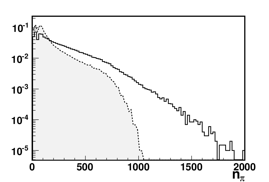


Interacting with air nuclei rather than with protons also affects the leading hadron. In Fig. 5 we can see the elasticity distributions of the leading charmed and bottom hadrons after collisions with protons compared to those where the collisions take place off air nuclei (solid lines).
| p | 0.62 | 0.65 | 0.72 | 0.75 |
| Air | 0.56 | 0.59 | 0.68 | 0.72 |


All distributions are scaled to the same integral. Regarding the comparison between charmed and bottom hadrons collisions, we find that the latter are, on average, more elastic than the former. That is because the heavy quark composing the hadron behaves as a spectator most of the time, losing a small amount of its energy in the interaction. In addition, the fraction of the heavy hadron energy carried by the heavy quark is proportional to the heavy quarks mass.
Collisions with air nuclei are also more inelastic than collisions with protons. In hadron-nucleus collisions there might be more than one nucleon involved. Interacting with more nucleons increases the number of soft secondaries, and decreases the energy fraction carried away by the leading particle. The mean elasticity values for collisions with protons and air can be found in Table 1.
3 Simulation chain and code implementation
In this section we describe the different steps involved in the Monte Carlo simulation of heavy hadrons in EAS and reference the subroutines modified or newly written. The reader can find a summary of the modifications made to the CORSIKA source code in Appendix C. As we mentioned in section 1, Monte Carlo simulators do not handle charmed hadrons production or, if they do, they are not propagated. In the case of bottom hadrons, they are not even included in the list of particles recognized by the programs. Our goal is to implement these particles, such that they are eligible candidates for production and propagation.
The simulation chain consists of several steps. Initially, we simulate the primary particle first interaction, choosing whether charmed hadrons, bottom hadrons or none of them are produced in the collision. The propagation of heavy hadrons across the atmosphere takes place along with the rest of the shower, but according to the interaction model described in section 2.2.2. The decay of both charmed and bottom hadrons is performed by PYTHIA.
3.1 First interaction
Heavy quarks can be produced in any of the collisions taking place along the shower development, provided the interaction is energetic enough. However we restrict our interest only to heavy hadrons produced in the first interaction of the primary particle with an atmospheric nucleus. Charmed and bottom hadrons produced in subsequent interactions are much less energetic and therefore their influence in the longitudinal development of the shower will be small. And, even though they could be produced deeper in the atmosphere, it is the energy, and not the production depth, that rules the propagation. To check this, we simulate and mesons with a uniform distribution in logE/eV. The production depth corresponds to the depth of the proton first interaction, distributed as
| (4) |
In Fig. 6 (left) we plot the mean number of interactions suffered by the and in the atmosphere before decaying as a function of the initial meson energy, for different ranges of production depths. In Fig. 6 (right) we can find the mean number of interactions suffered by the , as a function of X0, for different primary energy ranges. The number of interactions suffered before decay increases rapidly as the meson initial energy grows, almost independently of . Whereas for fixed energies, the number of interactions is roughly constant with growing production depth.


The subroutine COLLIDE produces the charmed or bottom hadrons right after the primary proton first interaction. As we mentioned in section 2.1.1 heavy hadrons in the Color Glass Condensate model are formed via fragmentation. Thus, all heavy hadrons are formed with equal probability. In the case of Intrinsic Quark production, the proton develops a fluctuation to a 5- or 7-particle state before the collision with an air nucleus. We will not consider higher fluctuations. During the collision, each of the heavy quarks composing the fluctuation will independently hadronize, either by coalescence or fragmentation, with probability 50%. However, the allowed final states will not always be independent: when hadronization occurs by fragmentation any hadron can be formed; upon hadronization by coalescence, the accessible states are limited by the quark content of the fluctuation. For instance, if the proton develops a fluctuation, no bottom hadrons containing a quark can be formed by coalescence. Thus, the distributions of the primary energy fraction that goes into different hadrons will be different (see for example Fig. 2).
3.2 Propagation
After their production, the heavy hadrons generated at the first interaction have to be propagated. This is the process largely neglected in air shower simulators. As CORSIKA has been modified to recognize particles with bottom quarks, both charmed and bottom hadrons can be propagated using the standard machinery built in CORSIKA. During their propagation, these particles will interact with nuclei in the atmosphere or will decay in flight. Whether any of these happens depends on the values of the interaction and decay lengths. The mean interaction length in units of depth is given by Eq. 3. The interaction lengths for charmed and bottom hadrons are plotted in Fig. 3 (right). The mean decay length, i.e the mean distance a particle traverses before it decays, in units of distance is given by:
| (5) |
where is the particle mean life-time and its mass. In CORSIKA, the actual values for the interaction and decay lengths are sampled from the following exponential distributions:
| (6) | |||||
| (7) |
If , where is the decay length expressed in depth units, the particle travels a distance and decays. Else, the particle travels before interacting with an atmospheric nucleus. Energy losses during the particle time-of-flight are treated by CORSIKA standard routines.
3.3 Interaction
As heavy hadrons cross the atmosphere, they will collide with atmospheric nuclei. We treat the collisions according to the model described in section 2. The new subroutine HEPARIN links with the PYTHIA routines that treat the interaction of heavy hadrons with air nuclei, instead of calling the high-energy hadronic model chosen during compilation. It calculates the number of interacting atmospheric nucleons using the function NNY and assigns whether the interaction is diffractive or partonic. After each collision numerous particles are generated, and usually the particle containing the heavy quark carries away the largest energy fraction. All the collision products are injected back to the CORSIKA stack using PYTSTO and tracked as any other particle that contributes to the shower development.
3.4 Decay
During their propagation in the atmosphere the heavy hadrons will lose energy due to bremsstrahlung and ionization, but specially because of their collisions with nuclei. The decrease in energy modifies the values of both the interaction and decay lengths, rising the former and reducing the latter, and thus increasing the decay probability. At the same time, the particle approaches ground and the atmosphere grows thicker, reducing the distance between interactions. The interplay of these effects will determine where the decay occurs.
The decay of both charmed and bottom particles is performed within CORSIKA. BTTMDC, a new subroutine, is called to treat the decay of bottom hadrons. It is analogous to the already existing CHRMDC CORSIKA routine.
4 Effects on shower propagation
We have used the modified CORSIKA package described in previous sections to generate large statistical samples of showers where charm or bottom quarks are produced in the first interaction. For each heavy quark, we have generated a library that contains more than one hundred thousand events. Our goal is to understand how the presence of a heavy hadron could affect fundamental parameters of the cascade development like the shape of its longitudinal profile, the number of particles reaching ground, the position and amplitude of the shower maximum, etc. Heavy hadrons propagating with an energy above their critical one will fly over long paths. After several elastic interactions, we expect them to deposit their remaining energy deep in the atmosphere and some might even reach ground. In the case the heavy hadron carries a significant fraction of the energy of the primary particle that created the shower, one naturally expects that both the size and the shape of the cascade will be altered. The larger the energy of the heavy component, the more accentuated these effects will be.
Let us analyze the case where the energy deposition in the shower is shifted to larger depths. The position and the amplitude of the shower maximum will be affected. The number of particles at maximum will decrease, while at the same time the number of particles that reach ground will increase. In Fig. 7 (left) we plot the ratio of the number of particles at shower maximum with respect to the number of particles at ground. This ratio is plotted as a function of the energy fraction carried away by the heavy hadrons produced in the first interaction. As this fraction grows, the ratio decreases, which means that a component of the shower is being displaced to larger depths. The bands show the deviation. For comparison, we superimpose (solid symbol) the average value deviation for proton showers where heavy quark production has been turned off.


For similar reasons shower profiles with a leading heavy hadron must be wider on average, with larger RMS. This effect must increase with rising fractions of the energy carried away by the heavy hadrons. As shown in Fig. 7 (right) our hypothesis is confirmed by simulations. The mean RMS of the showers increases with the energy fraction transferred to the heavy quark. For reference, we plot the expected RMS value along with its deviation for proton showers where no heavy quark production is allowed.
To illustrate further how the energy of the leading heavy hadron influences the development of the shower, we plot in Fig. 8 and Fig. 8 the mean eV shower profiles for proton showers with charm production and bottom production, respectively. We compared them to those of proton showers with no heavy quark production. We divide the simulated events in two samples: one in which the heavy component carries less than 50% of the proton energy and its complementary set. In the case of charm production, the average profile is only slightly different of that of proton showers. However, in the case of bottom production, both samples are different when compared to protons: they show a smaller number of particles at maximum and on average they are deeper. We can see the differences more clearly if we inspect individual profiles. In Fig. 9 we show the fluctuations in the shower profile due to the propagation of bottom hadrons. When the heavy component carries less than 50% of the proton energy the effect is small, the shower profiles (Fig. 9(b)) resembling those of proton showers with no heavy quark production (Fig. 9(a)). For energy fractions above 50% the effect is clearly noticeable (Fig. 9(c)). In Fig. 9(d) we highlight some showers from Fig. 9(c) whose profiles are specially anomalous. These showers show a slower development resulting either on a plateau or on a broader maximum.
We can also consider extreme cases where the heavy hadron reaches ground. This happens when numerous but very elastic interactions take place, or if the hadron interacts only a few times with long distances traveled between interactions. For EAS at =60o the atmosphere has a slant depth of approximately 1760 g cm-2. In Fig. 8 we plot the probability of decaying above 1700 g cm-2 (equivalent to reaching ground) as a function of the production energy for different bottom hadrons (charmed hadrons have negligible probabilities of reaching ground, below 0.5% at all energies, and are not included in the plot). In those cases we have a standard longitudinal profiles whose measured energy is smaller than that of the primary particle, the rest of the energy being carried away by the heavy hadron and not deposited in the atmosphere.


The discussion of whether the detection of heavy quarks in EAS is feasible lies certainly beyond the scope of the present study. But we hope that some of the features discussed in this section can be used in present or future cosmic ray observatories to reveal that heavy hadrons are produced in the atmosphere following the collisions of ultra-high energy cosmic rays.
5 Conclusions and prospects
We discussed the modifications performed in CORSIKA to create and propagate heavy hadrons. We have written specific subroutines to simulate their production during the first stage of an air shower development, and to treat their collisions with air nuclei. These subroutines can be activated and deactivated through a set of keywords in the CORSIKA control datacard. Our modifications have been incorporated into the last official release of the CORSIKA package (version 7.3500) [31].
The collisions of heavy hadrons with air turn out to be very elastic, with elasticity mean values above 50% in all cases. If heavy hadrons are produced with enough energy and they retain a high fraction of their initial energy after a collision, they will interact again rather than decaying. If a series of elastic interactions occur, the propagation of the heavy hadrons will likely have observable effects on the shower development.
Acknowledgments
We thank M. Masip and J.I. Illana for the theoretical input and discussions. We also thank D. Heck for his comments and reviews on the code modifications. The assistance of G. Rubio and M.D. Serrano with shower simulations is warmly acknowledged. This work has been partially supported by MICINN of Spain (FPA2009-07187) and by Junta de Andalucía (FQM 330).
Appendix Appendix A Particles considered and particle codes
The bottom quark is not considered in CORSIKA because none of the hadronic interaction models it implements produces bottom hadrons. If we want CORSIKA to propagate bottom hadrons, we first have to include them as eligible particles. The last particle included is , with code 173. We use the empty codes starting from 176 to include the new bottom hadrons. Bottom mesons and their antiparticles are identified by codes from 176 to 183. , , and baryons and their antiparticles have codes from 184 to 197. Only ground states of the particles have been introduced. Details on the particle codes, masses and lifetimes, obtained from the Particle Data Book [32], are shown in Table 2.
Appendix Appendix B Input file
CORSIKA reads a series of keywords to select the parameters of the simulations. These keywords have to be provided by the user as an input file. What follows is an example of a simple input file: in addition to the standard keywords, we have underlined those keywords needed to use the subroutines that control the physics of heavy hadron production and propagation:
- •
COLLDR determines the type of the heavy quarks produced during the first interaction (first argument), and the production mechanism (second argument). The first argument accepts the values 1 for charm production, 2 for bottom production or 0 in case the first interaction is simulated by the chosen hadronic interaction model (be it SIBYLL, QGSJET, …). The second one takes the values 1 for production via the Color Glass Condensate model, or 3, for production using the Intrinsic Quark model.
- •
SIGMAQ takes four arguments, the cross-sections (in mb) for interaction with protons of charmed mesons, charmed baryons, bottom mesons and bottom mesons, respectively. If the values are equal to 0 the parameterization shown in figure 3 is used.
- •
PROPAQ toggles the propagation of heavy hadrons with the new subroutines. If equal to 0, the propagation of heavy hadrons is performed by the high energy interaction model. If equal to 1, the propagation is dealt with using HEPARIN.
Appendix Appendix C Source code modifications
New functions have been written to perform specific parts of the simulation and some others have been modified inside
the source code to allow the propagation of the new particles. We list the files that have been modified,
those new files added, and overview the changes made to the code.
The directory corsika-6990/src/ contains the main source files needed to run CORSIKA. Inside the file corsika.F we have made several modifications to already present subroutines:
- •
DATAC reads the CORSIKA input file. This subroutine has been modified to accept the new keywords described in Appendix B.
- •
the subroutine NUCINT selects the type of interaction process according to the particle energy. Now it includes a call to the new subroutine COLLIDE, to simulate the first interaction with production of heavy hadrons. The selection of interaction or decay routines for different particles types is extended to treat bottom hadrons. Both charmed and bottom hadrons interactions are treated in the new subroutine HEPARIN.
- •
PAMAF initializes the masses in GeV, the electric charge in electron charge units and the mean life-times in s of the particles defined in CORSIKA. We modify it to hold the bottom hadrons defined in Appendix A as well.
- •
BOX2 determines the point of interaction or decay for any particle. It now uses the interaction cross-sections of charmed particles with air shown in Fig. 3 to calculate their interaction lengths and whether they decay or interact. It has been extended to treat bottom hadrons as well.
- •
PYTSTO transports the particles resulting from PYTHIA to the CORSIKA stack. It is modified to accept bottom hadrons too.
We have also added new subroutines:
- •
HEPARIN links with the PYTHIA routines that treat the interaction of heavy hadrons with air nuclei, instead of calling the high-energy model chosen during compilation.
- •
NNY samples the number of interacting nucleons in the collisions of heavy hadrons with air nuclei. The sampled distributions are obtained using a modified version of NUCOGE [11].
- •
BTTMDC is called to perform the decay of bottom hadrons.
Some of these modifications need the definition of new variables. These have been included in the header file
corsika.h.
The file qgsjet01c.f simulates the physics of the model QGSJET01c. We have modified it to suppress the production of heavy quarks
during the first interaction. Thus, only COLLIDE (see below) produces them at that step of the shower.
The directory corsika-6990/pythia contains all the PYTHIA routines called during the simulation of the shower. The source files of some of the new subroutines are here:
- •
the subroutine COLLIDE, in the file collider.f, produces the charmed or bottom hadrons at the first proton interaction. We assume that the first interaction can be described as the superposition of the shower generated by the heavy hadrons ( and ) and the shower started by a proton of energy . We use a proton as a primary and, once the depth of the first interaction () has been computed, we generate the pair and at depth , sampling the fractions of the proton energy carried away () from the corresponding distributions. The energy of the proton is scaled to and the proton shower starts at . The particles are transferred to the CORSIKA stack using the subroutine PYTSTO. The rest of the shower development follows the usual procedure. The type of particle produced (charm or bottom) and the production model (Color Glass Condensate or Intrinsic Quark) are chosen setting new keywords in the datacard (see Appendix B).
- •
the subroutines CHABADIF, CHABAPAR, CHAMEDIF, CHAMEPAR, BOBADIF, BOBAPAR, BOMEDIF and BOMEPAR (defined in the files with the same names and extension .f) are called from HEPARIN to treat the diffractive and partonic interactions of heavy hadrons. The interactions are simulated according to the model described in section 2.
The processes included in the subroutines above need the modification of two PYTHIA source files, pypdfu.f and pyspli.f.
| Particle | Particle | Particle | Particle | Particle | Particle | Particle | Particle |
|---|---|---|---|---|---|---|---|
| code | name | mass | life-time | code | name | mass | life-time |
| [GeV] | [s] | [GeV] | [s] | ||||
| 176 | 5.27958 | 1.519 | 187 | 5.788 | 1.49 | ||
| 177 | 5.27925 | 1.641 | 188 | 5.7911 | 1.56 | ||
| 178 | 5.27925 | 1.641 | 189 | 6.071 | 1.1 | ||
| 179 | 5.27958 | 1.519 | 190 | 5.6194 | 1.425 | ||
| 180 | 5.36677 | 1.497 | 191 | 5.8155 | 1.3 | ||
| 181 | 5.36677 | 1.497 | 192 | 5.8113 | 1.68 | ||
| 182 | 6.277 | 0.453 | 193 | 5.788 | 1.49 | ||
| 183 | 6.277 | 0.453 | 194 | 5.7911 | 1.56 | ||
| 184 | 5.6194 | 1.425 | 195 | 6.071 | 1.1 | ||
| 185 | 5.8155 | 1.3 | 196 | 5.8155 | 0 * | ||
| 186 | 5.8113 | 6.8 | 197 | 5.8155 | 0 * |
References
- [1] D. Prindle. Heavy Flavor and Jets at RHIC. Nuclear Physics A, 862-863(0):71–77, 2011.
- [2] Yu. Guz. Studies of open charm and charmonium production at LHCb. Nuclear Physics B - Proceedings Supplements, 207-208(0):355–358, 2010.
- [3] J. Schieck. Heavy flavour measurements in ATLAS and CMS. arXiv:1205.4153 [hep-ex].
- [4] E. Prencipe. Heavy Spectroscopy at BaBar. Nuclear Physics B - Proceedings Supplements, 181-182(0):333–337, 2008.
- [5] J. Beringer et al. 2012 Review of Particle Physics. Phys. Rev. D, 86(010001), 2012.
- [6] C. Lourenço and H.K. Wöhri. Heavy-flavour hadro-production from fixed-target to collider energies. Physics Reports, 433(3):127–180, 2006.
- [7] D. Heck. Report FZK 6019. http://www-ik.fzk.de/physics-description/corsika-phys.html, 1998.
- [8] N.N. Kalmykov, S.S. Ostapchenko, and A.I. Pavlov. Quark-gluon-string model and EAS simulation problems at ultra-high energies. Nuclear Physics B - Proceedings Supplements, 52(3):17–28, 1997.
- [9] A. Fassò, A. Ferrari, S. Roesler, P.R. Sala, F. Ballarini, A. Ottolenghi, G. Battistoni, F. Cerutti, E. Gadioli, M.V. Garzelli, A. Empl, and J. Ranft. The physics models of FLUKA: status and recent development. Computing in High Energy and Nuclear Physics (CHEP03), La Jolla, Ca, USA, 2003.
- [10] A. Fassò, A. Ferrari, J. Ranft, and P.R. Sala. Report CERN-2005-10 (2005).
- [11] L. Ding, E. Stenlund. A Monte Carlo program for nuclear collision geometry. Computer Physics Communications, (59):313–318, 1990.
- [12] M. Cacciari, S. Frixione, M. L. Mangano, P. Nason, and G. Ridolfi. QCD analysis of first b cross section data at 1.96 TeV. Journal of High Energy Physics, 2004(07):033, 2004.
- [13] A. Capella, U. Sukhatme, C.-I. Tan, and J. Tran Thanh Van. Dual parton model. Physics Reports, 236(4–5):225–329, 1994.
- [14] B. Andersson, G. Gustafson, G. Ingelman and T. Sjöstrand. Parton fragmentation and string dynamics. Physics Reports, 97(2-3):31–145, 1983.
- [15] V. P. Gonçalves and M. V. T. Machado. Parton Saturation approach in heavy quark production at high energies. Modern Physics Letters A (MPLA), 19(34):2525–2539, 2004.
- [16] J. Raufeisen and J.-C. Peng. Relating the parton model and color dipole formulation of heavy quark hadroproduction. Phys. Rev. D, 67:054008, 2003.
- [17] J. Qiu and G. Sterman. Power corrections in hadronic scattering (II). Factorization. Nuclear Physics B, 353(1):137–164, 1991.
- [18] E. Norrbin and R. Vogt. Bottom Production Asymmetries at the LHC. Report number: LU TP 00-10, LBNL-45275.
- [19] R. Vogt and T. Gutierrez. Leading charm in hadron-nucleus interactions in the intrinsic charm model. Nucl. Phys. B, 539:189–214, 1999.
- [20] F. S. Navarra, M. Nielsen, C. A. A. Nunes, and M. Teixeira. Intrinsic charm component of the nucleon. Phys. Rev. D, 54:842–846, Jul 1996.
- [21] J.C. Anjos, J. Magnin, G. Herrera. On the intrinsic charm and the recombination mechanism in charm hadron production. Physics Letters B, (523):29–34, 2001.
- [22] R. Vogt and S.J. Brodsky. QCD and intrinsic heavy quark predictions for leading charm and beauty hadroproduction. Nuclear Physics B, 438(1–2):261–277, 1995.
- [23] E. Norrbin and R. Vogt. Bottom Production Asymmetries at the LHC. arXiv:hep-ph/0003056 [hep-ph], 2000.
- [24] V. P. Gonçalves and M. V.T. Machado. Saturation physics in ultra high energy cosmic rays: heavy quark production. Journal of High Energy Physics, 2007(04):028, 2007.
- [25] E.R. Cazaroto, V.P. Gonçalves, and F.S. Navarra. Heavy quark production at LHC in the color dipole formalism. Nuclear Physics A, 872(1):196–209, 2011.
- [26] N. Sakai, P. Hoyer, C. Peterson and S.J. Brodsky. The intrinsic charm of the proton. Phys. Lett. B, 93:451–455, 1980.
- [27] R. Vogt. Charm Production in Hadronic Collisions. Nuclear Physics A, 553:791–798, 1993.
- [28] R. Vogt, S.J. Brodsky. Charmed hadron asymmetries in the intrinsic charm coalescence model. Nuclear Physics B, 478:311–332, 1996.
- [29] A. Bueno, A. Gascón, J.I. Illana and M. Masip. Propagation of B mesons in the atmosphere. Journal of Cosmology and Astroparticle Physics, 2012(02):028, 2012.
- [30] R. S. Fletcher, T.K. Gaisser, P. Lipari, T. Stanev. SIBYLL:An event generator for simulation of high energy cosmic ray cascades. Physical Review D, 50(9):5710–5726, 1994.
- [31] http://www ik.fzk.de/corsika/usersguide/corsika_tech.html. .
- [32] K. Nakamura et al. (Particle Data Group). Review of Particle Physics. Journal of Physics G: Nuclear and Particle Physics, 37(7A):075021, 2010.