What’s Up in the Milky Way? The Orientation of the Disc Relative to the Triaxial Halo
Abstract
Models of the Sagittarius Stream have consistently found that the Milky Way disc is oriented such that its short axis is along the intermediate axis of the triaxial dark matter halo. We attempt to build models of disc galaxies in such an ‘intermediate-axis orientation’. We do this with three models. In the first two cases we simply rigidly grow a disc in a triaxial halo such that the disc ends up perpendicular to the global intermediate axis. We also attempt to coax a disc to form in an intermediate-axis orientation by producing a gas+dark matter triaxial system with gas angular momentum about the intermediate axis. In all cases we fail to produce systems which remain with stellar angular momentum aligned with the halo’s intermediate axis, even when the disc’s potential flattens the inner halo such that the disc is everywhere perpendicular to the halo’s local minor axis. For one of these unstable simulations we show that the potential is even rounder than the models of the Milky Way potential in the region probed by the Sagittarius Stream. We conclude that the Milky Way’s disc is very unlikely to be in an intermediate axis orientation. However we find that a disc can persist off one of the principal planes of the potential. We propose that the disc of the Milky Way must be tilted relative to the principal axes of the dark matter halo. Direct confirmation of this prediction would constitute a critical test of Modified Newtonian Dynamics.
Keywords:
Galaxy: evolution – Galaxy: formation – Galaxy: halo – Galaxy: kinematics and dynamics – Galaxy: structure – galaxies: haloes1 Introduction
Dark matter haloes in purely collisionless simulations are generally triaxial (Bardeen et al., 1986; Barnes & Efstathiou, 1987; Frenk et al., 1988; Dubinski & Carlberg, 1991; Jing & Suto, 2002; Bailin & Steinmetz, 2005; Allgood et al., 2006) with typical axial ratios and (where are the short, intermediate and long axes, respectively). Observations instead find rounder haloes (Schweizer et al., 1983; Sackett & Sparke, 1990; Franx & de Zeeuw, 1992; Huizinga & van Albada, 1992; Buote & Canizares, 1994; Kuijken & Tremaine, 1994; Franx et al., 1994; Olling, 1995; Kochanek, 1995; Bartelmann et al., 1995; Olling, 1996; Schoenmakers et al., 1997; Koopmans et al., 1998; Olling & Merrifield, 2000; Andersen et al., 2001; Buote et al., 2002; Oguri et al., 2003; Iodice et al., 2003; Debattista, 2003; Barnes & Sellwood, 2003; Diehl & Statler, 2007; Spekkens & Sellwood, 2007; Banerjee & Jog, 2008). This discrepancy is most likely accounted for by the fact that haloes become rounder when baryons condense within them (Dubinski, 1994; Kazantzidis et al., 2004; Debattista et al., 2008; Zemp et al., 2012; Bryan et al., 2013). This is mainly due to a change in both the type and shape of orbits (Valluri et al., 2010). Nonetheless models predict that haloes remain triaxial beyond kpc, which, however, is a region that is poorly constrained by observations.
The Sagittarius dwarf tidal stream, which extends to from the Galactic Centre, has been used to constrain the shape of the Milky Way’s halo with varying results. Noting that the tidal debris is distributed on a great circle, Ibata et al. (2001) concluded that the halo is nearly spherical. Likewise Fellhauer et al. (2006) argued that the position of the bifurcation in the tidal stream, which they interpreted as two wraps of the stream, can be explained if the halo is close to spherical. Martínez-Delgado et al. (2004) and Johnston et al. (2005) instead found a mildly oblate halo () flattened in the same sense as the disc. Helmi (2004a) meanwhile argued that the trailing part of the Sagittarius Stream is too dynamically young to provide a stringent constraint. Using instead the leading stream, Helmi (2004b) found evidence for a prolate halo with and with its long axis perpendicular to the disc. Law et al. (2009) were the first to demonstrate that simultaneously fitting the density and kinematics of the Sagittarius Stream requires a triaxial (rather than oblate/prolate) potential. A surprising property of this potential is that its intermediate axis is aligned with the short axis of the disc (a relative orientation we will refer to as the ‘intermediate-axis orientation’). Law & Majewski (2010, hereafter LM10) presented a suite of -body simulations of the tidal disruption of the Sagittarius dwarf in a fixed potential. The simulations were compared with a large number of constraints including (i) the position and velocity of the Sagittarius dwarf with its velocity vector in the orbital plane of the young trailing tail, (ii) the radial velocity and velocity dispersion in the trailing tidal tail and (iii) the angular location, width and radial velocities of the leading tail. The best-fitting model is in the intermediate-axis orientation with and between 20 and 60 kpc, and with the major and minor axes in the plane of the disc. An analysis by Deg & Widrow (2013) that varies also the parameters of the bulgedisc of the Milky Way still finds a disc in the intermediate-axis orientation. Recent extended mapping of the Sagittarius Stream in the Southern Galactic hemisphere finds a stream consistent with the LM10 model (Slater et al., 2013).
Triaxial potentials are populated by box orbits (which get arbitrarily close to the centre of the potential) and tube orbits (which have a fixed sense of rotation relative to one of the principal axes). The stability of tube orbits about each of the principal axes of a triaxial potential has been studied extensively: tube orbits are stable around the short and long axes, but not around the intermediate axis (Heiligman & Schwarzschild, 1979; Goodman & Schwarzschild, 1981; Wilkinson & James, 1982), even when planar (Adams et al., 2007; Carpintero & Muzzio, 2012). Figure rotation gives rise to warped planes of stable loop orbits capable of supporting discs (Binney, 1978; Heisler et al., 1982; Magnenat, 1982; Lake & Norman, 1983; Durisen et al., 1983; Steiman-Cameron & Durisen, 1984; Martinet & de Zeeuw, 1988; Habe & Ikeuchi, 1985; Habe & Ikeuchi, 1988), but the level of figure rotation of dark matter haloes is found to be on average in cosmological dark-matter-only simulations (Bailin & Steinmetz, 2004). In semi-cosmological models, Aumer & White (2013) showed that discs are most stable when the angular momentum is aligned with the minor axis of the halo. The model of LM10 therefore challenges the view that the instability of intermediate-axis tube (IAT) orbits prohibits discs from forming in this orientation. One way in which this discrepancy might be resolved is if in the vicinity of the disc it dominates the net potential, which becomes flattened like the disc. Then the near-circular orbits in the disc are orbiting around the local short axis of the potential, and therefore in a stable configuration (Johnston, private communication).
In this paper we show that discs are unable to persist in an intermediate-axis orientation. We use both simulations in which discs are grown inside isolated triaxial haloes as well as a simulation of a galaxy forming out of gas with angular momentum about the intermediate axis of a triaxial halo. In Section 2 we discuss the methods used in this paper, including the initial conditions of the stars, dark matter and gas. Section 3 presents the evolution of the models. We draw our conclusions in Section 4. Appendix A presents our interpretation for why the intermediate-axis orientation is unstable based on an orbital study.
2 Numerical Methods
2.1 Constructing collisionless initial conditions
As in Debattista et al. (2008), we formed triaxial haloes via the merger of three or more spherical haloes (Moore et al., 2004). The mergers, and all subsequent collisionless simulations, were evolved with pkdgrav (Stadel, 2001), an efficient, multi-stepping, parallel treecode. The spherical haloes were generated from a distribution function using the method of Kazantzidis et al. (2004) with each halo composed of two mass species arranged on shells. The outer shell has more massive particles than the inner one, increasing the effective resolution in the centre. As shown in Debattista et al. (2008), a large part of the particle mass segregation persists after the mergers and the inner region remains dominated by the lower mass particles.
We produced two dark-matter-only triaxial haloes, which we refer to as A and C; halo A was presented already in Debattista et al. (2008). These haloes were constructed from two consecutive mergers. In both cases the first merger placed two identical spherical concentration haloes 800 kpc apart approaching each other at 50 , producing a prolate merged halo. Halo A was generated by the head-on merger of two copies of this remnant halo starting at rest 400 kpc apart. For halo C, after the first merger, a third spherical halo, with , was merged from 100 kpc along the first remnant’s minor axis. This halo itself had two mass species different from those of the halo. The top two panels of Fig. 1 plot the shape and triaxiality of these two haloes, measured as described in Debattista et al. (2008) (Zemp et al., 2011, see also), before any discs are introduced. The triaxiality parameter is defined as (Franx et al., 1991). Halo A is highly prolate but has only a mild triaxiality ; its shape however is very constant out to 100 kpc. Halo C instead has a radially varying ranging from at the centre to at 50 kpc. Halo C is considerably rounder than halo A everywhere within the inner 100 kpc. Table 1 lists the properties of the haloes11 1 We use a different convention from Debattista et al. (2008) and Valluri et al. (2010); Valluri et al. (2012), who used the radius at which . Here is the radius within which the enclosed mass has average density ..
The outer particles are more massive than the inner ones in halo A. Halo C has 2 additional mass species which came with the halo: and more massive than the low-mass particles in the halo. Both the initial spherical halo with and the one with each had one million particles, equally divided between the two mass species. Thus halo A has four million particles while halo C has three million. We used a softening parameter () for low (high) mass particles in both the and the spherical haloes.
| Halo | ||||||
|---|---|---|---|---|---|---|
| () | (kpc) | |||||
| A | 3.3 | - | 6.3 | 379 | 0.45 | 0.35 |
| C | 2.6 | - | 5.1 | 355 | 0.7 | 0.6 |
| GI1 | 2.8 | 2.7 | 3.2 | 304 | 0.4 | 0.32 |


Once we produced the triaxial haloes, we inserted a disc of particles which initially remained rigid. The disc distribution was, in all cases, exponential with scale-length and Gaussian scale-height . The discs are composed of equal-mass particles. Initially the disc has negligible mass but this grows linearly over 5 Gyr. During this time, the halo particles are free to move and achieve equilibrium with the growing disc.
The disc in halo A is grown to a mass of . The disc is placed in an intermediate-axis orientation and we therefore refer to this model as model IA1. Valluri et al. (2012) presented an orbital analysis of the halo in this model at ; there the model is also referred to as IA1. For some of our analysis, we also present a version of this model with the disc at a mass of only , which we refer to as model IA2. The disc in halo C instead is placed with its short axis along the halo’s long axis, so we refer to it as model LC1. This disc has a final mass of . The high disc masses in models IA1 and LC1 allow us argue that even a high mass does not offer a disc protection against the unstable intermediate-axis orientation, but we have checked that lower mass discs (including in IA2) are also unstable in this orientation. Disc particles in model IA1 each has a softening , while disc particles in models IA2 and LC1 have .
We set the kinematics of the final discs to give constant and Toomre , as described in Debattista & Sellwood (2000). For this we calculate the potential using a hybrid polar-grid code with the disc on a cylindrical grid and the halo on a spherical grid (Sellwood, 2003). In setting the disc kinematics, we azimuthally average radial and vertical forces; thus our discs are initially not in perfect equilibrium. Equilibrium is quickly established once the disc particles are free to move. In these simulations corresponds to the time at which we set the disc kinematics. pkdgrav is a multi-stepping tree code, with time-steps refined such that , where is the softening and is the acceleration at a particle’s current position. We use base time-step Myr, and set the opening angle of the treecode to in all cases.
2.2 Initial conditions with gas
We also present a simulation of a disc forming out of gas rotating about the intermediate axis of a triaxial halo, which we refer to as model GI1. As did Aumer & White (2013), in our initial experiments we found that arbitrarily inserting rotating gas haloes within pre-existing non-spherical dark matter haloes leads to a substantial loss of gas angular momentum. Our approach therefore is to include the gas, which is not allowed to cool, right from the start while merging haloes to produce the triaxial system. We first set up a prolate halo with an equilibrium gas distribution by merging two spherical Navarro-Frenk-White (NFW) dark matter haloes as before. Each of the spherical initial haloes has an embedded spherical hot gas component containing of the total mass and following the same density distribution. The initial haloes have been described in Roškar et al. (2008): each dark matter halo has a mass within the virial radius of . A temperature gradient in each halo ensures an initial gas pressure equilibrium for an adiabatic equation of state. Gas velocities are initialized to give a spin parameter of (Bullock et al., 2001; Macciò et al., 2007), with specific angular momentum , where is the cylindrical radius. Each halo used particles in each of the gas and dark components. Gas particles initially have masses and softening 50 pc, the latter inherited by the star particles, while dark matter particles come in two mass flavours ( and inside and outside 200 kpc, respectively) and with a softening of 100 pc. The two haloes are placed 500 kpc apart along the -axis and are initially moving towards each other at a relative velocity of 100 .
After the first merger the resulting halo is prolate, elongated along the -axis, with and angular momentum along the short () axis. We produce a triaxial halo by merging two copies of this prolate system (for a total of particles in each of the gas and dark matter components). In order to align the gas angular momentum with the intermediate axis of the halo we first rotate the prolate system about the long axis so the angular momentum vector is along the -axis, then rotate two copies of the prolate halo about the -axis by in one case and by in the other. This merger geometry for the two prolate haloes is illustrated in Fig. 2. Merging these two haloes from a separation of 500 kpc along the -axis with a relative velocity of 100 produces a quite prolate halo with only a very mild triaxiality ( within the inner 100 kpc), as shown in the bottom panel of Fig. 1.

This simulation was evolved with gasoline (Wadsley et al., 2004), the smooth particle hydrodynamics (SPH) version of pkdgrav. We use a base time-step of 10 Myr with a refinement parameter . During the mergers, and for some time after, we evolve the gas adiabatically without cooling or star formation. After, we switch on gas cooling, star formation and stellar feedback using the prescriptions of Stinson et al. (2006). A gas particle undergoes star formation if it has number density , temperature K and is part of a converging flow; efficiency of star formation is 0.05, i.e. 5% of gas particles eligible to form stars do so per dynamical time. Star particles form with an initial mass of that of the parent gas particle, which at our resolution corresponds to . Gas particles can spawn multiple star particles but once they drop below of their initial mass the remaining mass is distributed amongst the nearest neighbours, leading to a decreasing number of gas particles. Each star particle represents an entire stellar population with a Miller-Scalo (Miller & Scalo, 1979) initial mass function. The evolution of star particles includes asymptotic gian brach (AGB) stellar winds and feedback from Type II and Type Ia supernovae, with their energy injected into the interstellar medium (ISM). Each supernova releases erg into the ISM. The effect of the supernovae explosions is modelled as a subgrid prescription for a blast wave propagating through the ISM (Stinson et al., 2006). We again use an opening angle of . The timestep of gas particles also satisfies the condition , where , is the SPH smoothing length, is the shear coefficient, which is set to 1, is the viscosity coefficient and is described in Wadsley et al. (2004). The SPH kernel is defined using the 32 nearest neighbours. Gas cooling is calculated without taking into account the gas metallicity. These prescriptions have been shown to lead to realistic Milky-Way-type galaxies (Roškar et al., 2012; Roškar et al., 2013). In this run, corresponds to the time at which gas cooling is switched on and star formation commences.
2.3 Briggs figures
We use Briggs figures, originally introduced for studying warps (Briggs, 1990), to illustrate disc tilting in the simulations. A Briggs figure is a 2D polar coordinate representation of the direction of vectors. We decompose the stellar discs into five concentric rings of equal width extending to a radius of 15 and for each ring plot the direction of the angular momentum vector in 2D cylindrical polar coordinates. The tilt of the angular momentum vector from some fiducial -axis, , is plotted as the radial coordinate, while the angle from some fiducial -axis, , is plotted as the angle coordinate. Briggs figures are useful for showing the evolution of disc orientation provided that the axes with respect to which the angles and are defined are kept fixed. Note that the Briggs figure of a uniformly tilting disc consists of a set of coincident points, indicating that the angular momentum of the disc is everywhere aligned. A differentially tilting (i.e. warped) disc instead is represented by non-coincident points. In the collisionless simulations we always set the -axis to be the direction of the angular momentum of the initial disc. The reader is cautioned that this is different from the convention adopted in Valluri et al. (2012).
3 Results
3.1 Models IA1 and IA2
In models IA1 and IA2 the -axis is the pre-disc halo long axis, while the -axis is the short axis. Once the disc is grown, however, the inner halo is flattened to the extent that the disc’s vertical (i.e. short) axis becomes the shortest axis of the inner halo. At larger radii the and axes continue to be the long and short axes of the halo, so we use these to specify the axes ordering. We compute the potential in the and planes, from which we measure the axes ratios of the potential by computing the distance along each axis at which the potential takes particular values. The top panel of Fig. 3 plots the equipotential axis ratios and for IA1. The pre-disc potential has but after the disc is grown, within 20 kpc this becomes . The mid-plane potential has an ellipticity within 20 kpc.


The evolution of run IA1 is shown in Fig. 4. The disc tilts by out of the initial plane within 4 . During this rapid tilting phase the disc does not warp substantially or precess (which can be seen from the fact that the disc short axis does not circulate about any axis). At the disc has not yet settled, having overshot the minor axis orientation to . After 4 the disc precesses about the short axis while slowly settling into a short-axis orientation. Throughout this evolution, total angular momentum is conserved to better than , with angular momentum exchanged between the disc and the halo. Other than the disc tilting more rapidly, the lower disc mass run IA2 evolves similar to run IA1.
IAT orbits are unstable (e.g. Binney & Tremaine, 2008, p. 263). If the disc is perpendicular to the intermediate axis of the potential, then its stars would be on IAT orbits, which would render them unstable. As Fig. 3 shows, after the disc has grown the net potential becomes so vertically flattened that the -axis becomes the shortest axis of the potential in the disc’s vicinity. This is the case also if just the halo potential is considered. Therefore the disc tube orbits are stable because they are cocooned inside a vertically flattened halo and circulate about the shortest axes of their local potential. We confirm this by repeating the simulation with the halo particles frozen in place in model IA2. Then the disc does not tilt during 5 Gyr.
The instability must therefore reside in the halo. In Appendix A we present evidence that the instability is driven by the response of tube orbits to a potential with a radially varying orientation. Because the halo has negligible angular momentum, it tilts without precessing, shepherding the disc along with it. Evidence that the halo is driving the tilting of the disc comes also from the small angular displacement between the disc and the inner halo. Close examination of Fig. 4 shows that during the tilting phase (2-4 Gyr), for the disc is not the same as that for the halo minor axis. In Fig. 4, the red points mark the direction of the disc angular momentum; thus the disc orientation during the tilting phase is ahead of (larger ) the great circle between the intermediate and short axes, along which the halo tilts. In order to demonstrate this, we again use the lower disc mass model IA2, since this distorts the inner halo to a lesser extent. Fig. 5 shows the evolution of the direction of the inner halo (solid lines) and of the disc (dashed lines) minor axes separately, by plotting the tilt angle from the -axis and position angle from the -axis. The disc and halo tilt away from the original vertical axis together, but the halo is clearly closer to , corresponding to the outer halo minor axis, than is the disc . Since the halo tilts almost directly into the minor axis, the disc angle can be understood as the disc misalignment relative to the halo needed to generate the gravitational torque needed to reorient the disc. Once the inner halo has settled, the misalignment between the disc and the inner halo leads to the damped precession seen after 4 Gyr. Since the instability is due to the halo, no matter how massive the disc becomes (the halo-to-disc mass ratio within 15 kpc is 1.6), this orientation can never be stable.


3.2 Model LC1
Before the disc is grown in run LC1, the direction vertical to the disc is the long axis of halo C. Fig. 3 shows that the ordering of the axes is at this stage, but once the disc is grown, the halo at kpc switches orientation by , so that the intermediate axis becomes the axis orthogonal to the disc. The combination of the disc and halo potential then has inside 15 kpc, and beyond. Although the switch in the principal axes of the density extends only to the inner halo, the flip in the axes of the potential extends till at least 80 kpc. The halo flip is probably related to the accretion history of halo C which included an accretion along the minor axis of a prolate halo. Indeed the inner halo major axis flips into the direction of the original accretion event. Thus while most of the disc is immersed perpendicular to the short axis of the local potential, at larger radii the disc short axis is along the intermediate axis of the potential. The resulting global potential has mid-plane potential ellipticity everywhere within the inner 20 kpc.
The disc in run LC1 tilts very rapidly, initially towards the original intermediate-axis orientation and then dropping into a nearly short-axis orientation, as shown in Fig. 6. The tilting rate reaches between 2 and 4 . This rapid, direct tilting is not accompanied by precession or warping. When we re-run the simulation with the halo frozen, the outer disc still tilts and forms a polar ring, while the inner disc tilts by only . Thus IAT orbits of stars in the outer disc region are highly unstable. However the entire disc is not tilting because of this instability. Given the lack of precession when the disc is live, we conclude that the inner halo of run LC1 is also in an unstable orientation, much as in run IA1.
The middle panel of Fig. 7 shows the radial profile of the potential axis ratios, and to 80 kpc. The longest axis of the potential is the -axis (recall that the axis vertical to the disc is ). Beyond kpc, the potential intermediate axis is the -axis (i.e. perpendicular to the initial disc) and its shape, while not constant, does not vary substantially with radius.


3.3 Comparison with previous models
The bottom panel of Fig. 7 compares the shapes of models IA1, IA2 and LC1 with the Milky Way potential in the Law et al. (2009), LM10 and Deg & Widrow (2013) models. Model LC1 has larger (i.e. rounder) than all these models, while is comparable to the best LM10 and Deg & Widrow (2013) TP models. For a spherical potential, ; we measure deviation from sphericity as . The bottom panel of Fig. 7 plots contours of which clearly shows that the potential in LC1 is more nearly spherical in this region than are the Milky Way models. The instability of model LC1 is therefore very probably shared by all these Milky Way models.
3.4 Model GI1

Fig. 8 shows the initial angular momentum of the gas within the inner 100 kpc of model GI1. The total angular momentum within this region is very well aligned with the intermediate axis of the halo. Only within 30 kpc is the gas angular momentum not in this orientation, but this corresponds to a tiny fraction of the total angular momentum of this gas.


During the first 2 Gyr of evolution after gas cooling and star formation are turned on the stellar disc is highly warped but by 2.5 Gyr it settles into a single plane. Fig. 9 shows that by 6 Gyr a rapidly rotating thin stellar disc supporting spirals has formed. Fig. 10 shows the profile of the ellipticity of the potential in the disc plane, , measured using the task ELLIPSE in IRAF22 2 IRAF is distributed by National Optical Astronomy Observatory (NOAO), which is operated by AURA Inc., under contract with the National Science Foundation.. Out to 30 kpc at 2.5 Gyr, when the disc first becomes coherent. This decreases to by 6 Gyr. Thus satisfies the stringent constraint from the scatter in the Tully-Fisher relation (Franx & de Zeeuw, 1992). By 9 Gyr the stellar disc reaches a mass of .

Fig. 11 shows the evolution of the disc orientation. The stellar disc never settles into an intermediate-axis orientation; at 3 Gyr the disc is inclined by to this axis, increasing to by 9 Gyr. Thus even with the global gas angular momentum aligned with the intermediate axis, the disc cannot form in an intermediate-axis orientation even though the halo is only very mildly triaxial, with throughout the inner 100 kpc before the disc forms.

4 Discussion

We have shown that a disc can never remain with its minor axis aligned with the intermediate axis of a triaxial halo (an ‘intermediate-axis orientation’). This is shown in a different way in Fig. 12, which plots the evolution of the angle between the stellar disc angular momentum and the halo’s intermediate axis. In models IA1, IA2 and LC1 this angle increases rapidly until the disc is nearly orthogonal. In model GI1 the disc is initially chaotic, but once it settles after 2.5 Gyr the angle increases throughout. This happens even if the disc cocoons itself by flattening the inner halo such that the minor axis of the net potential is perpendicular to the disc where it resides. Such a vertically flattened inner halo is the expected configuration within 20 kpc for the LM10 triaxial model of the Milky Way (Johnston, private communication). In that case, the orbits of stars in the disc are stable. However, a disc grown in an intermediate-axis orientation gives rise to an instability in the halo. As a result the inner halo tilts rapidly (within ), shepherding the disc along with it. A hallmark of this instability is that the disc tilts without precessing, as it stays near equilibrium with the tilting inner halo.
We also showed, by means of a simulation with gas and star formation, that even if the gas angular momentum is along the intermediate axis, then the disc which forms is not in the intermediate-axis orientation. This happens even if the halo is only very mildly triaxial: in model GI1 the halo density has . We conclude that discs cannot form in an intermediate-axis orientation, and even if they were perturbed into such an orientation, they would not last long in it. Since the instability resides in the halo, it also seems unlikely that even more massive discs would be able inhibit it.
The shape of the LC1 potential is strongly varying inside kpc but this part of the potential is poorly constrained by the Sagittarius Stream (but see Loebman et al., 2012, for other constraints). Beyond this radius, the potential shape varies quite slowly. The ratio which is not much different from the LM10 model, while , which is larger than in the LM10 and Deg & Widrow (2013) models. Thus the potential in model LC1 is closer to spherical than the models of LM10 and Deg & Widrow (2013). The top and bottom panels of Fig. 7 also show the shape of the potential in models IA1 and IA2. Both of these are quite prolate, with model IA1 closer to spherical than the best Milky Way model of DW13. These less spherical Milky Way models would therefore probably also be highly unstable. Since the Milky Way has not experienced strong interactions in the past few gigayears that might have put it in an intermediate-axis orientation, it is very unlikely to be in such an orientation.
Further difficulties for the Sagittarius Stream models come from their failure to match the leading arm of the stream well, and to produce the observed bifurcation (Belokurov et al., 2006), which has now been detected also in the trailing arm in the south (Koposov et al., 2012). We note that the best-fitting model of LM10, while it does an excellent job of fitting much of the observational data, still has (but in comparison, their spherical halo has ). In the past solutions of these problems have been sought, unsuccessfully, in details of the Sagittarius dwarf itself (Peñarrubia et al., 2010; Peñarrubia et al., 2011, e.g.). Here we have shown that triaxial models of the Milky Way which consistently find the disc in an intermediate-axis orientation themselves can be ruled out.
What then is the most promising way to improve Milky Way halo models of the Sagittarius Stream? The assumption of a constant shape within the region of the Sagittarius Stream is unlikely to be correct; however, halo shapes generally change sufficiently slowly beyond the disc that this assumption amounts to measuring an average shape rather than completely invalidating past models (note, for instance, how small the variation in the shape of the potential of model LC1 is from 16 to 60 kpc in Fig. 7).
Ibata et al. (2013) showed that if the halo rotation curve is allowed to increase to at 60 kpc that it is still possible to fit the Sagittarius Stream by a spherical model. This model still fails to produce a bifurcation and results in a quite massive Milky Way (). As argued by Ibata et al. (2013), such a model cannot be excluded by current observational constraints but it would be unusual in cold dark matter (CDM). Nonetheless, more general density profiles are certainly highly recommended for future models.
We propose here a different, and more natural, solution to the problems of the Sagittarius Stream. The models of Deg & Widrow (2013) as well as those of Law et al. (2009) vary the axes ratios of the halo such that if the disc had been perpendicular to either the short or the long axes of the halo then the models would have been able to recover this; the fact that they did not means that the Milky Way disc is not in either orientation. We contend that the assumption that the disc of the Milky Way is in one of the symmetry planes of the halo must be incorrect. The possibility that this assumption can fail is clearly illustrated by our model GI1 which shows that the disc does not need to be sitting in one of the principal planes of a triaxial halo outside the region dominated by the disc. Indeed in cosmological simulations a decoupling between the disc/inner halo and the outer halo is a common outcome (Bailin et al., 2005; Roškar et al., 2010). The most promising way to improve future models of the Milky Way’s halo shape from the Sagittarius Stream is, therefore, the freedom for the disc to not be in one of the symmetry planes of the halo. Such models can be constrained further by the cold tidal streams of lower mass progenitors, which can provide more accurate tracers of the underlying potential (Peñarrubia et al., 2012; Lux et al., 2012).
While complicating efforts at understanding the halo, this orientation nonetheless provides a unique opportunity to test the Modified Newtonian Dynamics (Milgrom, 1983; Bekenstein, 2004, MOND;). If the Sagittarius Stream requires a net potential that is tilted with respect to the Milky Way disc, as we have argued, then this would constitute a problem for MOND, which requires the short axis of the disc and of the net potential to be parallel (Buote & Canizares, 1994; Read & Moore, 2005, see also). The forthcoming generation of Milky Way surveys and missions such as Gaia (Perryman et al., 2001) and the Large Synoptic Survey Telescope (Ivezic et al., 2008) will provide the data needed for much more accurate modelling of the Milky Way’s potential.
ACKNOWLEDGEMENTS
The collisionless simulations were performed at the Arctic Region Supercomputing Center. The simulations with gas were carried out at the HPC facility of the University of Malta and at the HPC Facility at the University of Central Lancashire. VPD thanks the University of Zürich for hospitality during part of this project. Support for a visit by Short Visit Grant # 2442 within the framework of the ESF Research Networking Programme entitled ’Computational Astrophysics and Cosmology’ is gratefully acknowledged. We thank Kathryn Johnston for discussion and for sharing unpublished results with us, and Nathan Deg, Vasily Belokurov, Wyn Evans, Stacy McGaugh, Jorge Peñarrubia, Justin Read, and Marcel Zemp for fruitful discussions. We thank Laurent Serge Noel for producing Fig. 9. We thank the anonymous referee for comments that helped improve this paper. VPD thanks Bruno Debattista for the fun times that inspired the title of this paper. VPD is supported in part by STFC Consolidated grant # ST/J001341/1. RR is supported by a Marie Curie Career Integration Grant. MV is supported by NSF grant AST-0908346 and by University of Michigan’s Elizabeth Crosby grant.
References
- Adams et al. (2007) Adams, F. C., Bloch, A. M., Butler, S. C., Druce, J. M., & Ketchum, J. A. 2007, ApJ, 670, 1027
- Allgood et al. (2006) Allgood, B., Flores, R. A., Primack, J. R., Kravtsov, A. V., Wechsler, R. H., Faltenbacher, A., & Bullock, J. S. 2006, MNRAS, 367, 1781
- Andersen et al. (2001) Andersen, D. R., Bershady, M. A., Sparke, L. S., Gallagher, J. S., & Wilcots, E. M. 2001, ApJ, 551, L131
- Aumer & White (2013) Aumer, M., & White, S. D. M. 2013, MNRAS, 428, 1055
- Bailin et al. (2005) Bailin, J., et al. 2005, ApJ, 627, L17
- Bailin & Steinmetz (2004) Bailin, J., & Steinmetz, M. 2004, ApJ, 616, 27
- Bailin & Steinmetz (2005) Bailin, J., & Steinmetz, M. 2005, ApJ, 627, 647
- Banerjee & Jog (2008) Banerjee, A., & Jog, C. J. 2008, ApJ, 685, 254
- Bardeen et al. (1986) Bardeen, J. M., Bond, J. R., Kaiser, N., & Szalay, A. S. 1986, ApJ, 304, 15
- Barnes & Sellwood (2003) Barnes, E. I., & Sellwood, J. A. 2003, AJ, 125, 1164
- Barnes & Efstathiou (1987) Barnes, J., & Efstathiou, G. 1987, ApJ, 319, 575
- Bartelmann et al. (1995) Bartelmann, M., Steinmetz, M., & Weiss, A. 1995, A&A, 297, 1
- Bekenstein (2004) Bekenstein, J. D. 2004, Phys. Rev. D., 70, 083509
- Belokurov et al. (2006) Belokurov, V., et al. 2006, ApJ, 642, L137
- Binney (1978) Binney, J. 1978, MNRAS, 183, 779
- Binney & Tremaine (2008) Binney, J., & Tremaine, S. 2008, Galactic Dynamics: Second Edition (Galactic Dynamics: Second Edition, by James Binney and Scott Tremaine. ISBN 978-0-691-13026-2 (HB). Published by Princeton University Press, Princeton, NJ USA, 2008.)
- Briggs (1990) Briggs, F. H. 1990, ApJ, 352, 15
- Bryan et al. (2013) Bryan, S. E., Kay, S. T., Duffy, A. R., Schaye, J., Vecchia, C. D., & Booth, C. M. 2013, MNRAS, 429, 3316
- Bullock et al. (2001) Bullock, J. S., Dekel, A., Kolatt, T. S., Kravtsov, A. V., Klypin, A. A., Porciani, C., & Primack, J. R. 2001, ApJ, 555, 240
- Buote & Canizares (1994) Buote, D. A., & Canizares, C. R. 1994, ApJ, 427, 86
- Buote et al. (2002) Buote, D. A., Jeltema, T. E., Canizares, C. R., & Garmire, G. P. 2002, ApJ, 577, 183
- Carpintero & Aguilar (1998) Carpintero, D. D., & Aguilar, L. A. 1998, MNRAS, 298, 1
- Carpintero & Muzzio (2012) Carpintero, D. D., & Muzzio, J. C. 2012, Celestial Mechanics and Dynamical Astronomy, 112, 107
- Debattista (2003) Debattista, V. P. 2003, MNRAS, 342, 1194
- Debattista et al. (2008) Debattista, V. P., Moore, B., Quinn, T., Kazantzidis, S., Maas, R., Mayer, L., Read, J., & Stadel, J. 2008, ApJ, 681, 1076
- Debattista & Sellwood (2000) Debattista, V. P., & Sellwood, J. A. 2000, ApJ, 543, 704
- Deg & Widrow (2013) Deg, N., & Widrow, L. 2013, MNRAS, 428, 912
- Diehl & Statler (2007) Diehl, S., & Statler, T. S. 2007, ApJ, 668, 150
- Dubinski (1994) Dubinski, J. 1994, ApJ, 431, 617
- Dubinski & Carlberg (1991) Dubinski, J., & Carlberg, R. G. 1991, ApJ, 378, 496
- Durisen et al. (1983) Durisen, R. H., Tohline, J. E., Burns, J. A., & Dobrovolskis, A. R. 1983, ApJ, 264, 392
- Fellhauer et al. (2006) Fellhauer, M., et al. 2006, ApJ, 651, 167
- Franx & de Zeeuw (1992) Franx, M., & de Zeeuw, T. 1992, ApJ, 392, L47
- Franx et al. (1991) Franx, M., Illingworth, G., & de Zeeuw, T. 1991, ApJ, 383, 112
- Franx et al. (1994) Franx, M., van Gorkom, J. H., & de Zeeuw, T. 1994, ApJ, 436, 642
- Frenk et al. (1988) Frenk, C. S., White, S. D. M., Davis, M., & Efstathiou, G. 1988, ApJ, 327, 507
- Goodman & Schwarzschild (1981) Goodman, J., & Schwarzschild, M. 1981, ApJ, 245, 1087
- Habe & Ikeuchi (1985) Habe, A., & Ikeuchi, S. 1985, ApJ, 289, 540
- Habe & Ikeuchi (1988) Habe, A., & Ikeuchi, S. 1988, ApJ, 326, 84
- Heiligman & Schwarzschild (1979) Heiligman, G., & Schwarzschild, M. 1979, ApJ, 233, 872
- Heisler et al. (1982) Heisler, J., Merritt, D., & Schwarzschild, M. 1982, ApJ, 258, 490
- Helmi (2004a) Helmi, A. 2004a, MNRAS, 351, 643
- Helmi (2004b) Helmi, A. 2004b, ApJ, 610, L97
- Huizinga & van Albada (1992) Huizinga, J. E., & van Albada, T. S. 1992, MNRAS, 254, 677
- Ibata et al. (2001) Ibata, R., Lewis, G. F., Irwin, M., Totten, E., & Quinn, T. 2001, ApJ, 551, 294
- Ibata et al. (2013) Ibata, R., Lewis, G. F., Martin, N. F., Bellazzini, M., & Correnti, M. 2013, ApJ, 765, L15
- Iodice et al. (2003) Iodice, E., Arnaboldi, M., Bournaud, F., Combes, F., Sparke, L. S., van Driel, W., & Capaccioli, M. 2003, ApJ, 585, 730
- Ivezic et al. (2008) Ivezic, Z., et al. 2008, ArXiv e-prints
- Jing & Suto (2002) Jing, Y. P., & Suto, Y. 2002, ApJ, 574, 538
- Johnston et al. (2005) Johnston, K. V., Law, D. R., & Majewski, S. R. 2005, ApJ, 619, 800
- Kazantzidis et al. (2004) Kazantzidis, S., Kravtsov, A. V., Zentner, A. R., Allgood, B., Nagai, D., & Moore, B. 2004, ApJ, 611, L73
- Kazantzidis et al. (2004) Kazantzidis, S., Magorrian, J., & Moore, B. 2004, ApJ, 601, 37
- Kochanek (1995) Kochanek, C. S. 1995, ApJ, 445, 559
- Koopmans et al. (1998) Koopmans, L. V. E., de Bruyn, A. G., & Jackson, N. 1998, MNRAS, 295, 534
- Koposov et al. (2012) Koposov, S. E., et al. 2012, ApJ, 750, 80
- Kuijken & Tremaine (1994) Kuijken, K., & Tremaine, S. 1994, ApJ, 421, 178
- Lake & Norman (1983) Lake, G., & Norman, C. 1983, ApJ, 270, 51
- Laskar (1993) Laskar, J. 1993, Celestial Mechanics and Dynamical Astronomy, 56, 191
- Law & Majewski (2010) Law, D. R., & Majewski, S. R. 2010, ApJ, 714, 229
- Law et al. (2009) Law, D. R., Majewski, S. R., & Johnston, K. V. 2009, ApJ, 703, L67
- Loebman et al. (2012) Loebman, S. R., Ivezić, Ž., Quinn, T. R., Governato, F., Brooks, A. M., Christensen, C. R., & Jurić, M. 2012, ApJ, 758, L23
- Lux et al. (2012) Lux, H., Read, J. I., Lake, G., & Johnston, K. V. 2012, MNRAS, L464
- Macciò et al. (2007) Macciò, A. V., Dutton, A. A., van den Bosch, F. C., Moore, B., Potter, D., & Stadel, J. 2007, MNRAS, 378, 55
- Magnenat (1982) Magnenat, P. 1982, A&A, 108, 89
- Martinet & de Zeeuw (1988) Martinet, L., & de Zeeuw, T. 1988, A&A, 206, 269
- Martínez-Delgado et al. (2004) Martínez-Delgado, D., Gómez-Flechoso, M. Á., Aparicio, A., & Carrera, R. 2004, ApJ, 601, 242
- Milgrom (1983) Milgrom, M. 1983, ApJ, 270, 365
- Miller & Scalo (1979) Miller, G. E., & Scalo, J. M. 1979, ApJS, 41, 513
- Moore et al. (2004) Moore, B., Kazantzidis, S., Diemand, J., & Stadel, J. 2004, MNRAS, 354, 522
- Oguri et al. (2003) Oguri, M., Lee, J., & Suto, Y. 2003, ApJ, 599, 7
- Olling (1995) Olling, R. P. 1995, AJ, 110, 591
- Olling (1996) Olling, R. P. 1996, AJ, 112, 481
- Olling & Merrifield (2000) Olling, R. P., & Merrifield, M. R. 2000, MNRAS, 311, 361
- Peñarrubia et al. (2010) Peñarrubia, J., Belokurov, V., Evans, N. W., Martínez-Delgado, D., Gilmore, G., Irwin, M., Niederste-Ostholt, M., & Zucker, D. B. 2010, MNRAS, 408, L26
- Peñarrubia et al. (2012) Peñarrubia, J., Koposov, S. E., & Walker, M. G. 2012, ApJ, 760, 2
- Peñarrubia et al. (2011) Peñarrubia, J., et al. 2011, ApJ, 727, L2
- Perryman et al. (2001) Perryman, M. A. C., et al. 2001, A&A, 369, 339
- Read & Moore (2005) Read, J. I., & Moore, B. 2005, MNRAS, 361, 971
- Roškar et al. (2010) Roškar, R., Debattista, V. P., Brooks, A. M., Quinn, T. R., Brook, C. B., Governato, F., Dalcanton, J. J., & Wadsley, J. 2010, MNRAS, 408, 783
- Roškar et al. (2013) Roškar, R., Debattista, V. P., & Loebman, S. R. 2013, MNRAS, 433, 976
- Roškar et al. (2012) Roškar, R., Debattista, V. P., Quinn, T. R., & Wadsley, J. 2012, MNRAS, 426, 2089
- Roškar et al. (2008) Roškar, R., Debattista, V. P., Stinson, G. S., Quinn, T. R., Kaufmann, T., & Wadsley, J. 2008, ApJ, 675, L65
- Sackett & Sparke (1990) Sackett, P. D., & Sparke, L. S. 1990, ApJ, 361, 408
- Schoenmakers et al. (1997) Schoenmakers, R. H. M., Franx, M., & de Zeeuw, P. T. 1997, MNRAS, 292, 349
- Schweizer et al. (1983) Schweizer, F., Whitmore, B. C., & Rubin, V. C. 1983, AJ, 88, 909
- Sellwood (2003) Sellwood, J. A. 2003, ApJ, 587, 638
- Slater et al. (2013) Slater, C. T., et al. 2013, ApJ, 762, 6
- Spekkens & Sellwood (2007) Spekkens, K., & Sellwood, J. A. 2007, ApJ, 664, 204
- Stadel (2001) Stadel, J. G. 2001, Ph.D. Thesis, University of Washington
- Steiman-Cameron & Durisen (1984) Steiman-Cameron, T. Y., & Durisen, R. H. 1984, ApJ, 276, 101
- Stinson et al. (2006) Stinson, G., Seth, A., Katz, N., Wadsley, J., Governato, F., & Quinn, T. 2006, MNRAS, 373, 1074
- Valluri et al. (2010) Valluri, M., Debattista, V. P., Quinn, T., & Moore, B. 2010, MNRAS, 403, 525
- Valluri et al. (2012) Valluri, M., Debattista, V. P., Quinn, T. R., Roškar, R., & Wadsley, J. 2012, MNRAS, 419, 1951
- Valluri & Merritt (1998) Valluri, M., & Merritt, D. 1998, ApJ, 506, 686
- Wadsley et al. (2004) Wadsley, J. W., Stadel, J., & Quinn, T. 2004, New Astronomy, 9, 137
- Wilkinson & James (1982) Wilkinson, A., & James, R. A. 1982, MNRAS, 199, 171
- Zemp et al. (2011) Zemp, M., Gnedin, O. Y., Gnedin, N. Y., & Kravtsov, A. V. 2011, ApJS, 197, 30
- Zemp et al. (2012) Zemp, M., Gnedin, O. Y., Gnedin, N. Y., & Kravtsov, A. V. 2012, ApJ, 748, 54
Appendix A An Interpretation of the Halo Instability
Here we explore the cause of the halo instability which prevents discs from inhabiting an intermediate-axis orientation. As shown above, the orientation of the inner potential changes as the disc is grown within it. In model IA1, the axes of the potential are initially ordered as , but once the disc grows, the inner potential gets flattened and has axes ordered as , while at larger radii the original axes ordering is retained. Valluri et al. (2010) showed that while tube orbits are uncommon in halo A before the disc forms, a fraction of halo box orbits are transformed by the growing disc, with short axis tubes becoming abundant (we refer to the axes ordering at large radii, rather than in the flattened inner halo, to define orbit families). Because of the radial change in the axes ordering, particles circulating about the short axis of the inner halo are actually IATs if they venture outside the inner halo. We propose that tube orbits crossing the inner halo are destabilized by the radially varying halo orientation and drive the instability of the inner halo. We explore this hypothesis by comparing models IA1 and LA1. Model LA1, which was presented by Valluri et al. (2012), is identical to model IA1 other than that the disc is grown perpendicular to the long axis, which we found is a stable orientation for this disc. In model LA1, the original axes ordering is becoming, in the inner ( kpc) halo, once the disc is grown. As with IA1, any particles on tube orbits can be destabilized by crossing from the flattened inner halo to larger radii. Thus model LA1 acts as a control in the interpretation of why IA1 (and the intermediate-axis orientation in general) is unstable.
Orbits of dark matter particles in LA1 and IA1 were analysed using the Laskar frequency analysis method (Laskar, 1993; Valluri & Merritt, 1998) with the automated orbit classification scheme described previously (Valluri et al., 2010; Valluri et al., 2012). Briefly, Laskar’s method uses a filtered Fourier transform method to obtain accurate orbital frequency spectra from complex time series constructed from the orbital phase-space coordinates. The frequency spectra are then decomposed into the set of three linearly independent base frequencies (the ’fundamental frequencies’) of which all other frequencies in the spectrum are integer linear multiples. The ratios of fundamental frequencies are rationalized following a method similar to that described by Carpintero & Aguilar (1998). Previously (Valluri et al., 2010, e.g.) we only considered classification into the traditional orbit families believed to constitute triaxial galaxies (boxes, long-axis tubes, short-axis tubes, and various families of resonant orbits). Here we adapted our code to also consider the possibility that orbits may be tubes which circulate about the intermediate axis.
We measure the degree of diffusivity of individual orbits via the diffusion rate parameter . Since regular orbits have fixed frequencies, a chaotic orbit can be identified if its fundamental frequencies measured in the two consecutive time segments change significantly (Laskar, 1993). Valluri et al. (2010) showed that even for orbits in -body potentials (which are inherently noisy) it is possible to distinguish between -body jitter and true chaos via a quantitative measurement of frequency drift by defining as the logarithm of the change in the frequency of the leading term in the orbit’s frequency spectrum in two consecutive time segments. Valluri et al. (2010) showed, using orbits in -body simulations of spherical haloes, that orbits with were regular.
We use the orbit sample described in Valluri et al. (2012): briefly, this is a sample of orbits for particles in each model. Each of these particles was chosen at random from those within 200 kpc from the centre before the disc was grown; the same set of particles is used in models IA1 and LA1. Each orbit is integrated for 50 Gyr. The frequency analysis is not guaranteed to produce accurate frequencies for orbital integration times less than 20-30 orbital periods. Table 2 lists the number of orbits of different types with more than 30 orbital periods in our sample. About two-thirds of all orbits satisfy the orbital periods condition; more than half of these are box orbits. Model IA1 contains more box orbits than model LA1. This probably contributes to making it more unstable since box orbits have zero average angular momentum making them easier to tilt.
| Model | Total | Boxes | LATs | SATs | IATs |
|---|---|---|---|---|---|
| IA1 | 6697 | 4157 | 1400 | 378 | 762 |
| LA1 | 6782 | 3443 | 1316 | 2023 | 0 |
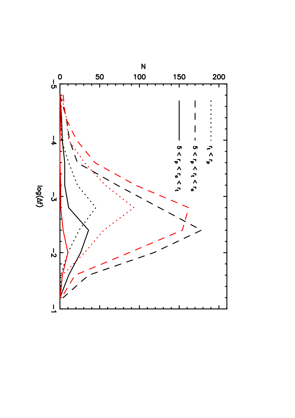
Figure 13 plots the distribution of for tube orbits of all types in models IA1 and LA1, separated into three groups by radial range: , , and , where and are the peri- and apocentre distances and is the radius at which the potential switches orientation. From Figure 3 we find for model IA1, whereas a similar measurement for LA1 gives . Orbits that never visit the inner region have low . Orbits that remain wholly within the inner region have higher diffusion rates, but they tend to be less numerous. Orbits that move across are the most abundant and have higher diffusivity in model IA1 than in LA1. It is this difference in the diffusion of tube orbits crossing the radius at which the potential reorients that we propose accounts for the different stability properties of models IA1 and LA1.