Matrix representations for 3D strain-gradient elasticity

Journal: Journal of the Mechanics and Physics of Solids

N. Auffray Email: Nicolas.auffray@univ-mlv.fr Corresponding author: Corresponding author Address: MSME, Université Paris-Est, Laboratoire Modélisation et Simulation Multi Echelle,MSME UMR 8208 CNRS, 5 bd Descartes, 77454 Marne-la-Vallée, France H. Le Quang Address: MSME, Université Paris-Est, Laboratoire Modélisation et Simulation Multi Echelle,MSME UMR 8208 CNRS, 5 bd Descartes, 77454 Marne-la-Vallée, France Q.C. He Email: qi-chang.he@univ-mlv.fr Corresponding author: Corresponding author Address: MSME, Université Paris-Est, Laboratoire Modélisation et Simulation Multi Echelle,MSME UMR 8208 CNRS, 5 bd Descartes, 77454 Marne-la-Vallée, France

Abstract

The theory of first strain gradient elasticity (SGE) is widely used to model size and non-local effects observed in materials and structures. For a material whose microstructure is centrosymmetric, SGE is characterized by a sixth-order elastic tensor in addition to the classical fourth-order elastic tensor. Even though the matrix form of the sixth-order elastic tensor is well-known in the isotropic case, its complete matrix representations seem to remain unavailable in the anisotropic cases. In the present paper, the explicit matrix representations of the sixth-order elastic tensor are derived and given for all the 3D anisotropic cases in a compact and well-structured way. These matrix representations are necessary to the development and application of SGE for anisotropic materials.

Keywords:

Strain gradient elasticity , Anisotropy , Higher order tensors

1 Introduction

In classical continuum mechanics (Truesdell and Toupin (1960); Truesdell and Noll (1965)), only the first displacement gradient is involved and all the higher order displacement gradients are neglected in measuring the deformations of a body. This usual kinematical framework turns out not to be rich enough to describe a variety of important mechanical and physical phenomena. In particular, the size effects and non-local behaviors due to the discrete nature of matter at a sufficiently small scale, the presence of microstructural defects or the existence of internal constraints cannot be captured by classical continuum mechanics (see, e.g., Marangantia and Sharma (2007) and the references cited therein for more details). The early development of high-order (or generalized) continuum theories of elasticity was undertaken in the 1960s and marked with the major contributions of Toupin (1962); Koiter (1964); Mindlin (1964); Mindlin (1965); Eringen (1968); Mindlin and Eshel (1968). For the last two decades, the development and application of high-order continuum theories have recently gained an impetus, owing to a growing interest in modeling and simulating size effects and non local behaviors observed in a variety of materials, such as polycrystalline materials, geomaterials, biomaterials and nanostructured materials, and in small size structures (see, e.g., Fleck and Hutchinson (1997); Nix and Gao (1998); Lam et al. (2003); dell’Isola et al. (2009); dell’Isola et al. (2011); Liu et al. (2011)). At the same time, the development of homogenization theories (see, e.g., Forest (1998); Kouznetsova et al. (2004); Trinh et al. (2012)) makes it possible to determine higher-order moduli in terms of material local properties and microstructure. In particular, it has been recently evidenced (Alibert et al. (2003); Seppecher et al. (2011)) that microstructures can be designed to render higher-grade effects predominant. From the numerical point of view, theories of generalized continua, such as strain-gradient theory, can be used to avoid explicitly meshing coarse heterogeneous materials (Kruch and Forest (1998); Tekoglu and Onck (2008); Pau and Trovalusci (2012)).

The theory of first strain-gradient elasticity (SGE) proposed by Mindlin (1964) and Mindlin and Eshel (1968) is among the most important high-order continuum theories which have been elaborated for the last half century, and it is currently widely used. In this theory, the infinitesimal strain tensor $\mathbf{\varepsilon}$ and its gradient $\mathbf{\omega}=\nabla\mathbf{\varepsilon}$ are linearly related to the second-order Cauchy stress tensor $\mathbf{\sigma}$ and the third-order hyperstress tensor $\mathbf{\tau}$ by equation (1) where a fourth-order tensor $\mathbb{C}$ , a fifth-order tensor $\mathbb{M}$ and a sixth-order tensor $\mathbb{A}$ are involved and verify the index permutation symmetry properties (2) and (3). The simplest one of these three tensors, $\mathbb{C}$ , defines the conventional elastic properties of a material. The study of $\mathbb{C}$ had experienced a long history (Love (1944)) before a complete understanding of $\mathbb{C}$ was achieved quite recently. In fact, only about 20 years ago and for the first time, Huo and Del Piero (1991) explicitly posed, rigorously formulated and treated the fundamental problem of determining all the rotational symmetry classes that the fourth-order elastic tensor $\mathbb{C}$ can possess. This problem has then received the attention of researchers from mechanics, materials science, physics, applied mathematics and engineering (see, e.g., Zheng and Boehler (1994); Forte and Vianello (1996); Forte and Vianello (1997); He and Zheng (1996); Xiao (1997); Chadwick et al. (2001); Bóna et al. (2004); Bóna et al. (2007); Moakher and Norris (2006)). A comprehensive understanding of $\mathbb{C}$ is now available in the sense that the correct answers to the following three fundamental questions have been provided:
(a) How many symmetry classes and which symmetry classes has $\mathbb{C}$ ?
(b) For every given symmetry class, how many independent material parameters has $\mathbb{C}$ ?
(c) For each given symmetry class, what is the explicit matrix form of $\mathbb{C}$ relative to an orthonormal basis ?
However, these questions remains largely open in regard to the fifth-order tensor $\mathbb{M}$ and sixth-order tensor $\mathbb{A}$ in the theory of SGE. Indeed, in the 3D isotropic situation, Toupin (1962) and Mindlin (1965) gave the general form of $\mathbb{A}$ containing 5 independent material parameters, and Mindlin (1964) showed that $\mathbb{M}$ must be zero. In the 2D context, Auffray et al. (2009a) derived all anisotropic matrices of $\mathbb{A}$ . At the present time, in the 3D case, few results are known. A first result was established by dell’Isola et al. (2009), they constructed and studied a matrix representation of the sixth-order tensor $\mathbb{A}$ in the isotropic situation. And, more recently, Papanicolopulos (2011) investigates features of the $\mathbb{M}$ tensor in the $\mathrm{SO(3)}$ -symmetry. For that symmetry class a coupling between the the gradient and the first gradient exists. But, apart from these results, little is known about $\mathbb{M}$ and $\mathbb{A}$ .

In developing and applying the theory of SGE, there is currently a real need for posing and answering the foregoing three questions about the fifth-order tensor $\mathbb{M}$ and sixth-order tensor $\mathbb{A}$ . We first consider materials whose microstructure is centro-symmetric. In this case, $\mathbb{M}$ becomes zero and investigations can be carried out only on $\mathbb{A}$ . In a companion paper dedicated to 3D SGE Le Quang et al. (2012), we have proved that $\mathbb{A}$ has 17 symmetry classes, identified the nature of each symmetry class and determined the number of independent material parameters of $\mathbb{A}$ belonging to a given symmetry class. Nevertheless, in the literature and in our aforementioned work, the 3D explicit matrix forms of $\mathbb{A}$ have not been furnished for the 16 anisotropic symmetry classes. This situation prevents the theory of first SGE from being developed and applied for anisotropic materials.

Compared with the classical fourth-order tensor $\mathbb{C}$ , the sixth-order tensor $\mathbb{A}$ is much more complex and richer. Indeed, $\mathbb{A}$ has $16$ anisotropic symmetry classes whereas $\mathbb{C}$ possesses $7$ ones. In this regard, remark that, for example, the transverse hemitropy and transverse isotropy are two distinct symmetry classes for $\mathbb{A}$ but shrink into one symmetry class for $\mathbb{C}$ . A similar phenomenon also occurs for the tetrahedral and cubic symmetries. In addition, even for the same symmetry class, the number of independent material parameters of $\mathbb{A}$ is much higher than that of $\mathbb{C}$ . For instance, the cubic symmetry, $\mathbb{C}$ contains $3$ independent parameters while $\mathbb{A}$ comprises $11$ ones.

The present work aims to solve the problem of obtaining the base of the explicit matrix representations of $\mathbb{A}$ for all the 17 symmetry classes. As will be seen, the complexity and richness of $\mathbb{A}$ make a proper solution to this problem not straightforward at all. In fact, even though the matrix form of $\mathbb{A}$ relative to an orthonormal basis is known, how to express $\mathbb{A}$ as a symmetric square matrix in a compact and well-structured way is far from being obvious.

The paper is organized as follows. In the next section, the constitutive law of SGE is recalled and the essential results obtained by Le Quang et al. (2012) about the symmetry classes of $\mathbb{A}$ are recapitulated together with the most important concepts involved. The main results obtained by the present work are given in section 3. They include the explicit matrix representations of $\mathbb{A}$ for the 17 symmetry classes, which are rendered very compact and well-structured by proposing an original three-to-one subscript correspondence. Each symmetry class is associated to a simple geometric figure, and the matrix representations of $\mathbb{A}$ are presented in such a manner that they can be directly used without resorting to the theory of rotational groups. In section 4, the logic of the three-to-one subscript correspondence chosen in section 3 is explained, the general structure of the matrix representations of $\mathbb{A}$ is highlighted, and some salient differences between first SGE and classical elasticity are emphasized. In section 5, a few concluding remarks are drawn.

2 Strain-gradient elasticity

2.1 Constitutive law

In the (first) strain-gradient theory of linear elasticity (see, e.g., Mindlin (1964); Mindlin and Eshel (1968)), the constitutive law gives the symmetric Cauchy stress tensor $\mathbf{\sigma}$ and the hyperstress tensor $\mathbf{\tau}$ in terms of the infinitesimal strain tensor $\mathbf{\varepsilon}$ and strain-gradient tensor $\mathbf{\omega}=\nabla\mathbf{\varepsilon}$ through the two linear relations:

\begin{cases}\sigma_{ij}=C_{ijlm}\varepsilon_{lm}+M_{ijlmn}\omega_{lmn},\\ \tau_{ijk}=M_{lmijk}\varepsilon_{lm}+A_{ijklmn}\omega_{lmn}.\end{cases}

(1)

Above, $\sigma_{ij}$ , $\varepsilon_{ij}$ , $\tau_{ijk}$ and $\omega_{ijk}=\varepsilon_{ij,k}$ are, respectively, the matrix components of $\mathbf{\sigma}$ , $\mathbf{\varepsilon}$ , $\mathbf{\tau}$ and $\nabla\mathbf{\varepsilon}$ relative to an orthonormal basis $\{\mathbf{e}_{1},\mathbf{e}_{2},\mathbf{e}_{2}\}$ of a three-dimensional (3D) Euclidean space; $C_{ijlm}$ , $M_{ijlmn}$ and $A_{ijklmn}$ are the matrix components of the fourth-, fifth- and sixth-order elastic stiffness tensors $\mathbb{C}$ , $\mathbb{M}$ and $\mathbb{A}$ , respectively. These matrix components have the following index permutation symmetry properties:

C_{ijlm}=C_{jilm}=C_{lmij}\text{, \ \ \ }M_{ijklm}=M_{jiklm}=M_{ijlkm},

(2)

A_{ijklmn}=A_{jiklmn}=A_{lmnijk}.

(3)

In the case where the microstructure of a material exhibits centro-symmetry, the fifth-order elastic stiffness tensor $\mathbb{M}$ of this material is null, so that the constitutive law (1) becomes uncoupled:

\begin{cases}\sigma_{ij}=C_{ijlm}\varepsilon_{lm},\\ \tau_{ijk}=A_{ijklmn}\omega_{lmn}.\end{cases}

(4)

In this paper, we are essentially interested in answering the question of what are the possible different matrix forms for $\mathbb{A}$ with the index symmetry property (3), referred to as the strain-gradient elasticity (SGE) tensor. The same question can be posed for $\mathbb{M}$ and will be treated in another paper.

2.2 Symmetry classes

In a recent paper (Le Quang et al. (2012)), we have solved the problem of determining all the symmetry classes that the sixth-order SGE tensor $\mathbb{A}$ can have. For the purpose of the present paper, we below recall some relevant definitions and summarize the main result obtained in Le Quang et al. (2012).

Let $\mathbf{Q}$ be an element of the 3D rotation group SO $(3)$ . An SGE tensor $\mathbb{A}$ is said to be invariant under the action of $\mathbf{Q}$ if

Q_{io}Q_{jp}Q_{kq}Q_{lr}Q_{ms}Q_{nt}A_{opqrst}=A_{ijklmn}.

(5)

The symmetry group of $\mathbb{A}$ is defined as the subgroup $\mathrm{G}_{\mathbb{A}}$ of $\mathrm{SO}(3)$ formed of all the 3D rotation tensors leaving $\mathbb{A}$ invariant:

\mathrm{G}_{\mathbb{A}}=\{\mathbf{Q}\in\mathrm{SO}(3)\left|Q_{io}Q_{jp}Q_{kq}Q_{lr}Q_{ms}Q_{nt}A_{opqrst}=A_{ijklmn}\right.\}\text{.}

(6)

From the physical point of view, it is meaningful to consider two SGE tensors $\mathbb{A}$ and $\mathbb{B}$ as exhibiting rotational symmetry of the same kind if their symmetry groups are conjugate in the sense that

\text{there exists a }\mathbf{Q\in}\text{ }\mathrm{SO}(3)\text{ such that }\mathrm{G}_{\mathrm{B}}=\mathbf{Q}\mathrm{G}_{\mathbb{A}}\mathbf{Q}^{T}.

(7)

Thus, the (rotational) symmetry class associated to an SGE tensor $\mathbb{A}$ can be naturally defined as the set $[\mathrm{G}_{\mathbb{A}}]$ of all the subgroups of SO $(3)$ conjugate to $\mathrm{G}_{\mathbb{A}}$ :

[\mathrm{G}_{\mathbb{A}}]=\{\mathrm{G}\subseteq\mathrm{SO}(3)\left|\mathrm{G}=\mathbf{Q}\mathrm{G}_{\mathbb{A}}\mathbf{Q}^{T},\mathbf{Q\in}\mathrm{SO}(3)\right.\}.

(8)

In other words, the symmetry class to which $\mathbb{A}$ belongs corresponds to its symmetry group modulo $\mathrm{SO}(3)$ . In fact, this classification leads to a partition of the set consisting of all the subgroups of $\mathrm{SO}(3)$ .

For later use, we introduce some additional notations. First, the rotation about a vector $\mathbf{a}$ through an angle $\theta\in[0,2\pi)$ is denoted by $\mathbf{Q}(\mathbf{a},\theta)$ ; in particular, the rotations $\mathbf{Q}(\mathbf{e}_{1}+\mathbf{e}_{2}+\mathbf{e}_{3},2\pi/3)$ and $\mathbf{Q}[2(\sqrt{5}-1)\mathbf{e}_{2}+(\sqrt{5}+1)\mathbf{e}_{3},2\pi/3]$ are in short noted as $\mathbf{\tilde{Q}}$ for $\mathbf{\hat{Q}}$ , respectively. In what follows, use will be made of the subsequent standard group notations: the second-order identity tensor group $\mathbf{I}$ ; the 2D rotation group $\mathrm{SO}(2)$ consisting of all rotations $\mathbf{Q}$ about a 3D vector, say $\mathbf{e}_{3}$ , such that $\mathbf{Q}\mathbf{e}_{3}=\mathbf{e}_{3}$ ; the 2D orthogonal group $O(2)$ composed of all orthogonal tensors $\mathbf{Q}$ such that $\mathbf{Q}\mathbf{e}_{3}=\pm\mathbf{e}_{3}$ for a fixed direction $\mathbf{e}_{3}$ ; the cyclic group $\mathrm{Z}_{r}$ with $r\geq 2$ elements generated by $\mathbf{Q}(\mathbf{e}_{3},2\pi/r)$ ; the dihedral group $\mathrm{D}_{r}$ $(r\geq 2)$ with $2r$ elements generated by $\mathbf{Q}(\mathbf{e}_{3},2\pi/r)$ and $\mathbf{Q}(\mathbf{e}_{1},\pi)$ ; the tetrahedral group $\mathcal{T}$ with 12 elements generated by $\mathrm{D}_{2}$ and $\mathbf{\tilde{Q}}$ ; the octahedral group $\mathcal{O}$ containing 24 elements generated by $\mathrm{D}_{4}$ and $\mathbf{\tilde{Q}}$ ; the icosahedral group $\mathcal{I}$ having 60 elements generated by $\mathrm{D}_{5}$ and $\mathbf{\hat{Q}}$ . Recall that the subgroups $\mathcal{T}$ , $\mathcal{O}$ and $\mathcal{I}$ map a tetrahedron, a cube and an icosahedron onto themselves, respectively.

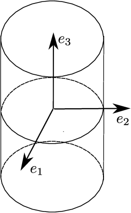
In the recent paper of Le Quang et al. (2012), it is proved that the number of all possible symmetry classes for the SGE tensors is $17$ . In addition, the number of independent matrix components of an SGE tensor belonging to a given symmetry class has also been determined by Le Quang et al. (2012). These results are summarized in Table 1 for the purpose of the present work. And all the 17 symmetry classes are graphically illustrated in Figures 1 to 17.

Name	Triclinic	Monoclinic	Orthotropic	Chirally trigonal	Trigonal
$[\mathrm{G}_{\mathbb{A}}]$	$\mathbf{I}$	$[\mathrm{Z}_{2}]$	$[\mathrm{D}_{2}]$	$[\mathrm{Z}_{3}]$	$[\mathrm{D}_{3}]$
$\#_{\mathrm{indep}}(\mathbb{A})$	$171$	$91$	$51$	$57$	$34$
Name	Chirally tetragonal	Tetragonal	Chirally pentagonal	Pentagonal	Chirally hexagonal
$[\mathrm{G}_{\mathbb{A}}]$	$[\mathrm{Z}_{4}]$	$[\mathrm{D}_{4}]$	$[\mathrm{Z}_{5}]$	[ $\mathrm{D}_{5}]$	$[\mathrm{Z}_{6}]$
$\#_{\mathrm{indep}}(\mathbb{A})$	$45$	$28$	$35$	$23$	$33$
Name	Hexagonal	Transversely hemitropic	Transversely isotropic	Tetrahedral	Cubic
$[\mathrm{G}_{\mathbb{A}}]$	$[\mathrm{D}_{6}]$	$[\mathrm{SO}(2)]$	$[\mathrm{O}(2)]$	$[\mathcal{T}]$	$[\mathcal{O}]$
$\#_{\mathrm{indep}}(\mathbb{A})$	$22$	$31$	$21$	$17$	$11$
Name	Icosahedral	Isotropic
$[\mathrm{G}_{\mathbb{A}}]$	$[\mathcal{I}]$	$\mathrm{SO}(3)$
$\#_{\mathrm{indep}}(\mathbb{A})$	$6$	$5$

Table 1: The names, the sets of subgroups

[\mathrm{G}_{\mathbb{A}}]

and the numbers of independent components

\#_{\mathrm{indep}}(\mathbb{A})

for the 17 symmetry classes of SGE.

Note that the number of all possible symmetry classes for the SGE tensors is much higher than the one for the classical elasticity tensors, since the former is $17$ while the latter is $8$ . In the totally anisotropic case where $[\mathrm{G}_{\mathbb{A}}]=\mathbf{I}$ and in the isotropic case where $[\mathrm{G}_{\mathbb{A}}]=\mathrm{SO}(3)$ , the number of independent components of $\mathbb{A}$ is equal to $171$ and $5$ , respectively. This clearly shows the SGE theory is much more complicated than the classical elasticity theory where the corresponding numbers are $21$ and $2$ , respectively.

3 Matrix representations of strain-gradient elasticity: main results

For an SGE tensor $\mathbb{A}$ belonging to one of the $17$ symmetry classes listed in Table 1, it is very important in various situations of theoretical and practical interest to know the explicit matrix form of $\mathbb{A}$ relative to an orthonormal basis $\{\mathbf{e}_{1},\mathbf{e}_{2},\mathbf{e}_{3}\}$ . To solve this problem in a satisfactory way, we need: (i) firstly to identify what are the non-zero matrix components of $\mathbb{A}$ and what are the possible relations between its non-zero components; (ii) secondly to elaborate an appropriate representation method according to which the matrix of $\mathbb{A}$ is well-structured and takes a simple and compact form so as to be used easily. The solution to the first part of the problem can be found in the paper of Le Quang et al. (2012). The solution to the second part of the problem is still lacking and will be provided in what follows.

3.1 Orthonormal basis and matrix component ordering

Let be defined the following subspace of third-order tensors

\mathcal{S}^{3}=\{\mathbb{T}|\mathbb{T}=\displaystyle\sum\limits_{i,j,k=1}^{3}T_{ijk}\mathbf{e}_{i}\otimes\mathbf{e}_{j}\otimes\mathbf{e}_{k},\text{ \ }T_{ijk}=T_{jik}\}

(9)

which is an 18-dimensional vector space. By (4), an SGE tensor $\mathbb{A}$ is a linear symmetric transformation from $\mathcal{S}^{3}$ to $\mathcal{S}^{3}$ . In order to express the strain gradient $\mathbf{\omega}$ or the hyperstress tensor $\mathbf{\tau}$ as a 18-dimensional vector and write $\mathbb{A}$ as a $18\times 18$ symmetric matrix, we introduce the following orthonormal basis vectors:

\mathbf{\hat{e}}_{\alpha}=\left(\frac{1-\delta_{ij}}{\sqrt{2}}+\frac{\delta_{ij}}{2}\right)\left(\mathbf{e}_{i}\otimes\mathbf{e}_{j}+\mathbf{e}_{j}\otimes\mathbf{e}_{i}\right)\otimes\mathbf{e}_{k},\quad 1\leq\alpha\leq 18

(10)

where the summation convention for a repeated subscript does not apply. Then, the strain gradient $\mathbf{\omega}$ , the hyperstress tensor $\mathbf{\tau}$ and the SGT $\mathbb{A}$ can be expressed as

\mathbf{\omega}=\displaystyle\sum\limits_{\alpha=1}^{18}\hat{\omega}_{\alpha}\mathbf{\hat{e}}_{\alpha},\text{ \ \ \ }\mathbf{\tau}=\displaystyle\sum\limits_{\alpha=1}^{18}\hat{\tau}_{\alpha}\mathbf{\hat{e}}_{\alpha},\text{ \ \ \ }\mathbb{A}=\displaystyle\sum\limits_{\alpha,\beta=1}^{18}\hat{A}_{\alpha\beta}\mathbf{\hat{e}}_{\alpha}\otimes\mathbf{\hat{e}}_{\beta},

(11)

so that the second SGE relation in (4) can be conveniently written in the matrix form

\hat{\tau}_{\alpha}=\hat{A}_{\alpha\beta}\hat{\omega}_{\beta}.

(12)

Note that, with the orthonormal basis (10), the relationship between the matrix components $\hat{\omega}_{\alpha}$ and $\omega_{ijk}$ , the one between $\hat{\tau}_{\alpha}$ and $\tau_{ijk}$ , and the one between $\hat{A}_{\alpha\beta}$ and $A_{ijklmn}$ are specified by

\hat{\omega}_{\alpha}=\begin{cases}\omega_{ijk}\text{ \ if \ }i=j,\\ \sqrt{2}\omega_{ijk}\text{ \ if \ }i\neq j;\end{cases}\text{ \ \ \ }\hat{\tau}_{\alpha}=\begin{cases}\tau_{ijk}\text{ \ if \ }i=j,\\ \sqrt{2}\tau_{ijk}\text{ \ if \ }i\neq j;\end{cases}

(13)

\hat{A}_{\alpha\beta}=\begin{cases}A_{ijklmn}\text{ \ if \ }i=j\ \text{and}\ l=m\text{,}\\ \sqrt{2}A_{ijklmn}\text{ \ if \ }i\neq j\ \text{and}\ l=m\ \text{or}\ i=j\ \text{and}\ l\neq m,\\ 2A_{ijklmn}\text{ \ if \ }i\neq j\ \text{and}\ l\neq m.\end{cases}

(14)

It remains to choose an appropriate three-to-one subscript correspondence between $ijk$ and $\alpha$ . For the SGE matrix $\hat{A}_{\alpha\beta}$ to be well-structured and exhibit a simple compact form for a given symmetry group $\mathrm{G}_{\mathbb{A}}$ , some criteria guiding the choice of an efficient three-to-one subscript correspondence are necessary. The criteria adopted in this work are detailed and explained in the next section. The final three-to-one subscript correspondence is specified in Table 2.

$\alpha$	$\mathbf{1}$	$\mathbf{2}$	$\mathbf{3}$	$4$	$5$
$ijk$	$\mathbf{111}$	$\mathbf{221}$	$\mathbf{122}$	$331$	$133$	Privileged direction: $1$
$\alpha$	$\mathbf{6}$	$\mathbf{7}$	$\mathbf{8}$	$9$	$10$
$ijk$	$\mathbf{222}$	$\mathbf{112}$	$\mathbf{121}$	$332$	$233$	Privileged direction: $2$
$\alpha$	$11$	$12$	$13$	$14$	$15$
$ijk$	$333$	$113$	$131$	$223$	$232$	Privileged direction: $3$
$\alpha$	$16$	$17$	$18$
$ijk$	$123$	$132$	$231$			No privileged direction

Table 2: The three-to-one subscript correspondence for 2D (in boldface in the table)and 3D strain-gradient elasticity

3.2 Rotation matrix

With the basis defined in (10) and the three-to-one subscript correspondence detailed in Table 2, the action of a rotation tensor $\mathbf{Q}\in\mathrm{SO}(3)$ on an SGE tensor $\mathbb{A}$ can be represented by a $18\times 18$ rotational matrix $\hat{Q}$ in such a way that

Q_{io}Q_{jp}Q_{kq}Q_{lr}Q_{ms}Q_{nt}A_{opqrst}=\hat{Q}_{\alpha\beta}\hat{A}_{\beta\gamma}\hat{Q}_{\gamma\delta}^{T}

(15)

where

\hat{Q}_{\alpha\beta}=\frac{1}{2}(Q_{io}Q_{jp}+Q_{ip}Q_{jo})Q_{kq}

(16)

with $\alpha$ and $\beta$ being associated to $ijk$ and $opq$ , respectively. Thus, formula (5) expressing the invariance of $\mathbb{A}$ under the action of $\mathbf{Q}$ is equivalent to

\hat{Q}\hat{A}\hat{Q}^{T}=\hat{A}

(17)

where $\hat{Q}$ stands for the $18\times 18$ matrix of components $\hat{Q}_{\alpha\beta}$ and $\hat{A}$ the $18\times 18$ matrix of components $\hat{A}_{\alpha\beta}$ .

3.3 Matrix representations for all symmetry classes

We are now ready to give the explicit expression of the SGE matrix $\hat{A}$ for each of the 17 symmetry classes. To be expressed in a simple and compact way, the matrix $\hat{A}$ for every symmetry class is split into sub-matrices so as to make appear elementary building blocks. The order adopted to specify the expressions of $\hat{A}$ for the symmetry classes $[\mathrm{Z}_{k}]$ and $[\mathrm{D}_{k}]$ is $k=1,$ $2,$ $4,$ $3,$ $6,$ $5$ and $\infty$ . The reason for such a choice is explained in subsection 4.2.

3.3.1 Symmetry class characterized by $\mathbf{I}$

Refer to caption — Figure 1: Triclinic system ( $\mathbf{I}$ -invariance): the material is completely asymmetric.

In this most general case, illustrated by figure 1, the material in question is totally anisotropic and the SGE matrix $\hat{A}$ comprises $171$ independent components. The explicit expression of $\hat{A}$ as a full $18\times 18$ symmetric matrix can be directly obtained by formula (14). We first define

1.

the $\frac{n(n+1)}{2}$ -dimensional space $\mathcal{M}^{S}(n)$ consisting of $n\times n$ symmetric matrices;
2.

the $n^{2}$ -dimensional space $\mathcal{M}(n)$ made of $n\times n$ matrices;
3.

the $nm$ -dimensional space $\mathcal{M}(n,m)$ composed of $n\times m$ matrices.

Then, we can write $\hat{A}$ in the following way

A_{\mathbf{I}}=\begin{pmatrix}\scriptstyle A^{(15)}&\scriptstyle B^{(25)}&\scriptstyle C^{(25)}&\scriptstyle D^{(15)}\\ &\scriptstyle E^{(15)}&\scriptstyle F^{(25)}&\scriptstyle G^{(15)}\\ &\scriptstyle&\scriptstyle H^{(15)}&\scriptstyle I^{(15)}\\ &\scriptstyle&\scriptstyle&\scriptstyle J^{(6)}\end{pmatrix}_{S}

where the subscript $S$ indicates that the matrix is symmetric and the form and number of independent components of each involved sub-matrix are specified by

1.

$A^{(15)},\ E^{(15)},\ H^{(15)}\in\mathcal{M}^{S}(5)$ ;
2.

$B^{(25)},\ C^{(25)},\ F^{(25)}\in\mathcal{M}(5)$ ;
3.

$D^{(15)},\ G^{(15)},\ I^{(15)}\in\mathcal{M}(5,3)$ ;
4.

$J^{(6)}\in\mathcal{M}^{S}(3)$ .

For example, $A^{(15)}$ is an element of $\mathcal{M}^{S}(5)$ and contains 15 independent components while $B^{(25)}$ belongs to $\mathcal{M}(5)$ and comprises 25 independent components.

3.3.2 Symmetry classes $[Z_{2}]$ and $[D_{2}]$

According as the symmetry class $[Z_{2}]$ or $[D_{2}]$ is concerned (c.f. figures 2 and 3), the material described is monoclinic or orthotropic, and the SGE matrix $\hat{A}$ contains $91$ or $51$ independent components. Using the three-to-one subscript correspondence given in Table 2, the SGE matrices exhibiting the $Z_{2}$ -symmetry and $D_{2}$ -symmetry are well-structured and take the compact forms:

A_{\mathrm{Z}^{\mathbf{e}_{3}}_{2}}=\begin{pmatrix}\scriptstyle A^{(15)}&\scriptstyle B^{(25)}&\scriptstyle 0&\scriptstyle 0\\ &\scriptstyle E^{(15)}&\scriptstyle 0&\scriptstyle 0\\ &\scriptstyle&\scriptstyle H^{(15)}&\scriptstyle I^{(15)}\\ &\scriptstyle&\scriptstyle&\scriptstyle J^{(6)}\end{pmatrix}_{S}\quad,\quad A_{\mathrm{Z}^{\mathbf{e}_{1}}_{2}}=\begin{pmatrix}\scriptstyle A^{(15)}&\scriptstyle 0&\scriptstyle 0&\scriptstyle D^{(15)}\\ &\scriptstyle E^{(15)}&\scriptstyle F^{(25)}&\scriptstyle 0\\ &\scriptstyle&\scriptstyle H^{(15)}&\scriptstyle 0\\ &\scriptstyle&\scriptstyle&\scriptstyle J^{(6)}\end{pmatrix}_{S}

A_{\mathrm{D}_{2}}=\begin{pmatrix}\scriptstyle A^{(15)}&\scriptstyle 0&\scriptstyle 0&\scriptstyle 0\\ &\scriptstyle E^{(15)}&\scriptstyle 0&\scriptstyle 0\\ &\scriptstyle&\scriptstyle H^{(15)}&\scriptstyle 0\\ &\scriptstyle&\scriptstyle&\scriptstyle J^{(6)}\end{pmatrix}_{S}

where $A^{(15)},\ E^{(15)},\ H^{(15)}\in\mathcal{M}^{S}(5)$ , $B^{(25)},F^{(25)}\in\mathcal{M}(5)$ , $I^{(15)},D^{(15)},\in\mathcal{M}(5,3)$ and $J^{(6)}\in\mathcal{M}^{S}(3)$ .

Here, because of its practical interest we give two conjugate representations of the same symmetry class $[Z_{2}]$ . In the first representation the $\pi$ -rotation is taken around $\mathbf{e}_{3}$ as indicated by the notation $\mathrm{Z}^{\mathbf{e}_{3}}_{2}$ , meanwhile in the second case the rotation is taken around $\mathbf{e}_{1}$ (as indicated by $\mathrm{Z}^{\mathbf{e}_{1}}_{2}$ ). The first situation is considered in order to be coherent with the representation of the other cyclic classes, in which the generating rotation is taken around $\mathbf{e}_{3}$ . The second representation we exhibit correspond to the common case of a monoclinic material, the combination of the $\mathrm{Z}^{\mathbf{e}_{1}}_{2}$ -invariance and the central inversion (always contained in the symmetry group of any even-order tensor) leads to the existence of symmetry plane which normal is $\mathbf{e}_{3}$ .

It is remarkable that the non-zero matrix blocks of $A_{\mathrm{D}_{2}}$ are diagonally located. Note that $A_{\mathrm{Z}^{\mathbf{e}_{1}}_{2}}$ and $A_{\mathrm{Z}^{\mathbf{e}_{3}}_{2}}$ are identical to $A_{\mathrm{D}_{2}}$ to within the two non-diagonal matrix blocks $B^{(25)}$ and $I^{(15)}$ , in one case and to within $E^{(25)}$ and $D^{(15)}$ in the other.

3.3.3 Symmetry classes $[Z_{4}]$ and $[D_{4}]$

The materials characterized by the symmetry classes $[D_{4}]$ and $[Z_{4}]$ , shown figures 4 and 5, are said to be tetragonal and chirally tetragonal. The numbers of independent components of $\hat{A}$ with the $D_{4}$ -symmetry and $Z_{4}$ -symmetry are $28$ and $45$ , respectively. To write the corresponding SGE matrices in a compact way, we first introduce

1.

the $\frac{n(n-1)}{2}$ -dimensional space $\mathcal{M}^{A}(n)$ consisting of $n\times n$ anti-symmetric matrices;
2.

the matrices $H^{(9)}$ , $I^{(7)}$ and $J^{(4)}$ with 9, 7 and 4 independent components defined by

H^{(9)}=\begin{pmatrix}\scriptstyle h_{11}&\scriptstyle h_{12}&\scriptstyle h_{13}&\scriptstyle h_{12}&\scriptstyle h_{13}\\ &\scriptstyle h_{22}&\scriptstyle h_{23}&\scriptstyle h_{24}&\scriptstyle h_{25}\\ &\scriptstyle&\scriptstyle h_{33}&\scriptstyle h_{25}&\scriptstyle h_{35}\\ &\scriptstyle&\scriptstyle&\scriptstyle h_{22}&\scriptstyle h_{23}\\ &\scriptstyle&\scriptstyle&\scriptstyle&\scriptstyle h_{33}\end{pmatrix}_{S}\quad,\quad I^{(7)}=\begin{pmatrix}\scriptstyle 0&\scriptstyle i_{12}&\scriptstyle-i_{12}\\ \scriptstyle i_{21}&\scriptstyle i_{22}&\scriptstyle i_{23}\\ \scriptstyle i_{31}&\scriptstyle i_{32}&\scriptstyle i_{33}\\ \scriptstyle-i_{21}&\scriptstyle-i_{23}&\scriptstyle-i_{22}\\ \scriptstyle-i_{31}&\scriptstyle-i_{33}&\scriptstyle-i_{32}\end{pmatrix}\quad,\quad J^{(4)}=\begin{pmatrix}\scriptstyle j_{11}&\scriptstyle j_{12}&\scriptstyle j_{12}\\ &\scriptstyle j_{22}&\scriptstyle j_{23}\\ &&\scriptstyle j_{22}\end{pmatrix}_{S}.

Then, the $Z_{4}$ -symmetric and $D_{4}$ -symmetric SGE matrices can be written as

A_{\mathrm{Z}_{4}}=\begin{pmatrix}\scriptstyle A^{(15)}&\scriptstyle B^{(10)}&\scriptstyle 0&\scriptstyle 0\\ &\scriptstyle A^{(15)}&\scriptstyle 0&\scriptstyle 0\\ &\scriptstyle&\scriptstyle H^{(9)}&\scriptstyle I^{(7)}\\ &\scriptstyle&\scriptstyle&\scriptstyle J^{(4)}\end{pmatrix}_{S}\quad,\quad A_{\mathrm{D}_{4}}=\begin{pmatrix}\scriptstyle A^{(15)}&\scriptstyle 0&\scriptstyle 0&\scriptstyle 0\\ &\scriptstyle A^{(15)}&\scriptstyle 0&\scriptstyle 0\\ &\scriptstyle&\scriptstyle H^{(9)}&\scriptstyle 0\\ &\scriptstyle&\scriptstyle&\scriptstyle J^{(4)}\end{pmatrix}_{S}

where $A^{(15)}\in\mathcal{M}^{S}(5)$ and $B^{(10)}\in\mathcal{M}^{A}(5)$ . Owing to the subscript ordering specified by Table 2, both the expressions of $A_{\mathrm{Z}_{4}}$ and $A_{\mathrm{D}_{4}}$ exhibit compact structure. In addition, $A_{\mathrm{D}_{4}}$ has a diagonal block structure.

3.3.4 Symmetry classes $[Z_{3}]$ and $[D_{3}]$

The materials having the symmetry classes $[D_{3}]$ and $[Z_{3}]$ , shown figures 6 and 7, are referred to as being trigonal and chirally trigonal, respectively. The numbers of independent components contained in the corresponding matrices $A_{\mathrm{Z}_{3}}$ and $A_{\mathrm{D}_{3}}$ are $57$ and $34$ , respectively. As will be seen, even if use is made of the subscript ordering of Table 2, the matrix expressions of $A_{\mathrm{Z}_{3}}$ and $A_{\mathrm{D}_{3}}$ remain quite complex. However, it is possible to get a good understanding of the structures of $A_{\mathrm{Z}_{3}}$ and $A_{\mathrm{D}_{3}}$ by defining appropriate independent sub-matrix blocks and making appear dependent sub-matrix blocks. More precisely, $A_{\mathrm{Z}_{3}}$ and $A_{\mathrm{D}_{3}}$ can be expressed as

A_{\mathrm{Z}_{3}}=\begin{pmatrix}\scriptstyle A^{(11)}+\eta A_{c}&\scriptstyle B^{(6)}+\theta B_{c}&\scriptstyle\scriptstyle C^{(3)}&\scriptstyle D^{(4)}\\ &\scriptstyle A^{(11)}&\scriptstyle F^{(8)}&\scriptstyle G^{(9)}\\ &\scriptstyle&\scriptstyle H^{(6)}&\scriptstyle I^{(4)}\\ &\scriptstyle&\scriptstyle&\scriptstyle J^{(4)}\end{pmatrix}_{S}+\begin{pmatrix}\scriptstyle 0&\scriptstyle 0&\scriptstyle\scriptstyle f(G^{(9)})&\scriptstyle f(F^{(8)})\\ &\scriptstyle 0&\scriptstyle f(D^{(4)})&\scriptstyle 0\\ &\scriptstyle&\scriptstyle f(J^{(4)})&\scriptstyle 0\\ &\scriptstyle&\scriptstyle&\scriptstyle 0\end{pmatrix}_{S},

A_{\mathrm{D}_{3}}=\begin{pmatrix}\scriptstyle A^{(11)}+\eta A_{c}&\scriptstyle 0&\scriptstyle 0&\scriptstyle D^{(4)}\\ &\scriptstyle A^{(11)}&\scriptstyle F^{(8)}&\scriptstyle 0\\ &\scriptstyle&\scriptstyle H^{(6)}&\scriptstyle 0\\ &\scriptstyle&\scriptstyle&\scriptstyle J^{(4)}\end{pmatrix}_{S}+\begin{pmatrix}\scriptstyle 0&\scriptstyle 0&\scriptstyle\scriptstyle 0&\scriptstyle f(F^{(8)})\\ &\scriptstyle 0&\scriptstyle f(D^{(4)})&\scriptstyle 0\\ &\scriptstyle&\scriptstyle f(J^{(4)})&\scriptstyle 0\\ &\scriptstyle&\scriptstyle&\scriptstyle 0\end{pmatrix}_{S}.

In these two expressions, $\eta$ and $\theta$ are two scalar material parameters; $A^{(11)}$ , $B^{(6)}$ , $C^{(3)}$ , $D^{(4)}$ , $F^{(8)}$ , $G^{(9)}$ , $H^{(6)}$ , $I^{(4)}$ and $J^{(4)}$ are 9 independent sub-matrices; $A_{c}$ and $B_{c}$ are two coupling matrices containing no material parameters; $f(G^{(9)})$ , $f(F^{(8)})$ , $f(D^{(4)})$ and $f(J^{(4)})$ are the matrix-value functions of $G^{(9)}$ , $F^{(8)}$ , $D^{(4)}$ and $J^{(4)}$ , respectively.

First, the expression of $A^{(11)}$ with 11 independent components is specified by

A^{(11)}=\begin{pmatrix}\scriptstyle a_{11}&\scriptstyle a_{12}&\scriptstyle a_{13}&\scriptstyle a_{14}&\scriptstyle a_{15}\\ &\scriptstyle a_{22}&\scriptstyle-a_{13}+\sqrt{2}\alpha_{\mathrm{III}}&\scriptstyle\alpha_{\mathrm{I}}&\scriptstyle\alpha_{\mathrm{II}}\\ &&\scriptstyle-a_{12}+\alpha_{\mathrm{III}}^{\star}&\scriptstyle a_{34}&\scriptstyle a_{35}\\ &&&\scriptstyle a_{44}&\scriptstyle a_{45}\\ &&&&\scriptstyle a_{55}\end{pmatrix}_{S}\ ,

where

\alpha_{\mathrm{I}}=a_{14}-\sqrt{2}a_{34}\ ,\ \alpha_{\mathrm{II}}=a_{15}-\sqrt{2}a_{35}\ ,\ \alpha_{\mathrm{III}}=\frac{a_{11}-a_{22}}{2}\ ,\ \alpha_{\mathrm{III}}^{\star}=\frac{a_{11}+a_{22}}{2}.

Next, the expressions of $B^{(6)}$ , $C^{(3)}$ , $D^{(4)}$ , $G^{(9)}$ , $H^{(6)}$ and $I^{(4)}$ are given by

B^{(6)}=\begin{pmatrix}\scriptstyle 0&\scriptstyle b_{12}&\scriptstyle-\frac{\sqrt{2}}{2}b_{12}&\scriptstyle b_{24}+\sqrt{2}b_{34}&\scriptstyle b_{25}+\sqrt{2}b_{35}\\ &\scriptstyle 0&\scriptstyle-\frac{\sqrt{2}}{2}b_{12}&\scriptstyle b_{24}&\scriptstyle b_{25}\\ &&\scriptstyle 0&\scriptstyle b_{34}&\scriptstyle b_{35}\\ &&&\scriptstyle 0&\scriptstyle b_{45}\\ &&&&\scriptstyle 0\end{pmatrix}_{A}\ ,

C^{(3)}=\begin{pmatrix}\scriptstyle c_{11}&\scriptstyle c_{12}&\scriptstyle c_{13}&\scriptstyle c_{12}&\scriptstyle c_{13}\\ -\scriptstyle c_{11}&\scriptstyle-c_{12}&\scriptstyle-c_{13}&\scriptstyle-c_{12}&\scriptstyle-c_{13}\\ \scriptstyle-\sqrt{2}c_{11}&\scriptstyle-\sqrt{2}c_{12}&\scriptstyle-\sqrt{2}c_{13}&\scriptstyle-\sqrt{2}c_{12}&\scriptstyle-\sqrt{2}c_{13}\\ \scriptstyle 0&\scriptstyle 0&\scriptstyle 0&\scriptstyle 0&\scriptstyle 0\\ \scriptstyle 0&\scriptstyle 0&\scriptstyle 0&\scriptstyle 0&\scriptstyle 0\end{pmatrix}\ ,\ D^{(4)}=\begin{pmatrix}\scriptstyle d_{11}&\scriptstyle d_{12}&\scriptstyle-d_{12}\\ \scriptstyle d_{11}&\scriptstyle-d_{12}&\scriptstyle d_{12}\\ \scriptstyle 0&\scriptstyle-\sqrt{2}d_{12}&\scriptstyle\sqrt{2}d_{12}\\ \scriptstyle d_{41}&\scriptstyle 0&\scriptstyle 0\\ \scriptstyle d_{51}&\scriptstyle 0&\scriptstyle 0\end{pmatrix},

F^{(8)}=\begin{pmatrix}\scriptstyle f_{11}&\scriptstyle f_{12}&\scriptstyle f_{13}&\scriptstyle f_{14}&\scriptstyle f_{15}\\ \scriptstyle-f_{11}&\scriptstyle-f_{12}+\beta_{\mathrm{I}}&\scriptstyle f_{23}&\scriptstyle-f_{12}+\beta_{\mathrm{I}}&\scriptstyle-f_{15}-2\beta_{\mathrm{II}}\\ \scriptstyle-\sqrt{2}f_{11}&\scriptstyle-\sqrt{2}(f_{12}-\frac{3\beta_{\mathrm{I}}}{2})&\scriptstyle-\sqrt{2}(f_{15}+\beta_{\mathrm{II}})&\scriptstyle-\sqrt{2}(f_{12}-\frac{\beta_{\mathrm{I}}}{2})&\scriptstyle-\sqrt{2}(f_{13}-\beta_{\mathrm{II}})\\ \scriptstyle 0&\scriptstyle 0&\scriptstyle f_{43}&\scriptstyle 0&\scriptstyle-f_{43}\\ \scriptstyle 0&\scriptstyle 0&\scriptstyle f_{53}&\scriptstyle 0&\scriptstyle-f_{53}\\ &&&&\end{pmatrix}

with

\beta_{\mathrm{I}}=\frac{f_{12}-f_{14}}{2}\quad,\quad\beta_{\mathrm{II}}=\frac{f_{13}+f_{23}}{2},

G^{(9)}=\begin{pmatrix}\scriptstyle g_{11}&\scriptstyle g_{12}&\scriptstyle g_{13}\\ \scriptstyle g_{21}&\scriptstyle g_{23}-2\gamma_{\mathrm{III}}&\scriptstyle g_{23}\\ \scriptstyle\sqrt{2}\gamma_{\mathrm{I}}&\scriptstyle\sqrt{2}\gamma_{\mathrm{II}}&\scriptstyle\sqrt{2}(2\gamma_{\mathrm{III}}+\gamma_{\mathrm{II}})\\ \scriptstyle g_{41}&\scriptstyle g_{42}&\scriptstyle g_{42}\\ \scriptstyle g_{51}&\scriptstyle g_{52}&\scriptstyle g_{52}\end{pmatrix}

with

\gamma_{\mathrm{I}}=\frac{g_{11}-g_{21}}{2}\quad,\quad\gamma_{\mathrm{II}}=\frac{g_{13}-g_{23}}{2}\quad,\quad\gamma_{\mathrm{III}}=\frac{g_{12}-g_{13}}{2},

H^{(6)}=\begin{pmatrix}\scriptstyle h_{11}&\scriptstyle h_{12}&\scriptstyle h_{13}&\scriptstyle h_{12}&\scriptstyle h_{13}\\ &\scriptstyle h_{22}&\scriptstyle h_{23}&\scriptstyle h_{22}&\scriptstyle h_{23}\\ &\scriptstyle&\scriptstyle h_{33}&\scriptstyle h_{23}&\scriptstyle h_{33}\\ &\scriptstyle&\scriptstyle&\scriptstyle h_{22}&\scriptstyle h_{23}\\ &\scriptstyle&\scriptstyle&\scriptstyle&\scriptstyle h_{33}\end{pmatrix}_{S}\ ,\ I^{(4)}=\begin{pmatrix}\scriptstyle 0&\scriptstyle i_{12}&\scriptstyle-i_{12}\\ \scriptstyle 0&\scriptstyle i_{22}&\scriptstyle-i_{22}-\sqrt{2}i_{31}\\ \scriptstyle i_{31}&\scriptstyle i_{32}&\scriptstyle-i_{32}\\ \scriptstyle 0&\scriptstyle i_{22}+\sqrt{2}i_{31}&\scriptstyle-i_{22}\\ \scriptstyle-i_{31}&\scriptstyle i_{32}&\scriptstyle-i_{32}\end{pmatrix}.

The matrices $A_{c}$ and $B_{c}$ are independent of material parameters and take the following forms:

A_{c}=\begin{pmatrix}\scriptstyle 1&\scriptstyle-1&\scriptstyle-\sqrt{2}&\scriptstyle 0&\scriptstyle 0\\ &\scriptstyle 1&\scriptstyle\sqrt{2}&\scriptstyle 0&\scriptstyle 0\\ &\scriptstyle&\scriptstyle 2&\scriptstyle 0&\scriptstyle 0\\ &\scriptstyle&\scriptstyle&\scriptstyle 0&\scriptstyle 0\\ &\scriptstyle&\scriptstyle&\scriptstyle&\scriptstyle 0\end{pmatrix}_{S}\text{ ,}

B_{c}=\begin{pmatrix}\scriptstyle 1&\scriptstyle 0&\scriptstyle-\frac{3\sqrt{2}}{2}&\scriptstyle 0&\scriptstyle 0\\ \scriptstyle-2&\scriptstyle 1&\scriptstyle\frac{\sqrt{2}}{2}&\scriptstyle 0&\scriptstyle 0\\ \scriptstyle-\frac{\sqrt{2}}{2}&\scriptstyle\frac{3\sqrt{2}}{2}&\scriptstyle 2&\scriptstyle 0&\scriptstyle 0\\ \scriptstyle 0&\scriptstyle 0&\scriptstyle 0&\scriptstyle 0&\scriptstyle 0\\ \scriptstyle 0&\scriptstyle 0&\scriptstyle 0&\scriptstyle 0&\scriptstyle 0\end{pmatrix}\text{ .}

Finally, the matrix-value functions $f(G^{(9)})$ , $f(F^{(8)})$ , $f(D^{(4)})$ and $f(J^{(4)})$ are defined by

f(G^{(9)})=\begin{pmatrix}\scriptstyle 0&\scriptstyle-\frac{\sqrt{2}}{2}\gamma_{\mathrm{I}}^{\star}&\scriptstyle-g_{12}-\gamma_{\mathrm{II}}&\scriptstyle\frac{\sqrt{2}}{2}(g_{11}+\gamma_{\mathrm{I}})&\scriptstyle\gamma_{\mathrm{II}}^{\star}\\ \scriptstyle 0&\scriptstyle-\frac{\sqrt{2}}{2}\gamma_{\mathrm{I}}^{\star}&\scriptstyle-g_{12}+3\gamma_{\mathrm{II}}+4\gamma_{\mathrm{III}}&\scriptstyle\frac{\sqrt{2}}{2}(g_{11}+\gamma_{\mathrm{I}})&\scriptstyle\gamma_{\mathrm{II}}^{\star}\\ \scriptstyle 0&\scriptstyle-2\gamma_{\mathrm{I}}&\scriptstyle 0&\scriptstyle 0&\scriptstyle 2\sqrt{2}(\gamma_{\mathrm{III}}+\gamma_{\mathrm{II}})\\ \scriptstyle 0&\scriptstyle-\frac{\sqrt{2}}{2}g_{41}&\scriptstyle-g_{42}&\scriptstyle\frac{\sqrt{2}}{2}g_{41}&\scriptstyle g_{42}\\ \scriptstyle 0&\scriptstyle-\frac{\sqrt{2}}{2}g_{51}&\scriptstyle-g_{52}&\scriptstyle\frac{\sqrt{2}}{2}g_{51}&\scriptstyle g_{52}\end{pmatrix},

f(F^{(8)})=\begin{pmatrix}\scriptstyle\sqrt{2}\alpha&\scriptstyle\beta_{\mathrm{II}}&\scriptstyle-2\beta_{\mathrm{III}}-\beta_{\mathrm{II}}\\ \scriptstyle 0&\scriptstyle\beta_{\mathrm{II}}&\scriptstyle 3\beta_{\mathrm{II}}-2\beta_{\mathrm{III}}\\ \scriptstyle\alpha&\scriptstyle-2\sqrt{2}(\beta_{\mathrm{II}}-\beta_{\mathrm{III}})&\scriptstyle 0\\ \scriptstyle 0&\scriptstyle f_{43}&\scriptstyle f_{43}\\ \scriptstyle 0&\scriptstyle f_{53}&\scriptstyle f_{53}\end{pmatrix}

with

\gamma_{\mathrm{I}}^{\star}=\frac{g_{11}+g_{21}}{2}\quad,\quad\gamma_{\mathrm{II}}^{\star}=\frac{g_{13}+g_{23}}{2}\quad\text{and}\quad\beta_{\mathrm{III}}=\frac{f_{13}-f_{15}}{2},

f(D^{(4)})=\begin{pmatrix}\scriptstyle 0&\scriptstyle\frac{\sqrt{2}}{2}d_{11}&\scriptstyle 0&\scriptstyle-\frac{\sqrt{2}}{2}d_{11}&\scriptstyle 0\\ \scriptstyle 0&\scriptstyle\frac{\sqrt{2}}{2}d_{11}&\scriptstyle 0&\scriptstyle-\frac{\sqrt{2}}{2}d_{11}&\scriptstyle 0\\ \scriptstyle 0&\scriptstyle 0&\scriptstyle 0&\scriptstyle 0&\scriptstyle 0\\ \scriptstyle 0&\scriptstyle\frac{\sqrt{2}}{2}d_{41}&\scriptstyle 0&\scriptstyle-\frac{\sqrt{2}}{2}d_{41}&\scriptstyle 0\\ \scriptstyle 0&\scriptstyle\frac{\sqrt{2}}{2}d_{51}&\scriptstyle 0&\scriptstyle-\frac{\sqrt{2}}{2}d_{51}&\scriptstyle 0\end{pmatrix}\ ,\text{ }\ f(J^{(4)})=\begin{pmatrix}\scriptstyle 0&\scriptstyle 0&\scriptstyle 0&\scriptstyle 0&\scriptstyle 0\\ &\scriptstyle 0&\scriptstyle 0&\scriptstyle-j_{11}&\scriptstyle-\sqrt{2}j_{12}\\ &\scriptstyle&\scriptstyle 0&\scriptstyle-\sqrt{2}j_{12}&\scriptstyle-(j_{22}+j_{23})\\ &\scriptstyle&\scriptstyle&\scriptstyle 0&\scriptstyle 0\\ &\scriptstyle&\scriptstyle&\scriptstyle&\scriptstyle 0\end{pmatrix}_{S}

3.3.5 Symmetry classes $[Z_{6}]$ and $[D_{6}]$

The hexagonal and chirally hexagonal materials are described by the symmetry classes $[D_{6}]$ and $[Z_{6}]$ , illustrated by figures 8 and 9, and have $22$ and $33$ independent parameters, respectively. They can be considered as being degenerated from the trigonal and chirally trigonal materials. Precisely, the associated SGE matrices $A_{\mathrm{Z}_{6}}$ and $A_{\mathrm{D}_{6}}$ take the following simpler forms:

A_{\mathrm{Z}_{6}}=\begin{pmatrix}\scriptstyle A^{(11)}+\eta A_{c}&\scriptstyle B^{(6)}+\theta B_{c}&\scriptstyle 0&\scriptstyle 0\\ &\scriptstyle A^{(11)}&\scriptstyle 0&\scriptstyle 0\\ &\scriptstyle&\scriptstyle H^{(6)}&\scriptstyle I^{(4)}\\ &\scriptstyle&\scriptstyle&\scriptstyle J^{(4)}\end{pmatrix}_{S}+\begin{pmatrix}\scriptstyle 0&\scriptstyle 0&\scriptstyle 0&\scriptstyle 0\\ &\scriptstyle 0&\scriptstyle 0&\scriptstyle 0\\ &\scriptstyle&\scriptstyle f(J^{(4)})&\scriptstyle 0\\ &\scriptstyle&\scriptstyle&\scriptstyle 0\end{pmatrix}_{S}\text{ ,}

A_{\mathrm{D}_{6}}=\begin{pmatrix}\scriptstyle A^{(11)}+\eta A_{c}&\scriptstyle 0&\scriptstyle 0&\scriptstyle 0\\ &\scriptstyle A^{(11)}&\scriptstyle 0&\scriptstyle 0\\ &\scriptstyle&\scriptstyle H^{(6)}&\scriptstyle 0\\ &\scriptstyle&\scriptstyle&\scriptstyle J^{(4)}\end{pmatrix}_{S}+\begin{pmatrix}\scriptstyle 0&\scriptstyle 0&\scriptstyle 0&\scriptstyle 0\\ &\scriptstyle 0&\scriptstyle 0&\scriptstyle 0\\ &\scriptstyle&\scriptstyle f(J^{(4)})&\scriptstyle 0\\ &\scriptstyle&\scriptstyle&\scriptstyle 0\end{pmatrix}_{S}\text{ }

where $\eta$ and $\theta$ are two scalar parameters and the non-zero matrix blocks are identical to the relevant ones given for the symmetry class $[Z_{3}]$ .

3.3.6 Symmetry classes $[Z_{5}]$ and $[D_{5}]$ .

According as a material belongs to the pentagonal symmetry class $[D_{5}]$ or chirally pentagonal symmetry $[Z_{5}]$ , its number of independent parameters is $23$ or $35$ . The corresponding SGE matrices (see figures 10 and 11) $A_{\mathrm{Z}_{5}}$ and $A_{\mathrm{D}_{5}}$ are given by

A_{\mathrm{Z}_{5}}=\begin{pmatrix}\scriptstyle A^{(11)}&\scriptstyle B^{(6)}&\scriptstyle 0&\scriptstyle 0\\ &\scriptstyle A^{(11)}&\scriptstyle F^{(2)}&\scriptstyle G^{(2)}\\ &\scriptstyle&\scriptstyle H^{(6)}&\scriptstyle I^{(4)}\\ &\scriptstyle&\scriptstyle&\scriptstyle J^{(4)}\end{pmatrix}_{S}+\begin{pmatrix}\scriptstyle 0&\scriptstyle 0&\scriptstyle\scriptstyle f(G^{(2)})&\scriptstyle f(F^{(2)})\\ &\scriptstyle 0&\scriptstyle 0&\scriptstyle 0\\ &\scriptstyle&\scriptstyle g(J^{(4)})&\scriptstyle 0\\ &\scriptstyle&\scriptstyle&\scriptstyle 0\end{pmatrix}_{S},

A_{\mathrm{D}_{5}}=\begin{pmatrix}\scriptstyle A^{(11)}&\scriptstyle 0&\scriptstyle 0&\scriptstyle 0\\ &\scriptstyle A^{(11)}&\scriptstyle F^{(2)}&\scriptstyle 0\\ &\scriptstyle&\scriptstyle H^{(6)}&\scriptstyle 0\\ &\scriptstyle&\scriptstyle&\scriptstyle J^{(4)}\end{pmatrix}_{S}+\begin{pmatrix}\scriptstyle 0&\scriptstyle 0&\scriptstyle\scriptstyle 0&\scriptstyle f(F^{(2)})\\ &\scriptstyle 0&\scriptstyle 0&\scriptstyle 0\\ &\scriptstyle&\scriptstyle f(J^{(4)})&\scriptstyle 0\\ &\scriptstyle&\scriptstyle&\scriptstyle 0\end{pmatrix}_{S}.

In these two expressions, the sub-matrices $A^{(11)}$ , $B^{(6)}$ , $H^{(6)}$ , $I^{(4)}$ and $J^{(4)}$ are specified in the foregoing case where the trigonal and chirally trigonal symmetry classes, $[\mathrm{D}_{3}]$ and $[\mathrm{Z}_{3}]$ , are concerned. The remaining sub-matrices $F^{(2)}$ and $G^{(2)}$ , each of which contains 2 independent components, and the matrix-value functions $f(F^{(2)})$ , $f(G^{(2)})$ and $g(J^{(4)})$ take the followings forms:

F^{(2)}=\begin{pmatrix}\scriptstyle 0&\scriptstyle f_{12}&\scriptstyle f_{13}&\scriptstyle-f_{12}&\scriptstyle-f_{13}\\ \scriptstyle 0&\scriptstyle-f_{12}&\scriptstyle-f_{13}&\scriptstyle f_{12}&\scriptstyle f_{13}\\ \scriptstyle 0&\scriptstyle-\sqrt{2}f_{12}&\scriptstyle-\sqrt{2}f_{13}&\scriptstyle\sqrt{2}f_{12}&\scriptstyle\sqrt{2}f_{13}\\ \scriptstyle 0&\scriptstyle 0&\scriptstyle 0&\scriptstyle 0&\scriptstyle 0\\ \scriptstyle 0&\scriptstyle 0&\scriptstyle 0&\scriptstyle 0&\scriptstyle 0\end{pmatrix}\ ,\ \ G^{(2)}=\begin{pmatrix}\scriptstyle g_{11}&\scriptstyle g_{12}&\scriptstyle g_{12}\\ \scriptstyle-g_{11}&\scriptstyle-g_{12}&\scriptstyle-g_{12}\\ \scriptstyle-\sqrt{2}g_{11}&\scriptstyle-\sqrt{2}g_{12}&\scriptstyle-\sqrt{2}g_{12}\\ \scriptstyle 0&\scriptstyle 0&\scriptstyle 0\\ \scriptstyle 0&\scriptstyle 0&\scriptstyle 0\end{pmatrix},

f(F^{(2)})=\begin{pmatrix}\scriptstyle-\sqrt{2}f_{12}&\scriptstyle-f_{13}&\scriptstyle-f_{13}\\ \scriptstyle\sqrt{2}f_{12}&\scriptstyle f_{13}&\scriptstyle f_{13}\\ \scriptstyle 2f_{12}&\scriptstyle\sqrt{2}f_{13}&\scriptstyle\sqrt{2}f_{13}\\ \scriptstyle 0&\scriptstyle 0&\scriptstyle 0\\ \scriptstyle 0&\scriptstyle 0&\scriptstyle 0\end{pmatrix}\ ,\ \ f(G^{(2)})=\begin{pmatrix}\scriptstyle 0&\scriptstyle\frac{\sqrt{2}}{2}g_{11}&\scriptstyle g_{12}&\scriptstyle-\frac{\sqrt{2}}{2}g_{11}&-\scriptstyle g_{12}\\ \scriptstyle 0&\scriptstyle-\frac{\sqrt{2}}{2}g_{11}&-\scriptstyle g_{12}&\scriptstyle\frac{\sqrt{2}}{2}g_{11}&\scriptstyle g_{12}\\ \scriptstyle 0&\scriptstyle-g_{11}&\scriptstyle-\sqrt{2}g_{12}&\scriptstyle g_{11}&\scriptstyle\sqrt{2}g_{12}\\ \scriptstyle 0&\scriptstyle 0&\scriptstyle 0&\scriptstyle 0&\scriptstyle 0\\ \scriptstyle 0&\scriptstyle 0&\scriptstyle 0&\scriptstyle 0&\scriptstyle 0\end{pmatrix},

g(J^{(4)})=\begin{pmatrix}\scriptstyle 0&\scriptstyle 0&\scriptstyle 0&\scriptstyle 0&\scriptstyle 0\\ &\scriptstyle 0&\scriptstyle\sqrt{2}j_{12}&\scriptstyle-j_{11}&\scriptstyle 0\\ &\scriptstyle&\scriptstyle 0&\scriptstyle 0&\scriptstyle-(j_{22}+j_{23})\\ &\scriptstyle&\scriptstyle&\scriptstyle 0&\scriptstyle\sqrt{2}j_{12}\\ &\scriptstyle&\scriptstyle&\scriptstyle&\scriptstyle 0\end{pmatrix}_{S}\text{ .}

3.3.7 Symmetry classes $[\mathrm{SO}(2)]$ and $[\mathrm{O}(2)]$ .

These two symmetry classes, shown by figures 12 and 13, characterize the transversely hemitropic and transversely isotropic materials, respectively. The associated SGE matrices $A_{\mathrm{SO}(2)}$ and $A_{\mathrm{O}(2)}$ , containing $31$ and $21$ independent components, respectively, have the following expressions:

A_{\mathrm{SO}(2)}=\begin{pmatrix}\scriptstyle A^{(11)}&\scriptstyle B^{(6)}&\scriptstyle 0&\scriptstyle 0\\ &\scriptstyle A^{(11)}&\scriptstyle 0&\scriptstyle 0\\ &\scriptstyle&\scriptstyle H^{(6)}&\scriptstyle I^{(4)}\\ &\scriptstyle&\scriptstyle&\scriptstyle J^{(4)}\end{pmatrix}_{S}+\begin{pmatrix}\scriptstyle 0&\scriptstyle 0&\scriptstyle\scriptstyle 0&\scriptstyle 0\\ &\scriptstyle 0&\scriptstyle 0&\scriptstyle 0\\ &\scriptstyle&\scriptstyle f(J^{(4)})&\scriptstyle 0\\ &\scriptstyle&\scriptstyle&\scriptstyle 0\end{pmatrix}_{S}\text{ ,}

A_{\mathrm{O}(2)}=\begin{pmatrix}\scriptstyle A^{(11)}&\scriptstyle 0&\scriptstyle 0&\scriptstyle 0\\ &\scriptstyle A^{(11)}&\scriptstyle 0&\scriptstyle 0\\ &\scriptstyle&\scriptstyle H^{(6)}&\scriptstyle 0\\ &\scriptstyle&\scriptstyle&\scriptstyle J^{(4)}\end{pmatrix}_{S}+\begin{pmatrix}\scriptstyle 0&\scriptstyle 0&\scriptstyle\scriptstyle 0&\scriptstyle 0\\ &\scriptstyle 0&\scriptstyle 0&\scriptstyle 0\\ &\scriptstyle&\scriptstyle f(J^{(4)})&\scriptstyle 0\\ &\scriptstyle&\scriptstyle&\scriptstyle 0\end{pmatrix}_{S}\text{ ,}

where the sub-matrices $A^{(11)}$ , $B^{(6)}$ , $H^{(6)}$ , $I^{(4)}$ and $J^{(4)}$ are defined in studying the trigonal and chirally trigonal symmetry classes $[\mathrm{D}_{3}]$ and $[\mathrm{Z}_{3}]$ .

3.3.8 Symmetry classes $[\mathcal{T}]$ and $[\mathcal{O}]$ .

The materials described by the symmetry classes $[\mathcal{T}]$ and $[\mathcal{O}]$ shown by figures 14 and 15, are said to be tetrahedral and cubic, respectively. The former is characterized by 17 independent material parameters and the latter by 11 ones. The corresponding SGE matrices $A_{\mathcal{T}}$ and $A_{\mathcal{O}}$ have the expressions:

A_{\mathcal{T}}=\begin{pmatrix}\scriptstyle A^{(15)}&\scriptstyle 0&\scriptstyle 0&\scriptstyle 0\\ &\scriptstyle PA^{(15)}P^{T}&\scriptstyle 0&\scriptstyle 0\\ &\scriptstyle&\scriptstyle A^{(15)}&\scriptstyle 0\\ &\scriptstyle&\scriptstyle&\scriptstyle J^{(2)}\end{pmatrix}_{S}\text{ },\quad A_{\mathcal{O}}=\begin{pmatrix}\scriptstyle A^{(9)}&\scriptstyle 0&\scriptstyle 0&\scriptstyle 0\\ &\scriptstyle A^{(9)}&\scriptstyle 0&\scriptstyle 0\\ &\scriptstyle&\scriptstyle A^{(9)}&\scriptstyle 0\\ &\scriptstyle&\scriptstyle&\scriptstyle J^{(2)}\end{pmatrix}_{S},

where $A^{(15)}$ is an element of $\mathcal{M}^{S}(5)$ , $P$ is the permutation matrix defined by

P=\begin{pmatrix}1&0&0&0&0\\ 0&0&0&1&0\\ 0&0&0&0&1\\ 0&1&0&0&0\\ 0&0&1&0&0\end{pmatrix},

and the sub-matrices $A^{(9)}$ and $J^{(2)}$ , with 9 and 2 independent material parameters, are specified by

A^{(9)}=\begin{pmatrix}\scriptstyle a_{11}&\scriptstyle a_{12}&\scriptstyle a_{13}&\scriptstyle a_{12}&\scriptstyle a_{13}\\ &\scriptstyle a_{22}&\scriptstyle a_{23}&\scriptstyle a_{24}&\scriptstyle a_{25}\\ &\scriptstyle&\scriptstyle a_{33}&\scriptstyle a_{25}&\scriptstyle a_{35}\\ &\scriptstyle&\scriptstyle&\scriptstyle a_{22}&\scriptstyle a_{23}\\ &\scriptstyle&\scriptstyle&\scriptstyle&\scriptstyle a_{33}\end{pmatrix}_{S}\ ,\ \ J^{(2)}=\begin{pmatrix}\scriptstyle j_{11}&\scriptstyle j_{12}&\scriptstyle j_{12}\\ &\scriptstyle j_{11}&\scriptstyle j_{12}\\ &&\scriptstyle j_{11}\end{pmatrix}_{S}\text{ .}

Note that both $A_{\mathcal{T}}$ and $A_{\mathcal{O}}$ have a very compact diagonal structure.

3.3.9 Symmetry classes $[\mathcal{I}]$ and $[\mathrm{SO}(3)]$

The last symmetry classes $[\mathcal{I}]$ and $[\mathrm{SO}(3)]$ shown by figures 15 and 16, are icosahedral and isotropic. The corresponding SGE matrices $A_{\mathcal{I}}$ and $A_{\mathrm{SO}(3)}$ comprises 6 and 5 independent material parameters, respectively. They have the following expressions:

A_{\mathcal{I}}=\begin{pmatrix}\scriptstyle A^{(5)}+\eta A_{\mathcal{I}}^{(c)}&\scriptstyle 0&\scriptstyle 0&\scriptstyle 0\\ &\scriptstyle P(A^{(5)}+\eta A_{\mathcal{I}}^{(c)})P^{T}&\scriptstyle 0&\scriptstyle 0\\ &\scriptstyle&\scriptstyle A^{(5)}+\eta A_{\mathcal{I}}^{(c)}&\scriptstyle 0\\ &\scriptstyle&\scriptstyle&\scriptstyle\eta J_{c}\end{pmatrix}_{S}+\begin{pmatrix}\scriptstyle 0&\scriptstyle 0&\scriptstyle 0&\scriptstyle 0\\ &\scriptstyle 0&\scriptstyle 0&\scriptstyle 0\\ &\scriptstyle&\scriptstyle 0&\scriptstyle 0\\ &\scriptstyle&\scriptstyle&\scriptstyle f(A^{(5)})\end{pmatrix}_{S}\text{ ,}

A_{\mathrm{SO}(3)}=\begin{pmatrix}\scriptstyle A^{(5)}&\scriptstyle 0&\scriptstyle 0&\scriptstyle 0\\ &\scriptstyle A^{(5)}&\scriptstyle 0&\scriptstyle 0\\ &\scriptstyle&\scriptstyle A^{(5)}&\scriptstyle 0\\ &\scriptstyle&\scriptstyle&\scriptstyle 0\end{pmatrix}_{S}+\begin{pmatrix}\scriptstyle 0&\scriptstyle 0&\scriptstyle 0&\scriptstyle 0\\ &\scriptstyle 0&\scriptstyle 0&\scriptstyle 0\\ &\scriptstyle&\scriptstyle 0&\scriptstyle 0\\ &\scriptstyle&\scriptstyle&\scriptstyle f(A^{(5)})\end{pmatrix}_{S}\text{ ,}

where $\eta$ is a scalar material parameter, the $5\times 5$ sub-matrix $A^{(5)}$ contains 5 independent material parameters, $P$ is the same permutation matrix as the one defined in treating the tetrahedral symmetry class $[\mathcal{T}]$ , $A_{\mathcal{I}}^{(c)}$ is a $5\times 5$ sub-matrix containing no material parameter, $J_{c}$ is a $3\times 5$ sub-matrix involving the the golden number and $f(A^{(5)})$ is a matrix-value function of $A^{(5)}$ .

More precisely, $A^{(5)}$ takes the form

A^{(5)}=\begin{pmatrix}\scriptstyle a_{11}&\scriptstyle a_{12}&\scriptstyle a_{13}&\scriptstyle a_{12}&\scriptstyle a_{13}\\ &\scriptstyle a_{22}&\scriptstyle-a_{13}+\sqrt{2}\alpha_{\mathrm{III}}&\scriptstyle a_{12}-\sqrt{2}\alpha_{\mathrm{IV}}^{\star}&\scriptstyle\alpha_{\mathrm{IV}}^{\star}\\ &\scriptstyle&\scriptstyle-a_{12}+\alpha_{\mathrm{IV}}&\scriptstyle\alpha_{\mathrm{IV}}^{\star}&\scriptstyle a_{35}\\ &\scriptstyle&\scriptstyle&\scriptstyle a_{22}&\scriptstyle-a_{13}+\sqrt{2}\alpha_{\mathrm{III}}\\ &\scriptstyle&\scriptstyle&\scriptstyle&\scriptstyle-a_{12}+\alpha_{\mathrm{IV}}\end{pmatrix}_{S}

with

\alpha_{\mathrm{III}}=\frac{a_{11}-a_{22}}{2}\ ,\ \alpha_{\mathrm{IV}}=a_{35}-\sqrt{2}a_{13}\ ,\ \alpha_{\mathrm{IV}}^{\star}=a_{13}-\sqrt{2}a_{35},

$A_{\mathcal{I}}^{(c)}$ and $J_{c}$ are given by

A_{\mathcal{I}}^{(c)}=\begin{pmatrix}\scriptstyle 4-\phi&\scriptstyle 1&\scriptstyle 2\sqrt{2}&\scriptstyle 0&\scriptstyle\sqrt{2}\\ &\scriptstyle-1&\scriptstyle 0&\scriptstyle 1-\phi&\scriptstyle 0\\ &\scriptstyle&\scriptstyle 0&\scriptstyle 0&\scriptstyle 2-\phi\\ &\scriptstyle&\scriptstyle&\scriptstyle 0&\scriptstyle\sqrt{2}\\ &\scriptstyle&\scriptstyle&\scriptstyle&\scriptstyle 2\end{pmatrix}_{S}\ ,\ J_{c}=\begin{pmatrix}-1&\overline{\phi}&\overline{\phi}\\ &-1&\overline{\phi}\\ &&-1\end{pmatrix}_{S}\text{ ,}

with $\overline{\phi}$ being the conjugate of the golden number $\phi$ defined as $\overline{\phi}=\frac{1-\sqrt{5}}{2}=1-\phi$ , and $f(A^{(5)})$ is specified by

f(A^{(5)})=\begin{pmatrix}\scriptstyle\alpha_{\mathrm{V}}+\sqrt{2}\alpha_{\mathrm{IV}}&\scriptstyle\alpha_{\mathrm{III}}-\alpha_{\mathrm{IV}}^{\star}&\scriptstyle\alpha_{\mathrm{III}}-\alpha_{\mathrm{IV}}^{\star}\\ &\scriptstyle\alpha_{\mathrm{V}}+\sqrt{2}\alpha_{\mathrm{IV}}&\scriptstyle\alpha_{\mathrm{III}}-\alpha_{\mathrm{IV}}^{\star}\\ &&\scriptstyle\alpha_{\mathrm{V}}+\sqrt{2}\alpha_{\mathrm{IV}}\end{pmatrix}_{S}

with

\alpha_{\mathrm{V}}=a_{22}-a_{12}\text{.}

4 Matrix representations of strain-gradient elasticity: some general remarks

In the previous section, we have presented the main results about the matrix representations for the 17 symmetry classes of strain-gradient elasticity. These matrix representations have a very compact structure and exhibit some general properties. In this section, we explain the reasons underlying the three-to-one subscript correspondence specified in Table 2 and make some general remarks.

4.1 Matrix component ordering

In subsection 3.1, starting from a 3-dimensional orthogonal basis $\{\mathbf{e}_{1},\mathbf{e}_{2},\mathbf{e}_{3}\}$ , we have constructed an 18-dimensional orthonormal basis $\{\mathbf{\hat{e}}_{1},\mathbf{\hat{e}}_{2},...,\mathbf{\hat{e}}_{18}\}$ for $\mathcal{S}^{3}$ . An SGE tensor $\mathbb{A}$ is a symmetric linear transformation from $\mathcal{S}^{3}$ to $\mathcal{S}^{3}$ . For its matrix representation relative to the basis $\{\mathbf{\hat{e}}_{1},\mathbf{\hat{e}}_{2},...,\mathbf{\hat{e}}_{18}\}$ to be well-structured, some criteria have to be established to make a good choice of the three-to-one subscript correspondence between $ijk$ and $\alpha$ . The criteria we have elaborated are explained below.

First, we consider a cubic material which is characterized by the octahedral group $\mathcal{O}$ graphically illustrated by figure 15. In this case, the three-to-one subscript correspondence between $ijk$ and $\alpha$ is required to be such that:

(i): the matrix $A_{\mathcal{O}}$ is block-diagonal;
(ii): each diagonal block matrix of $A_{\mathcal{O}}$ contains no zero components;
(iii): each diagonal block matrix of $A_{\mathcal{O}}$ is invariant under every cyclic permutation of $\mathbf{e}_{1}$ , $\mathbf{e}_{2}$ and $\mathbf{e}_{3}$ .

Next, we are interested in a tetragonal material described by the tetragonal group $\mathrm{D}_{4}$ described by figure 5. In this situation, we require the three-to-one subscript correspondence to be such that

(iv): the diagonal block matrices of $A_{\mathrm{D}_{4}}$ related to the plane $\mathbf{e}_{1}-\mathbf{e}_{2}$ are invariant under the permutation of $\mathbf{e}_{1}$ and $\mathbf{e}_{2}$ .

The satisfaction of the foregoing requirements (i)-(iv) has the consequence that $A_{\mathcal{O}}$ and $A_{\mathrm{D}_{4}}$ take the forms

A_{\mathcal{O}}=\begin{pmatrix}A&0&0&0\\ &A&0&0\\ &&A&0\\ &&&J\end{pmatrix}_{S}\text{ },\text{ \ \ \ }A_{\mathrm{D}_{4}}=\begin{pmatrix}A&0&0&0\\ &A&0&0\\ &&H&0\\ &&&J\end{pmatrix}_{S}

with $A\in\mathcal{M}^{S}(5)$ , $H\in\mathcal{M}^{S}(5)$ and $J\in\mathcal{M}^{S}(3)$ . In fact, the requirement (i) gives the general shape of $A_{\mathcal{O}}$ but does not fix the number of block matrices of $A_{\mathcal{O}}$ . The first idea, which seems "natural", is to decompose the diagonal part of $A_{\mathcal{O}}$ into three $6\times 6$ block matrices. However, use of this decomposition makes appear some zero components in each block matrix. The elimination of zero components inside each diagonal block matrix motivates the requirement (ii) and is performed by carrying out column/row permutations, leading to the decomposition the diagonal part of $A_{\mathcal{O}}$ or $A_{\mathrm{D}_{4}}$ into three $5\times 5$ block matrices plus one $3\times 3$ matrix. The requirements (iii) and (iv) are destined to order the columns and rows within each block matrix. Precisely, the condition (iii) leads to the invariance of every block matrix under a cubic symmetry transformation. In particular, the first three diagonal matrices are identical. The condition (iv) is imposed for the first two diagonal block matrices of $A_{\mathrm{D}_{4}}$ to be the same and for the privileged axis defined by $\mathbf{e}_{3}$ to be distinguished from the privileged axes defined by $\mathbf{e}_{1}$ and $\mathbf{e}_{2}$ which share the same symmetry status.

The three-to-one subscript correspondence between $ijk$ and $\alpha$ specified by Table 2 is established in agreement with the foregoing requirements (i)-(iv). In Table 2, the second, fourth and sixth rows are schemed out by singling out one privileged direction and describe the interactions of the remaining directions with the privileged one. The eighth row is "mixed" in the sense that it involves all the three directions.

Note that the fourth row is deduced from the second row by the transposition $(12)$ while the sixth row is obtained from the second row by an anti-cyclic permutation $(132)$ . The reason for doing so instead of deducing the fourth and sixth rows from the second row by an cyclic permutation $(123)$ is twofold. First, since most of the symmetry classes of SGE are planar, it appears judicious to privilege the planar symmetry classes, i.e., $\mathrm{SO(2)}$ , $[\mathrm{Z}_{k}]$ and $[\mathrm{D}_{k}]$ with $k=2,$ $3,$ $4,$ $5$ and $6$ , in structuring the matrix representations of SGE. Next, our 3D matrix representations of SGE can be easily degenerated into the 2D ones by conserving only the elements of $\hat{A}_{\alpha\beta}$ with $\alpha,\beta=1,$ $2,$ $3,$ $6,$ $7$ and $8$ (see the up left elements in Table 2).

4.2 Generic matrix forms

As a consequence of the foregoing three-to-one subscript correspondence, the matrix representations of SGE have the following generic forms for the different symmetry classes. More precisely, for the chiral planar symmetry classes $[\mathrm{Z}_{k}]$ with $k=2,$ $3,$ $4,$ $5$ and $6$ , the matrix representations exhibit the generic shapes

A_{\mathrm{Z}_{2r+1}}=\begin{pmatrix}D_{1}&E_{12}&E_{13}&C_{1}\\ &D_{2}&E_{23}&C_{2}\\ &&D_{3}&C_{3}\\ &&&J\end{pmatrix}_{S}\text{ },\quad A_{\mathrm{Z}_{2r}}=\begin{pmatrix}D_{1}&E_{12}&0&0\\ &D_{2}&0&0\\ &&D_{3}&C_{3}\\ &&&J\end{pmatrix}_{S}\text{ .}

Concerning the dihedral symmetry classes $[\mathrm{D}_{k}]$ with $k=2,$ $3,$ $4,$ $5$ and $6$ , we have

A_{\mathrm{D}_{2r+1}}=\begin{pmatrix}D_{1}&0&0&C_{1}\\ &D_{2}&E_{23}&0\\ &&D_{3}&0\\ &&&J\end{pmatrix}_{S}\text{ ,}\quad A_{\mathrm{D}_{2r}}=\begin{pmatrix}D_{1}&0&0&0\\ &D_{2}&0&0\\ &&D_{3}&0\\ &&&J\end{pmatrix}_{S}\text{ .}

The matrix representations for the spatial symmetry classes $[\mathcal{T}]$ , $[\mathcal{O}]$ , $[\mathcal{I}]$ and $\mathrm{SO}(3)$ take the generic form

A_{\mathcal{S}}=\begin{pmatrix}D&0&0&0\\ &\mathcal{P}(D)&0&0\\ &&D&0\\ &&&J\end{pmatrix}_{S}

where $\mathcal{P}$ means a permutation of the block matrix $D$ . In particular, for the symmetry classes $[\mathcal{O}]$ and $\mathrm{SO}(3)$ , the permutation reduces to identity, so that $\mathcal{P}(D)=D$ .

From the above generic matrix forms for the different symmetry classes, it can be seen that the elementary blocks involved in the 3D matrix representations of SGE are of four types:

(a): $D$ -type block diagonal matrices belonging to $\mathcal{M}^{S}(5)$ ;
(b): $J$ -type block diagonal matrices belonging to $\mathcal{M}^{S}(3)$ ;
(c): $E$ -type block extra-diagonal matrices belonging to $\mathcal{M}(5)$ ;
(d): $C$ -type block extra-diagonal matrices belonging to $\mathcal{M}(5,3)$ .

4.3 Remarkable differences between SGE and classical elasticity

As recalled in section 2, SGE has $17$ symmetry classes while classical elasticity possesses $8$ symmetry classes.

$\bullet$ First, note that the non-crystallographic symmetry classes $[\mathrm{Z}_{5}]$ , $[\mathrm{D}_{5}]$ , $[\mathcal{T}]$ and $[\mathcal{I}]$ make sense in the case of SGE but disappear in classical elasticity. These new classes are meaningful for the study of quasi-crystallographic alloys. As is well-known, most of quasi-crystallographic ordered materials exhibit icosahedral symmetry (Gratias et al., 2000). In addition $[\mathrm{Z}_{5}]$ and $[\mathrm{D}_{5}]$ symmetry classes are related to Penrose tilling (Penrose, 1974), a well-know toy-model to understand properties of quasi-crystallographic materials.

$\bullet$ Next, SGE is sensitive to chirality: (i) the chiral symmetry classes $[\mathrm{Z}_{3}]$ and $[\mathrm{Z}_{4}]$ are present in SGE but absent in classical elasticity; (ii) the transversely hemitropic symmetry class $[\mathrm{SO}(2)]$ holds for SGE but not for classical elasticity.

$\bullet$ Last, the hexagonal and chirally hexagonal symmetry classes $[\mathrm{D}_{6}]$ and $[\mathrm{Z}_{6}]$ are meaningful in the case of SGE but have the same effects as the ones of $[\mathrm{O}(2)]$ in the case of classical elasticity. The combination of this result with the crystallographic restriction theorem¹¹ 1 In the 2D case, the crystallographic restriction theorem states that the orders of rotational invariance compatible with periodicity are restricted to ${1,2,3,4}$ and ${6}$ . leads to the fact that a 2D periodic medium can neither be transversely isotropic nor transversely hemitropic. To sum up, both for the 2D and 3D cases, every periodic material is anisotropic for SGE.

The aforementioned differences constitute one of the reasons for which the 3D matrix representations of SGE are much more complex and subtler than those of classical elasticity.

4.4 The chiral sensitivity of SGE: comments and numerical example

As pointed out above, SGE is sensitive to chirality. Indeed, there exist two different types of chirality for SGE, which are explained below.

1.

The first type of chirality is related to the chiral subgroups of $\mathrm{O}(2)$ , i.e., $\mathrm{SO}(2)$ -subgroups. This is an "in-plane" chirality which couples spatial directions, and will be called $\mathcal{S}$ -type. In addition, the chirality of $\mathcal{S}$ -type can be encoded both by even- and odd-order tensors. The chirality of the sixth-order SGE tensor $\mathbb{A}$ studied in the present paper is of $\mathcal{S}$ -type.
2.

The second type of chirality is related to the chiral subgroups of $\mathrm{O}(3)$ (for a detailed discussion on these subgroups, see, for example, Sternberg (1995)), and will be qualified as $\mathcal{O}$ -type. In contrast with the chirality of $\mathcal{S}$ -type, the one of $\mathcal{O}$ -type couples the first- and second-order effects, i.e. the stress depends on the strain-gradient and the hyper-stress on the strain. Moreover, it can be encoded only by odd-order tensors. The chiral effect of the $5$ th-order tensor $\mathbb{M}$ involved in the constitutive law (1) of SGE has been studied, for example, by Papanicolopulos (2011) considering a particular case. It should be noted that for some symmetry classes both phenomena appear. In such a case the couplings are of $\mathcal{SO}$ -type.

To illustrate some physical implications of the chirality of $\mathcal{S}$ -type, an example of homogenization incorporating strain gradient effects is now numerically studied. We consider three 2D unit cells: (i) the first one shown by Fig.18 is orthotropic and belongs to the symmetry class $[\mathrm{D}_{4}]$ ; (ii) the other two ones described by Fig.19 and Fig.20 are chirally orthotropic and falls into the symmetry class $[\mathrm{Z}_{4}]$ . To distinguish the unit cell of Fig.19 from that of Fig.20, the former is said to be "levogyre" while the latter is qualified as being "dextrogyre". Observe that they can be obtained from each other by the reflection with respect to the horizontal or vertical middle line. Each cell is a square of length 2 m centered at the origin, the slots are rectangles of height 0.2 m and width 0.6 m. In the orthotropic case the the upper slot is centered at (0,0.7), and the other ones are obtained by rotation of $\frac{\pi}{2}$ . For the levogyre cell, the center of the upper slot is shifted by -0.2 m along $x_{1}$ , meanwhile for the dextrogyre the shift is of 0.2 m along the same vector. The remaining slots are then obtained by symmetry operations.

The choice of a 2D example instead of a 3D one is due to the fact that a 2D example is much simpler from the numerical standpoint but suffices for illustrating the sensitivity of SGE to the chirality of $\mathcal{S}$ -type in a striking way. In the 2D case, the 3-to-1 correspondence to be used is that given by the bold characters in the left up part of Table 2.

To compute the components of the sixth-order SGE tensor $\mathbb{A}$ , we apply the finite element method (FEM) to the aforementioned three unit cells and prescribe quadratic boundary conditions (QBCs)²² 2 As indicated in Forest and Trinh (2011), QBCs leads to an overestimation of $\mathbb{A}$ . But, as shown in Auffray et al. (2010), the corresponding results are qualitatively correct.. Such boundary conditions were proposed in Gologanu et al. (1997) and Forest (1998) and further discussed by Auffray et al. (2010). The determination of the components of $\mathbb{A}$ consists in computing the area averages of the first moments of the stress field in a unit cell produced by elementary QBCs. This is an extension of the classical computational homogenization procedure for elastic heterogeneous media.

Let us first consider the orthotropic cell with 4 rectangular slots (Fig.18). The material forming the solid part is a linearly elastic isotropic material with Young’s modulus $E=200$ GPa and Poisson’s ratio $\nu=0.3$ . Its relative density, i.e. the ratio of the area of the porous part to the area of the solid part, is $\overline{\rho}=0.84$ . Applying the FEM and the homogenization procedure with appropriate QBCs, we obtain³³ 3 The unit of the components is MPa.mm². Their values were calculated by taking into account the relative density of the unit and rounded up.

A_{\mathrm{D}_{4}}=\begin{pmatrix}21320&8500&-15740&0&0&0\\ 8500&62225&-7720&0&0&0\\ -15740&-7720&24505&0&0&0\\ 0&0&0&21320&8500&-15740\\ 0&0&0&8500&62225&-7720\\ 0&0&0&-15740&-7720&24505\\ &&&&&\end{pmatrix}.

This matrix is block-diagonal and the two diagonal blocks in it are equal to each other. Such a matrix shape is in agreement with the results presented in $\lx@sectionsign 3.3.3$ .

Next, we consider the chirally orthotropic cells of Fig.19 and Fig.20. In these cells, the material forming the solid part is identical to the one for the cell of Fig.18 but the position of each slot is changed. Using the same computational method as before, we obtain

A_{\mathrm{Z}_{4}^{L}}=\begin{pmatrix}20960&8150&-14580&0&600&-1210\\ 8150&59240&-6560&-600&0&-2710\\ -14580&-6560&22350&1210&2710&0\\ 0&-600&1210&20960&8150&-14580\\ 600&0&2710&8150&59240&-6560\\ -1210&-2710&0&-14580&-6560&22350\\ &&&&&\end{pmatrix},

A_{\mathrm{Z}_{4}^{D}}=\begin{pmatrix}20960&8150&-14580&0&-600&1210\\ 8150&59240&-6560&600&0&2710\\ -14580&-6560&22350&-1210&-2710&0\\ 0&600&-1210&20960&8150&-14580\\ -600&0&-2710&8150&59240&-6560\\ 1210&2710&0&-14580&-6560&22350\\ &&&&&\end{pmatrix}.

In contrast with the matrix $A_{\mathrm{D}_{4}}$ , the matrices $A_{\mathrm{Z}_{4}^{L}}$ and $A_{\mathrm{Z}_{4}^{D}}$ are no more block-diagonal since an antiymmetric block matrix coupling the directions 1 and 2 occurs. Further, even though the diagonal blocks of $A_{\mathrm{Z}_{4}^{L}}$ are identical to those of $A_{\mathrm{Z}_{4}^{D}}$ , the out-of-diagonal antisymmetric blocks of $A_{\mathrm{Z}_{4}^{L}}$ are however different from those of $A_{\mathrm{Z}_{4}^{D}}$ by a sign.

The comparison between the matrices $A_{\mathrm{D}_{4}}$ , $A_{\mathrm{Z}_{4}^{L}}$ and $A_{\mathrm{Z}_{4}^{D}}$ clearly shows the chiral sensitivity of SGE. To get more insight, let us examine the first column of $\mathbb{A}$ in detail. The elements of this column are determined with the aid of the following QBC

\begin{cases}u_{1}(x_{1},x_{2})=\frac{1}{2}x_{1}^{2}\\ u_{2}(x_{1},x_{2})=0\\ \end{cases}

imposed on the boundary $\partial\Omega$ of a unit cell $\Omega$ and by computing the induced hyperstress components via

T_{ijk}=\frac{1}{2}<(\sigma_{ij}x_{k}+\sigma_{ik}x_{j})>.

In this expression $<\cdot>$ is the average operator defined by

<\cdot>=\frac{\overline{\rho}}{\left|\Omega\right|}\int_{\Omega}\cdot\text{ }\mathrm{dV}

where $\left|\Omega\right|$ denotes the apparent area of $\Omega$ and the relative density $\overline{\rho}$ allows the correction of the usual average operator due to the presence of the voids in a unit cell (Zybell et al. (2009)). The components $T_{111}$ , $T_{122}$ and $T_{212}$ are all non-zero for any of the three cells in question. At the same time, the components $T_{211}$ and $T_{121}$ are not null only when a chiral unit is concerned. To see the last point, we write the explicit expressions allowing the computation of $T_{211}$ and $T_{121}$ :

T_{211}=\frac{1}{2}<(\sigma_{12}x_{1}+\sigma_{12}x_{1})>=<\sigma_{12}x_{1}>,\quad T_{121}=\frac{1}{2}<(\sigma_{12}x_{1}+\sigma_{11}x_{2})>

where the moments of $\sigma_{12}x_{1}$ , and $\sigma_{11}x_{2}$ are involved. By examining the relevant fields obtained through FEM, it is seen that: (i) for the $\mathrm{D}_{4}$ -invariant cell, the field $\sigma_{12}$ is symmetric with respect to the middle vertical line (Fig.21), so that $\sigma_{12}x_{1}$ is well equilibrated (Fig.22) and the area average of $\sigma_{12}x_{1}$ is null; (ii) for a chiral cell, for example, an orthotropic levogyre cell, the field $\sigma_{12}$ has not the symmetry relative to the middle vertical line (Fig.23) and the area average of the field $\sigma_{12}x_{1}$ is no more null. In this sense, we can say that the non-zero chiral components of $\mathbb{A}$ come from the lack of a reflection symmetry of the chiral unit cell in question.

5 Concluding remarks

Up to now, the development and application of (first) strain gradient elasticity (SGE) have been almost exclusively confined to the isotropic case. The complexity and richness of anisotropic SGE remain scarcely exploited. In the present work and the companion one (Le Quang et al. (2012)), we have studied materials whose microstructure exhibits centrosymmetry. For these materials, SGE is defined by a sixth-order elastic tensor $\mathbb{A}$ in addition to the conventional fourth-order elastic tensor $\mathbb{C}$ . In the companion work (Le Quang et al. (2012)), the tensor $\mathbb{A}$ has been shown to have 16 anisotropic symmetry classes apart from the isotropic symmetry class. In the present work, the explicit matrix representations of $\mathbb{A}$ have been presented for all the anisotropic symmetry classes and written in a compact and well-structured way. These results will be with no doubt useful for the experimental identification, theoretical investigation and numerical implementation of anisotropic SGE.

In the general case where the microstructure of a material does not exhibit centrosymmetry, a fifth-order tensor $\mathbb{M}$ intervenes in addition to $\mathbb{C}$ and $\mathbb{A}$ . Apart from a paper of Papanicolopulos (2011) in which the author studied $\mathbb{M}$ in the $\mathrm{SO}(3)$ symmetry class, the questions concerning the symmetry classes and complete matrix representations of $\mathbb{M}$ are still entirely open. A natural continuation of the present work and the companion one (Le Quang et al. (2012)) will consist in finding appropriates answers to these questions relative to $\mathbb{M}$ .

Finally, we remark that, even though the theory of SGE was proposed about a half century ago, its development and applications in anisotropic cases are still at their beginning. This is particularly pronounced when the fifth-order elastic tensor $\mathbb{M}$ is involved.

References

Alibert et al. (2003) Alibert, J.-J., Seppecher, P., dell’Isola, F., 2003. Truss modular beams with deformation energy depending on higher displacement gradients. Math. Mech. Solids, 8, 51-73.
Auffray et al. (2009a) Auffray, N., Bouchet, R., Bréchet,Y., 2009. Derivation of anisotropic matrix for bi-dimensional strain-gradient elasticity. Int. J. Solids Struct., 46, 440-454.
Auffray et al. (2010) Auffray N., Bouchet R., Bréchet Y., 2010. Strain-gradient elastic homogenization of a bidimensional cellular material. Int. J. Solids Struct., 47, 1668-1710.
Bóna et al. (2004) Bona, A., Bucataru, I., Slawinski, M.A, 2004. Characterization of elasticity-tensor symmetries using $\mathrm{SU}(2)$ . J. Elast., 75, 267-289.
Bóna et al. (2007) Bona, A., Bucataru, I., Slawinski, M.A, 2007. Material symmetries versus wavefront symmetries. Quarterly Jnl. of Mechanics & App. Maths., 60, 73-84.
Chadwick et al. (2001) Chadwick, P., Vianello, M., Cowin, S. C., 2001. A new proof that the number of linear elastic symmetries is eight. J. Mech. Phys. Solids, 49, 2471-2492.
dell’Isola et al. (2009) dell’Isola, F., Sciarra, G., Vidoli, S., 2009. Generalized Hooke’s law for isotropic second gradient materials. Proc. R. Soc. A, 465, 2177-2196.
dell’Isola et al. (2011) dell’Isola, F., Madeo, A., Placidi, L., 2011. Linear plane wave propagation and normal transmission and reflection at discontinuity surfaces in second gradient 3D Continua. Z. Angew. Math. Mech., 92, 52-71.
dell’Isola et al. (2012) dell’Isola, F., Seppecher, P., Madeo, A., 2012. How contact interactions may depend on the shape of Cauchy cuts in N-th gradient continua: approach "à la D’Alembert". Z. Angew. Math. Phys., 92, 1-23.
Eringen (1968) Eringen, A.C., 1968. Theory of micropolar elasticity, in: Leibowitz, H. (Ed.), Fracture, vol. 2. Academic Press, New York, pp. 621-629.
Fleck and Hutchinson (1997) Fleck, N.A., Hutchinson, J.W., 1997. Strain gradient plasticity, in: Hutchinson, J.W., Wu, T.Y. (Eds.), Advances in Applied Mechanics, Vol.33. Academic Press, New York, pp. 295-361.
Forest (1998) Forest S., 1998. Mechanics of Generalized Continua: Construction by Homogenization. J. Phys. IV, 8 39-48.
Forest and Trinh (2011) Forest, S., Trinh, D.K., 2011. Generalized continua and non-homogeneous boundary conditions in homogenization methods. Z. Angew. Math. Mech., 91, 90-109.
Forte and Vianello (1996) Forte, S., Vianello, M., 1996. Symmetry classes for elasticity tensors. J. Elast., 43, 81-108.
Forte and Vianello (1997) Forte, S., Vianello, M., 1997. Symmetry classes and harmonic decomposition for photoelasticity tensors. Int. J. Eng. Sci., 35, 1317-1326.
Gologanu et al. (1997) Gologanu, M., Leblond, J.-B., Perrin, G., Devaux, J., 1997. Recent extensions of Gurson’s model for porous ductile metals, in Suquet, P. (Ed.), Continuum Micromechanics, Springer-Verlag, New-York, pp. 61-130.
Gratias et al. (2000) Gratias, D., Quinquandon, M., Katz, A., 2000. Introduction to icosahedral quasicrystals. World Scientific Publ.
He and Zheng (1996) He, Q.C., Zheng, Q.S., 1996. On the symmetries of 2D elastic and hyperelastic tensors. J. Elast., 43, 203-225.
Huo and Del Piero (1991) Huo, Y.Z., Del Piero, G., 1991. On the completeness of the crystallographic symmetries in the description of the symmetries of the elasticity tensor. J. Elast., 25, 203-246.
Kruch and Forest (1998) Kruch, S., Forest, S., 1998. Computation of coarse grain structures using a homogeneous equivalent medium. J. Phys. IV,, 8, 197-205.
Koiter (1964) Koiter, W. T., 1964. Couple-stresses in the theory of elasticity: I and II. P. K. Ned. Akad. A. Math. 67, 17-44.
Kouznetsova et al. (2004) Kouznetsova, V.G., Geers, M.G.D., Brekelmans, W.A.M., 2004. Multi-scale second-order computational homogenization of multi-phase materials: a nested finite element solution strategy. Comput. Method. Appl. M., 193, 5525-5550.
Lam et al. (2003) Lam, D.C.C., Yang, F., Chonga, A.C.M., Wang, J., Tong, P., 2003. Experiments and theory in strain gradient elasticity. J. Mech. Phys. Solids, 51, 1477-1508.
Le Quang et al. (2012) Le Quang, H., Auffray, N., He, Q.-C.,Bonnet, G., 2012. Symmetry groups and classes of sixth-order strain-gradient elastic tensors tensors. (submitted).
Liu et al. (2011) Liu, X.N., Huang, G.L., Hu, G.K. 2012. Chiral effect in plane isotropic micropolar elasticity and its application to chiral lattices. J. Mech. Phys. Solids, 60, 1907-1921.
Love (1944) Love, A.E.H., 1944. Mathematical Theory of Elasticity, Dover, New York.
Marangantia and Sharma (2007) Marangantia, R., Sharma, P., 2007. A novel atomistic approach to determine strain-gradient elasticity constants: Tabulation and comparison for various metals, semiconductors, silica, polymers and the (Ir)relevance for nanotechnologies. J. Mech. Phys. Solids, 55, 1823-1852.
Mindlin and Eshel (1968) Mindlin, R.D., Eshel, N. N., 1968. On first strain-gradient theories in linear elasticity. Int. J. Solids Struct., 4, 109-124.
Mindlin (1964) Mindlin, R.D., 1964. Micro-structure in Linear Elasticity. Arch. Ration. Mech. An., 16, 51-78.
Mindlin (1965) Mindlin, R.D., 1965. Second gradient of strain and surface-tension in linear elasticity. Int. J. Solids Struct., 1, 417-438.
Moakher and Norris (2006) Moakher, M., Norris A., 2006. The closest elastic tensor of arbitrary symmetry to an elasticity tensor of lower symmetry. J. Elast., 85, 215-263.
Nix and Gao (1998) Nix, W.D., Gao, H., 1998. Indentation size effects in crystalline materials: a law for strain gradient plasticity. J. Mech. Phys. Solids, 46, 411-425.
Pau and Trovalusci (2012) Pau, A., Trovalusci, P., 2012. Block masonry as equivalent micropolar continua: the role of relative rotations. Acta. Mech., 223, 1455-1471.
Papanicolopulos (2011) Papanicolopulos, S.-A., 2011. Chirality in isotropic linear gradient elasticity. Int. J. Solids Struct., 48, 745-752.
Penrose (1974) Penrose, R., 1974. Role of aesthetics in pure and applied research. Bull. Inst. Math. Appl, 10, 266-271.
Sternberg (1995) Sternberg, S., 1995. Group Theory and Physics. Cambridge University Press, Cambridge.
Seppecher et al. (2011) Seppecher, P., Alibert, J.-J., dell’Isola, F., 2011. Linear elastic trusses leading to continua with exotic mechanical interactions., J. Phys. Conf. Ser. 319.
Tekoglu and Onck (2008) Tekoglu, C., Onck, P.R., 2008. Size effects in two-dimensional Voronoi foams: A comparison between generalized continua and discrete models. J. Mech. Phys. Solids, 56, 3541-3564.
Toupin (1962) Toupin, R.A., 1962. Elastic materials with couple stresses. Arch. Ration. Mech. An., 11, 385-414.
Truesdell and Toupin (1960) Truesdell, C., Toupin, R., 1960. The classical field theories, in: Flügge, S. (Ed.), Handbuch der Physik Vol. III/l, Springer-Verlag, Berlin, pp 226-793.
Truesdell and Noll (1965) Truesdell, C., Noll, W., 1965. The Nonlinear Field Theories of Mechanics, in: Flügge, S. (Ed.), Handbuch der Physik Vol. III/3, Springer-Verlag, Berlin.
Trinh and Forest (2010) Trinh, D.K., Forest, S., 2010. The role of the fluctuation field in higher order homogenization. PMM-J. Appl. Math. Mec., 10, 431-432.
Trinh et al. (2012) Trinh, D. K., Jänicke, R., Auffray, N., Diebels, S., Forest, S., 2012. Evaluation of generalized continuum substitution models for heterogeneous materials. Int. J. Multiscale Com. Eng., 10, 527-549.
Xiao (1997) Xiao, H., 1997. On Isotropic Invariants of the Elasticity Tensor. J. Elast., 46, 115-149.
Zybell et al. (2009) Zybell, L., Mühlich, U., Kuna, M., 2008. Constitutive equations for porous plane-strain gradient elasticity obtained by homogenization. Arch. Appl. Mech., 79, 359-375.
Zheng and Boehler (1994) Zheng, Q.-S., Boehler, J. P., 1994. The description, classification, and reality of material and physical symmetries. Acta. Mech., 102, 73-89.

Matrix representations for 3D strain-gradient elasticity

Abstract

Keywords:

1 Introduction

2 Strain-gradient elasticity

2.1 Constitutive law

2.2 Symmetry classes

3 Matrix representations of strain-gradient elasticity: main results

3.1 Orthonormal basis and matrix component ordering

3.2 Rotation matrix

3.3 Matrix representations for all symmetry classes

3.3.1 Symmetry class characterized by 𝐈\mathbf{I}

3.3.2 Symmetry classes [Z2][Z_{2}] and [D2][D_{2}]

3.3.3 Symmetry classes [Z4][Z_{4}] and [D4][D_{4}]

3.3.4 Symmetry classes [Z3][Z_{3}] and [D3][D_{3}]

3.3.5 Symmetry classes [Z6][Z_{6}] and [D6][D_{6}]

3.3.6 Symmetry classes [Z5][Z_{5}] and [D5][D_{5}].

3.3.7 Symmetry classes [SO⁡(2)][\mathrm{SO}(2)] and [O⁡(2)][\mathrm{O}(2)].

3.3.8 Symmetry classes [𝒯][\mathcal{T}] and [𝒪][\mathcal{O}].

3.3.9 Symmetry classes [ℐ][\mathcal{I}] and [SO⁡(3)][\mathrm{SO}(3)]

4 Matrix representations of strain-gradient elasticity: some general remarks

4.1 Matrix component ordering

4.2 Generic matrix forms

4.3 Remarkable differences between SGE and classical elasticity

4.4 The chiral sensitivity of SGE: comments and numerical example

5 Concluding remarks

References

3.3.1 Symmetry class characterized by $\mathbf{I}$

3.3.2 Symmetry classes $[Z_{2}]$ and $[D_{2}]$

3.3.3 Symmetry classes $[Z_{4}]$ and $[D_{4}]$

3.3.4 Symmetry classes $[Z_{3}]$ and $[D_{3}]$

3.3.5 Symmetry classes $[Z_{6}]$ and $[D_{6}]$

3.3.6 Symmetry classes $[Z_{5}]$ and $[D_{5}]$ .

3.3.7 Symmetry classes $[\mathrm{SO}(2)]$ and $[\mathrm{O}(2)]$ .

3.3.8 Symmetry classes $[\mathcal{T}]$ and $[\mathcal{O}]$ .

3.3.9 Symmetry classes $[\mathcal{I}]$ and $[\mathrm{SO}(3)]$