The Hunt for Exomoons with Kepler (HEK):
II. Analysis of Seven Viable Satellite-Hosting Planet Candidates
Abstract
From the list of 2321 transiting planet candidates announced by the Kepler Mission, we select seven targets with favorable properties for the capacity to dynamically maintain an exomoon and present a detectable signal. These seven candidates were identified through our automatic target selection (TSA) algorithm and target selection prioritization (TSP) filtering, whereby we excluded systems exhibiting significant time-correlated noise and focussed on those with a single transiting planet candidate of radius less than 6. We find no compelling evidence for an exomoon around any of the seven KOIs but constrain the satellite-to-planet mass ratios for each. For four of the seven KOIs, we estimate a 95% upper quantile of , which given the radii of the candidates, likely probes down to sub-Earth masses. We also derive precise transit times and durations for each candidate and find no evidence for dynamical variations in any of the KOIs. With just a few systems analyzed thus far in the on-going HEK project, projections on would be premature, but a high frequency of large moons around Super-Earths/Mini-Neptunes would appear to be incommensurable with our results so far.
Subject headings
techniques: photometric — planetary systems — stars: individual (KIC-11623629, KIC-11622600, KIC-10810838, KIC-5966322, KIC-9965439, KIC-7761545, KIC-11297236; KOI-365, KOI-1876, KOI-174, KOI-303, KOI-722, KOI-1472, KOI-1857)I. INTRODUCTION
The “Hunt for Exomoons with Kepler” (HEK) project is the first systematic survey for moons around planets outside of our solar system [34]. Whilst many planets around our Sun host one or more satellites, there is no empirical evidence for moons around the hundreds of extrasolar planets detected in recent years. At best, one can interpret the possible detection of a circumplanetary disc by Mamajek et al. [37] as a putative moon-forming region. The Kepler Mission [5] is the most suitable instrument available for detecting exomoons thanks to the large number of target stars, long temporal baselines, nearly continuous monitoring and very precise photometry. By monitoring the timing of exoplanet transits, Kipping et al. [25] have estimated that Kepler should be sensitive to mass exomoons. In addition, Kepler is designed to detect radius transiting bodies and moons may be found in a similar way [28]. It is therefore argued that Earth-mass/radius moons should be detectable. Although there are no moons this large or massive in our solar system, HEK seeks to answer whether this is true for all exoplanetary systems or not.
A detailed description of the goals and methods of the HEK project are discussed in Kipping et al. [34]. To date, the analysis of only one system for exomoons has been published by the HEK project in Nesvorný et al. [41]. In this case, the target planetary candidate, KOI-872.01, was identified as being a target of opportunity (TSO) due to the presence of very large transit timing variations (TTV), enabling us to detect a second non-transiting planet in the system (and confirm the planetary nature of KOI-872.01). The non-moon origin of these TTVs demonstrated the importance of the careful interpretation of dynamical effects.
In this work, we will provide an analysis of seven planetary candidates (KOIs) identified through our automatic target selection (TSA) method. Each candidate therefore satisfies the criteria of having the capability to host an Earth-mass moon plus sufficient signal-to-noise to make such a detection feasible. Consequently, null-detections have much greater significance for understanding the frequency of large moons around viable planet hosts, .
II. TARGET SELECTION
II.1. Automatic Target Selection (TSA)
II.1.1 Overview
The HEK project treats the Kepler Objects of Interest (KOIs) as a list of potential moon-hosting targets in much the same way that Kepler itself treats the Kepler Input Catalogue (KIC) stars as a list of potential planet-hosting targets. At the time of writing, 2321 KOIs have been reported by Batalha et al. [3] (B12). Searching individual systems for signs of an exomoon is a time expensive task in terms of computational demands and human manpower [41]. As a result, the HEK project performs a target selection (TS) procedure to select only the most viable candidates for detailed analysis. In Paper I [34], we discussed the three principal TS methods employed by HEK: i) automatic target selection (TSA) ii) visual target selection (TSV) and iii) target selection opportunities (TSO). Details on all three methods are discussed in Kipping et al. [34], but this work will make use of TSA only. A dedicated TSV survey will be presented in a subsequent work.
After the TSA stage, we also apply a target selection prioritization (TSP) selection process, which identifies the optimal targets for an exomoon hunt.
II.1.2 Modifications to the TSA algorithm
The automatic target selection (TSA) algorithm has been slightly modified since Paper I [34]. The main modification is to accommodate a continuous, and thus more realistic, minimum planetary mass estimation function. This mass function is required to estimate the maximum stable moon mass around each KOI as described in Kipping et al. [34]. Previously, we considered three regimes: i) Super-Earths ( ) ii) Neptunes ( ) and iii) Jupiters ( ). The mass was estimated for Super-Earths using a terrestrial-scaling law from Valencia et al. [50], whereas Neptunes were assumed to have a constant density of g cm-3 for reasons discussed in Kipping et al. [34]. Jupiters were not considered at all due to the higher potential for a false-positive [46]. These minimum mass estimates are required to evaluate the dynamical capacity of each KOI for hosting a moon and thus a minimum mass provides a conservative lower limit.
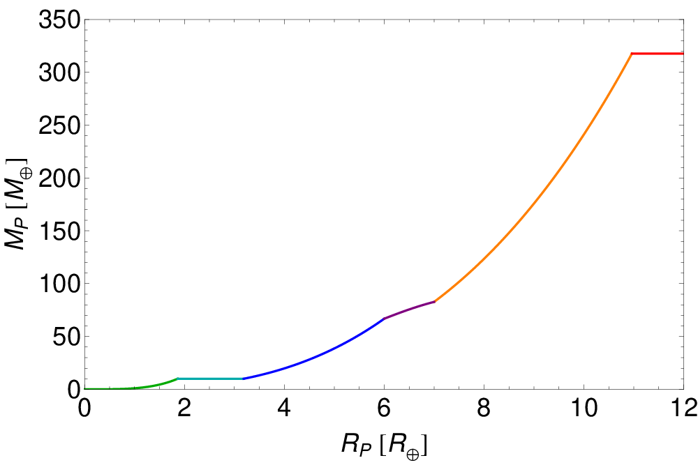
In this revised TSA algorithm, we make two major changes to the mass function: 1) we ensure a continuous mass-function 2) we allow this mass function to go into the Jupiter-regime. The first improvement is inspired by the fact that in the Super-Earth/Neptune regime, the Valencia et al. [50] mass function quickly exceeds 10 , which leads to an abundance of TSA targets at this boundary (since higher mass planets have a better chance of hosting a moon). The second improvement allows us to consider the Jupiters as well and thus expand our search somewhat.
The Valencia et al. [50] expression of is invertible to , in units of Earth radii and masses. For the mass hits 10 , which we consider a sensible upper limit for Super-Earth masses. Recall that TSA is primarily interested in a conservative estimate of the planetary mass in order to ensure selected candidates have the best chance of being a good target. We therefore consider the Super-Earth regime to be modified by this new radius limit. To bridge the gap between Super-Earths and Neptunes in a continuous manner, we fix the mass to be until , which occurs for (we assume spherical planets). The region between is dubbed “Mini-Neptunes” and such objects are assumed to have a mass of 10 .
Our previous boundary between Neptunes and Jupiters is also discontinuous. The mass of Jupiter-radius planets varies widely, but a sensible lower limit is to assume a Jovian bulk density. Much lower-density Jupiters do exist, so called inflated gas giants, but are thought to be due to their high irradiation environment since they are typically hot-Jupiters [8]. TSA automatically excludes hot-Jupiters since they are too close to their star to maintain an exomoon [52]. We therefore adopt a Jovian density of 1.326 g cm-3. To bridge the density discontinuity between Neptunes and Jupiters, we assume the bulk density linearly drops off between 6 and 7 to create a continuous mass function. Finally, for a Jovian density object, once the radius exceeds the mass will exceed a Jupiter mass11 1 This does not occur at km 1 since this the equatorial radius of Jupiter and the planet is non-spherical.. For such cases, we set the upper limit on the mass to be 1 . This is again in line with the conservative mass estimate requirements of TSA. In summary, we have:
- i)
“Super-Earths”;
- ii)
“Mini-Neptunes”;
- iii)
“Neptunes”;
- iv)
“sub-Jupiters”;
- v)
“Jupiters”;
- vi)
“super-Jupiters”;
These six regimes are described by the following mass-function:
where
| (1) |
II.1.3 TSA inputs
The TSA algorithm can be executed for several different inputs. Critically, one can choose the maximum orbital distance that an exomoon can reside at (in units of the Hill radius) , and the tidal dissipation factor of the host planet , both of which strongly affect the maximum allowed exomoon mass via the expressions of Barnes & O’Brien [4]. TSAs are defined to satisfy the criterion that the host planet can maintain an Earth-mass moon for 5 Gyr [34] and thus these inputs affect the number of TSA candidates identified.
An additional freedom is that one can alter the requirement of the signal-to-noise ratio (SNR) for a moon transit. We define SNR as an Earth-radius transit depth divided by the combined differential photometric precision (CDPP) [13] over 6 hours (see Equation 2). Note that the CDPP values are taken from the B12 tables, as with all other TSA inputs. One can see that enforcing a higher SNR condition will naturally reduce the number of TSA candidates found.
| (2) |
Finally, one can choose whether we look at host planets in the Neptune-regime and smaller or whether we expand our search to include Jupiter-sized objects (which tend to have a higher false-positive-rate, Santerne et al. 46). In this work, we treat quarters 1 to 9 from Kepler as the survey data used to look for exomoons. This leads to another criterion for TSA that days, so that at least three transits exist in the Q1-9 Kepler photometry; a minimum requirement for exomoon searches. At the time of writing, Q10-13 have also recently become available and we treat these data as follow-up photometry with application for particularly interesting candidates. Any candidate already selected as a target of opportunity (TSO) by the HEK project was not included in the TSA lists. We summarize the results of making these modifications in Table 1.
II.1.4 TSA results
| Candidates found | ||
| 0.9309 | ||
| 0.4805 | ||
| 0.3333 | ||
| 0.2500 | ||
| 0.9309 | ||
| 0.4805 | ||
| 0.3333 | ||
| 0.2500 | ||
| 0.9309 | ||
| 0.4805 | ||
| 0.3333 | ||
| 0.2500 | ||
| 0.9309 | ||
| 0.4805 | ||
| 0.3333 | ||
| 0.2500 |
Curiously, Table 1 reveals that Jupiter-sized objects offer very little improvement in the number of viable candidates for moon hunting. This is certainly due to a dearth of Jupiter-sized objects in the Kepler-sample more than anything else (B12).
For regular satellites, such as the Galilean satellites around Jupiter, the formation of large moons is enhanced by a massive primary [9, 47, 42]. However, if the proposed mass scaling law of [9] holds true, that , then such moons will be undetectable using Kepler [25]. The moons we seek are therefore most likely irregular satellites arriving through capture or impact (e.g. Triton-Neptune Agnor & Hamilton 1). In such a case, Porter & Grundy [44] argue that the mass of the primary has a much weaker effect with Neptunes and Jupiters retaining captured satelites with broadly equivalent efficiencies. It is therefore important to stress that Jupiter-sized KOIs do not hold a special significance for target selection over Neptunes.
Due to the relatively small improvement in the overall number of candidates offered by Jupiters, combined with their higher false-positive rate [46], we will not consider Jovian TSA candidates in this work, but we will return to them later in a future HEK survey.
II.1.5 Selecting a TSA category
Table 1 presents twenty-four different viable inputs for the TSA algorithm (for Neptunes or smaller). We must now select which input to use. The first point to bear in mind is that an excellent candidate will appear in multiple categories. For example, if a candidate satisfies SNR then it will of course also satisfy SNR. The task is therefore simply to move from the most conservative estimate to the most optimistic and stop at the point at which we have the desired number of candidates.
Due to computational constraints, we estimated we could analyze a handful of targets in this work. We therefore attempted to select a category which yields around a dozen or so candidates and apply the final target selection prioritization (TSP) stage to filter out the best of those.
We choose to work with in what follows, since this option finds dramatically more high SNR signals and thus the best chance for success. Next, we only consider candidates where the expected SNR to balance between a high SNR and a significant number of candidates. We only consider KOIs with radii below (as reported by B12) for reasons discussed earlier. Finally, we opt for which bounds all prograde satellites yet still returns 35 TSA candidates, which are listed in Table 2.
| KIC | KOI | [days] | SNR (B12) | (MAST) | Multiplicity |
| 3425851.01* | 268.01 | 110.4 | 5.76 | 1 | |
| 11623629.01 | 365.01 | 81.7 | 6.39 | 1 | |
| 7296438.01 | 364.01 | 173.9 | 4.68 | 1 | |
| 5966322.01 | 303.01 | 60.9 | 2.62 | 1 | |
| 8292840.02 | 260.02 | 100.3 | 2.69 | 2 | |
| 9451706.01 | 271.01 | 48.6 | 2.32 | 2 | |
| 9414417.01* | 974.01 | 53.5 | 2.28 | 1 | |
| 9002278.03 | 701.03 | 122.4 | 2.18 | 3 | |
| 9965439.01 | 722.01 | 46.4 | 2.22 | 1 | |
| 11622600.01 | 1876.01 | 82.5 | 3.17 | 1 | |
| 7199397.01* | 75.01 | 105.9 | 2.61 | 1 | |
| 11297236.01 | 1857.01 | 88.6 | 2.10 | 1 | |
| 9349482.01* | 2020.01 | 111.0 | 3.72 | 1 | |
| 10810838.01 | 174.01 | 56.4 | 2.04 | 1 | |
| 10471621.01 | 2554.01 | 39.8 | 3.19 | 2 | |
| 7761545.01 | 1472.01 | 85.4 | 2.60 | 1 | |
| 8686097.01 | 374.01 | 172.7 | 2.09 | 1 | |
| 12121570.01 | 2290.01 | 91.5 | 2.73 | 1 | |
| 9661979.01 | 2132.01 | 69.9 | 2.11 | 1 | |
| 2449431.01 | 2009.01 | 86.7 | 3.82 | 1 | |
| 2443393.01 | 2603.01 | 73.7 | 2.46 | 1 | |
| 5526717.01 | 1677.01 | 52.1 | 2.65 | 2 | |
| 10027247.01 | 2418.01 | 86.8 | 3.66 | 1 | |
| 11037335.01 | 1435.01 | 40.7 | 2.22 | 2 | |
| 12400538.01 | 1503.01 | 76.1 | 2.00 | 1 | |
| 10015937.01 | 1720.01 | 59.7 | 3.98 | 1 | |
| 11656918.01 | 1945.01 | 82.5 | 2.31 | 2 | |
| 11176127.03 | 1430.03 | 77.5 | 3.18 | 3 | |
| 8611781.01 | 2185.01 | 77.0 | 2.34 | 1 | |
| 8892157.02 | 2224.02 | 86.1 | 2.92 | 2 | |
| 6765135.01 | 2592.01 | 175.6 | 2.53 | 1 | |
| 8758204.01 | 2841.01 | 159.4 | 3.49 | 1 | |
| 9030537.01 | 1892.01 | 62.6 | 4.18 | 1 | |
| 8240904.02 | 1070.02 | 107.7 | 2.66 | 3 | |
| 8240904.03 | 1070.03 | 92.8 | 2.66 | 3 |
II.2. Target Selection Prioritization (TSP)
II.2.1 Overview
The TSA algorithm has identified 35 KOIs as being suitable for an exomoon analysis. With this more manageable number, we can apply some more time intensive selection criteria as part of the target selection prioritization (TSP) process. In this work, we consider three TSP criteria, which sequentially increase in time requirements to evaluate:
-
KOI must be in a single-transiting system
-
SNR should hold-up when queried from the MAST archive
-
KOI should not exhibit excessive time-correlated noise
We discuss each of these three criteria in the following subsections.
II.2.2 Multiplicity
The first criterion eliminates KOIs which would require a more complicated and involved analysis due to their multiple nature. Multiples should induce transit timing variations (TTVs) on one another, which is also a signature of exomoons. Eliminating these KOIs does not eliminate the possibility of planet-induced TTVs by any means (as recently demonstrated by the counter-example of KOI-872 Nesvorný et al. 41), but it does make our task simpler. Later HEK surveys may relax this constraint. Of the 35 TSAs, 11 were found to reside in multiple transiting systems and were rejected.
II.2.3 Cross-referencing CDPPs
The TSA algorithm works by reading in a list of planet and star parameters for each KOI. The major source for such parameters comes from B12. This work also includes estimates of the CDPP over 6 hours timescale, which TSA uses to estimate the SNR. During our investigation, we noticed several cases where the CDPP values reported in the tables of B12 did not agree with those reported by MAST when queried. We therefore decided to cross-reference the SNRs calculated from the B12 CDPP to those given by MAST.
In addition to the CDPP values differing between B12 and MAST, KOIs with a low host star may yield unreliable estimates for reasons discussed in detail in Muirhead et al. [40]. These authors provide improved estimates for such systems, which we use where available to compute a revised SNR. Since MAST provides the CDPP values for each quarter, we evaluate the mean and standard deviation of the SNR across all LC quarters.
We find that 12 of the remaining 24 KOIs have a mean SNR when we used the revised values and these candidates are summarily rejected. This leaves us with 12 KOIs.
II.2.4 Removing KOIs with excessive time-correlated noise
With 12 KOIs remaining, we are now ready to consider the most time-consuming TSP test. In the limit of a perfectly well-behaved star and instrument, the noise should be purely due to photon noise and thus behave as a Poisson distribution. Since the number of photons is large, the noise is very well described as a Gaussian distribution and has no frequency dependency; so-called “white noise”.
Time-correlated noise refers to noise which has the property that the probability distribution of values for a given measurement is not independent of previous measurements. This is a problem for the HEK project since time-correlated noise can mimic dips, bumps and distortions due to an exomoon. Whilst many methods exist to tackle time-correlated noise, they require various assumptions about the data’s behavior and invariably greater computational overhead. Since a significant fraction of Kepler’s targets have their photometry dominated by uncorrelated noise [22], the simplest strategy to deal with time-correlated noise is reject any KOIs exhibiting an excess on the timescale of interest. On timescales of days to weeks, one invariably finds time-correlated flux modulations, which could be considered a form of time-correlated noise, typically due to focus drift or stellar rotation. However, the timescale of interest for transiting exomoons is of order-of-magnitude one hour. Therefore, these long term variations do not affect our analysis and should be detrended out appropriately (see §III).
At this timescale of interest, it makes no difference to us whether excessive time-correlated noise is of instrumental or stellar origin since we have no intention of attempting to correct for it. Instead, our strategy is simply to reject all candidates showing excessive time-correlated noise. The question then becomes, what do we define as excessive time-correlated noise?
There is a dizzying number of metrics at our disposal for this task and we here seek a simple, computational efficient expression. A classic metric is the Durbin & Watson [17] statistic, , which uses autocorrelation to test whether a time series is positively or negatively autocorrelated. The Durbin-Watson statistic is given by
| (3) |
where are the residuals and is the number of data points. The value of always lies between 0 and 4, with 2 representing an absence of autocorrelation, representing positively-autocorrelated noise (expected for instrumental/astrophysical sources) and representing negatively-autocorrelated noise (anomalous and unphysical; we do not expect to see a significant excess of this).
In calculating , there exists a degree of freedom regarding over what cadence should we evaluate the statistic i.e. what timescale do we consider most relevant for an exomoon search? An exomoon transit or distortion could occur on a timescale of a few minutes or a few hours and so we selected 30 minutes for the simplicity that no binning is required for LC data and that the timescale is consistent with exomoon features. The next question is what value of should one consider acceptable?
Although test statistics are available via lookup tables for instance, these statistics assume regularly spaced time series which we often do not have for Kepler data, mostly due to outlier rejections and data gaps. Instead of using such statistics, we generate 1000 Monte Carlo simulations of Gaussian noise for the exact time sampling of a given data set to reproduce the expected posterior distribution of for data with no time-correlated noise. The Gaussian noise is generated assuming each data point is described by a Gaussian distribution with a standard deviation given by its associated uncertainty and a mean of unity.
The quantity is only calculated on data locally surrounding transits to within twice the timescale of the Hill sphere, (with the planetary transit itself excluded), since only this data is relevant for our exomoon hunt. We compute for each and every transit event and then take the mean over all transit epochs, . The same process is applied to the 1000 synthetic time series, which behave as Gaussian noise with the exact same cadence and time sampling as the original data. We also apply the same final-stage local linear detrending used on the real data to every synthetic data set (as is described later in §III). The 1000 synthetic time series are converted into 1000 metrics in the same as the original data and this is used to compute a probability distribution of in the case of Gaussian noise.
We then compare the real metric with the simulated distribution to evaluate whether our data set is consistent with a lack of autocorrelated noise. Any KOIs which show autocorrelation (as determined by the metric) in both the PA (Photometric Analysis) and PDC (Pre-search Data Conditioning) detrended LC data are rejected (SC data is not used in this selection phase but is used later). We do not anticipate that this will remove genuine moon signals since such events would be temporally localized rather whereas autocorrelation at a 30 minute timescale must be present throughout the entire time series (for the particular transit epoch under analysis). After applying this test to each target, we find that only 7 of the 12 remaining KOIs pass this test, as listed in Table 3. Note that all 12 KOIs were fully detrended in exactly the same way, as is described in §III. However, only 7 of these 12 are actually fitted with a transit light curve model - the most resource intensive stage of the entire process.
| KOI | of LC | (1-FAP) of autocorrelation () |
|---|---|---|
| KOI-364.01 | - | - |
| KOI-303.01 | ||
| KOI-974.01 | ||
| KOI-268.01 | ||
| KOI-1472.01 | ||
| KOI-722.01 | ||
| KOI-365.01 | ||
| KOI-174.01 | ||
| KOI-75.01 | ||
| KOI-2020.01 | ||
| KOI-1857.01 | ||
| KOI-1876.01 |
III. DETRENDING THE DATA WITH CoFiAM
Data is detrended using a custom algorithm which we dub Cosine Filtering with Autocorrelation Minimization (CoFiAM), which is described in this section.
III.1. Pre-Detrending Cleaning
In all cases, we performed the detrending procedure twice; once for the PA data and once for the PDC-MAP data. In what follows, each transit is always analyzed independently of the others i.e. we obtain a detrended light curve unique to each transit event, not each quarter. The first step is to visually inspect each quarter and remove any exponential ramps, flare-like behaviours and instrumental discontinuities in the data. We make no attempt to correct these artefacts and simply exclude them from the photometry manually. We then remove all transits using the B12 ephemerides and clean the data of 3 outliers from a moving median smoothing curve with a 20-point window (for both LC and SC data).
III.2. Cosine Filtering with Linear Minimization (CoFiAM)
The remaining unevenly spaced data is then regressed using a discrete series of harmonic cosine functions, which act as a high-pass, low-cut filter [2]. The functional form is given by
| (4) |
where is the total baseline of the data under analysis, are the time stamps of the data, & are model variables and is the highest harmonic order. Equation 4 may be more compactly expressed as a cosine function with a phase term, but the above format illustrates how the equation is linear with respect to and . This means that we can employ weighted linear minimization, which is not only computationally quicker than non-linear methods, but also guaranteed to reach the global minimum. In our regression, the data are weighted by the inverse of their reported standard photometric errors.
Harmonic filtering has been previously used to correct CoRoT (e.g. Mazeh et al. 39) and Kepler light curves (e.g. Kipping & Bakos 30; Kipping & Bakos 31; Kipping & Spiegel 32) and is attractive for its simplicity, computational efficiency and ability to preserve the transit shape.
III.3. Frequency Protection
There are many possible choices of , but above a certain threshold the harmonics will start to appear at the same timescale as the transit shape and thus distort the profile, which is undesirable. The transit light curve of a planet can be considered to be a trapezoid to an excellent approximation, for which an analytic Fourier decomposition is available. Waldmann [51] showed that a equatorial trapezoidal transit light curve is described by the following Fourier series:
| (5) |
Under the approximation of a trapezoidal light curve then, the lowest frequency is thus . Another way of putting this is that the highest periodicity is (i.e. the transit duration) and so if we protect this timescale, and all shorter timescales, the transit light curve should be minimally distorted. Let us therefore choose to protect a timescale , where is a real number greater than unity and is the first-to-fourth contact duration reported in B12. The timescale can be protected by imposing
| (6) |
Ideally, one would wish to impose in all cases to provide some cushion, but in reality such a condition means is small and the ability of the regression algorithm to obtain a reasonable fit to the data becomes poor. In contrast, going to higher values of leads to a better regression in the sense, but increases the risk of higher harmonics distorting the transit profile since strictly speaking we require . Therefore, there exists a trade-off between these two effects and one might expect an optimal choice of to exist for any given data set. Selecting such an optimum requires a quantitative metric which we aim to optimize.
III.4. Autocorrelation Minimization
For any optimization problem, one must first define what it is we wish to optimize or minimize. In this work, we identify the primary objective to be that the transit light curve contains the lowest possible degree of time-correlated noise around each transit, which could lead to false-positive moon signals. We therefore require some metric to quantify the amount of autocorrelation and optimize against. As discussed earlier, the Durbin-Watson statistic is a useful tool to this end and evaluates the degree of first-order autocorrelation in a time series. Our objective is therefore to choose a value of such that the Durbin-Watson statistic is consistent with the lowest quantity of autocorrelation, when evaluated on the data surrounding the planetary transit. Another way of putting this is that we wish to choose the value of which minimizes , when evaluated on the data within of the time of transit minimum (where is the Hill timescale).
Before we can begin our optimization search, one must define the allowed range of through which we can search. Recall that our expressions protect a timescale and thus one must choose in order to not disturb the transit profile. Consequently, we chose the lowest allowed value of to be 3, such the timescale is never perturbed. This factor of three cushion is to allow for transit duration changes, leakage of the harmonics for real transits and longer exomoon transits. Protecting this timescale corresponds to a maximum allowed value of of
| (7) |
Our detrending algorithm, CoFiAM, regresses the Kepler time series to the harmonic series given by Equation 4 in a least squares sense and repeats this regression for every possible integer choice of between 1 and . In this way, we explore dozens of different regressions which all satisfy the conditions of providing a good least squares fit to the light curve and protect a timescale . We then simply scan through the final list of values and define the optimal detending function to be the harmonic order which minimized when evaluated on the out-of-transit data within of the eclipse. If a quarter contains more than one transit, we always repeat the entire procedure for each transit to ensure the data associated with the transit is fully optimized for our exomoon hunt.
As before, the statistic is computed on a timescale of 30 minutes which means that no binning is required for the LC data. For the SC data, we bin the data up the long-cadence data rate.
Once the optimal detrending function has been found, we divide all data within (including the transit) by to correct for the long-term variations. We also apply a second outlier rejection of 10 filtering (to allow for unusual anomalies in the transit) from a moving 5-point median. For short-cadence data, we instead use a 3 filtering on a 20-point moving median. In some cases, we relaxed this outlier rejection when we felt the filter was removing potential exomoon signals. We clip out the data within and apply a linear fit through the out-of-transit data to remove any residual trend, which acts as a final normalization. The process is repeated for all transits and the surviving light curves are stitched together to form a single input file for our fitting code. Any transit epoch with data points in the window is accepted into the final file. Additionally, the final file always uses SC data over LC data, where such data exists.
IV. LIGHT CURVE FITS
IV.1. Overview
Model light curves of a transiting planet are generated using the LUNA algorithm described in Kipping [28]. LUNA is an analytic photodynamic light curve modeling algorithm, optimized for a planet with a satellite. LUNA accounts for auxiliary transits, mutual events, non-linear limb darkening and the dynamical motion of the planet and its satellite with respect to the host star. In the case of a zero-radius and zero-mass satellite, the LUNA expressions are equivalent to the familiar Mandel & Agol [38] algorithm.
For any given model, we regress the data to the model parameters using the MultiNest algorithm [18, 19]. MultiNest is a multimodal nested sampling (see Skilling 49) algorithm designed to calculate the Bayesian evidence of each model regressed, along with the parameter posteriors. By comparing the Bayesian evidences of different models, one may conduct Bayesian model selection, which has the advantage of featuring a built-in Occam’s razor. For each KOI in our survey, we always regress the following models as a minimum requirement:
-
Planet-only model with variable baselines using theoretical quadratic limb darkening coefficients; model .
-
Planet-only model with variable baselines and free quadratic limb darkening coefficients; model .
-
If , then we repeat fixing the LD coefficients to the maximum a-posteriori LD coefficients from model (the best LD coefficients will be adopted throughout from this point on), in a fit which we dub as .
-
Planet-only model with flat baseline over all epochs, . If then we use a flat baseline in all following fits (to reduce the number of free parameters), which was found to be always true thanks to CoFiAM employing a final-stage normalization.
-
Planet-only model with variables times of transit minimum (i.e. TTVs); model .
-
Planet-only model with each transit possessing unique transit parameters to allow for both TTVs and TDVs; model .
-
Planet-with-satellite fit; model .
-
Planet-with-satellite fit assuming a zero-mass moon; model .
-
Planet-with-satellite fit assuming a zero-radius moon; model .
The question as to why we switch from local baselines to a global baseline is discussed in the next subsection, §IV.2. In all fits, we use the same data set throughout, which is usually the PA data. This is because the PDC-MAP data is subject to numerous detrending processes that do not necessarily preserve exomoon signals. However, if the PA data yields a statistic with more than 3 confidence of autocorrelation but the PDC-MAP is below 3 , then the PDC-MAP data is used in the fits instead. However, Table 3 reveals how there is no such instance in the sample of KOIs studied in this work.
IV.2. Planet-only Fits
The first stage of our fitting process always begins with planet-only fits. The purpose of these fits is to i) verify or obtain reliable limb darkening parameters ii) serve as a baseline for comparison with the planet-with-moon fits. Initially, we employ fixed limb darkening coefficients, calculating theoretical values from a Kurucz [36] style-atmosphere integrated over the Kepler-bandpass. The computation is performed by a code written by I. Ribas and associated details can be found in Kipping & Bakos [30].
In these fits, the five basic transit parameters are , , , and . The choice of these five parameters is fairly commonplace in the exoplanet literature, except for perhaps . This parameter is used so that the posteriors of have a uniform prior and can be utilized with the Multibody Asterodensity Profiling (MAP) technique, as discussed in Kipping et al. [33]. Although it is not the purpose of this work to conduct MAP, the posteriors are available upon request so that these studies can be facilitated in the future without re-executing the light curve fits.
For all KOIs, an estimate of and exists from B12 which we use to define a uniform prior of day either side of the estimate for both and . The other three basic parameters also have uniform priors of , and kg2/3 m-2 kg2/3 m-2 (covering the main-sequence of stars between spectral types of M5 to F0 with a factor of 10 cushion at each boundary Cox 15). The transit epoch, , can be centered on any one of the transits in the Q1-9 time series. We choose an epoch which is nearest to the median time stamp of Q1-9 data, in order to minimize degeneracy between and in the fits [43].
Whether the fit is using a variable baseline () or a flat baseline (), we adopt a uniform prior of . For model, the total number of free parameters to be marginalized over (and thus explored by MultiNest) is just 5+1=6. The model has 5+ free parameters. Experience with MultiNest shows that fitting models with more than 20 free parameters becomes dramatically more time-consuming and so the flat baseline model is useful later for exomoon fits with a greater number of basic parameters. It is for this reason that we transition from local baselines to a global baseline as the model complexity increases.
When fitting for limb darkening parameters, we use quadratic limb darkening so that only two degrees of freedom are required, yet the curvature of the light curve can be modelled effectively [14]. For consistency, we employ quadratic limb darkening when we use the fixed limb darkening parameters too. We fit for the terms and since they are bounded by the physically motivated lower and upper limits of and (see Carter et al. 11 and Kipping et al. 34).
In both the planet-only fits, and all subsequent fits, we account for the integration time of the long-cadence data using the resampling method [26] with (as generally recommended in Kipping 26). All MultiNest fits will also employ 4000 live points, as recommended by Feroz et al. [19] for evidence calculations.
IV.3. TTV & TDV Fits
A transit timing variation (TTV) fit is performed by assigning each transit epoch a unique time of transit minimum, . All other parameters are kept global as before in . This TTV fit is dubbed . The period prior is changed to a Gaussian prior assigned from the posterior of from the model fits. Without a constraining prior on , allowing every transit epoch to have a unique transit time would mean that would be fully degenerate with the parameters.
Transit duration variations (TDVs) may be due to velocity changes or impact-parameter changes of the observed planet. These changes induce not only changes in the transit duration, but changes in the derived (and thus ) and . We also search for changes in the apparent value due to spot activity or exomoon mutual events, for example. Additionally, TDVs are expected to occur in dynamic systems exhibiting TTVs too. With so many degrees of freedom required, the fits would certainly involve a large number of free parameters making the regression very time consuming with MultiNest. To solve this, one may paradoxically increase the number of degrees of freedom again by allowing for variable baselines (OOT). By doing so, all six transit parameters are independent for each epoch (i.e. there are no fitted global parameters) and thus the fits can be conducted on each epoch separately and then the sum of the log Bayesian evidences will give the global log Bayesian evidence. These individual transit fits are very fast to execute and may be run simultaneously. For these reasons, we dub the regression meaning variable transit parameters for each epoch and the subscript V denotes variable baselines too.
TDVs may be defined in several ways, unlike TTVs which have less ambiguous definition. In this paper, we define the TDVs to be the variation of the parameter , where is the duration for the planet’s center to enter to stellar disc and subsequently leave. We use this definition rather than the first-to-fourth contact duration, for example, since has the lowest relative uncertainty when the limb darkening coefficients are fixed [10]. We divide this duration by two since the theoretical uncertainties on are exactly twice that of [10] and thus our derived TTVs and TDVs should exhibit similar scatter and scale, which makes for useful comparisons.
IV.4. Planet-with-Moon Fits
In general, we make the following assumption: exomoons may be randomly oriented but have nearly circular orbits due to tidal dissipation (e.g. see Porter & Grundy 44, Heller & Barnes 20). Therefore, our survey-mode fits do not consider fitting for the orbital eccentricity of the exomoon. We find that this dramatically improves the speed and stability of our fits using MultiNest.
In contrast to exomoons, there is no reason to expect exoplanets to have zero eccentricity, especially at long periods, due to the much longer circularization timescales and the possibility for planet-planet forcing or Kozai migration. Despite this, we choose to assume a circular orbit in the survey light curve fits in this paper. The advantage of doing so is firstly to save MultiNest exploring an additional two free parameters and secondly to save solving Kepler’s equation numerically at every time stamp.
We justify our choice on the basis that the maximum stable orbital separation of a moon decreases rapidly with respect to the host planet’s orbital eccentricity, as shown by Domingos et al. [16]. Here, the authors find the maximum separation scales as . Further, the maximum stable exomoon mass around a host planet scales as this separation to the index of , as shown by Barnes & O’Brien [4]. We therefore expect that the maximum moon mass around a host planet scales as . On this basis, an eccentricity of even 0.1 halves the maximum stable exomoon mass and an eccentricity of 0.3 reduces it by an order-of-magnitude. Future HEK surveys may explore eccentric planet solutions, but for this paper computational constraints limit our survey to circular systems for the reasons discussed.
Another assumption we make is that exomoons orbit in a prograde sense. The gravitational influence of a satellite induces transit timing variations (TTV) and velocity-induced transit duration variations (TDV-V) [23]. Both of these effects are insensitive to the sense of the moon’s orbital motion. Additionally, satellites induce transit impact parameter induced transit duration variations (TDV-TIP), which typically have an amplitude of around an order-of-magnitude less than that of TDV-V. However, TDV-TIP is sensitive to the sense of orbital motion [24]. Therefore, by treating all exomoons as prograde in our survey, a retrograde moon would have not its TDV-TIP effect modeled correctly and thus an implicit assumption is therefore that TDV-VTDV-TIP. As with the eccentricity assumption, this allows us to halve the parameter volume to be scanned through and thus expedite the fitting procedure.
In addition to the standard planet-with-moon model, we try two “unphysical” fits where we fix the moon’s mass and then the radius to be zero. These fits are useful in the vetting stage since a moon detection should not yield an improved Bayesian evidence with unphysical properties, such as zero-radius. These fits are dubbed and for the zero-mass and radius cases respectively.
A careful choice of the parameter set and priors is crucial for the moon’s parameters, since the expected signal-to-noise is low and thus priors can be expected to play an increasingly significant role in the derived results. In Kipping et al. [34], we suggested , , , , , and with uniform priors for all. In this work, we have found that these priors were not fully adequate and our greater experience has led us to propose a modification. Firstly, is now fitted with a Jeffrey’s prior since it spans several orders of magnitude and the low periods require dense sampling due to the bunching up of harmonics. Secondly, we have exchanged for to impose an isotropic prior. Thirdly, we have exchanged for (the separation between the planet and moon in units of the planetary radius). This last change is geometrically motivated and means that MultiNest scans for moon transits evenly in time and space from the primary planet event. Except for , all terms have uniform priors.
The parameter has the intuitively obvious prior of . Similarly, we use for and with the exception that the boundary conditions are periodic and thus the parameters are considered “wrap-around” parameters in MultiNest. The mass and radius ratios have the very simple boundary conditions of being between zero and unity i.e. .
The upper boundary condition on is given by , which represents the edge of the Hill sphere as proved by Kipping [23] (i.e. ). The lower boundary is less obvious and in Kipping et al. [34] we proposed hours as a rough estimate. Since , the maximum size of the moon is . If this is the case, then the closest separation allowed before contact would occur is . On this assumption, one may derive a lower limit for . From Equation 7 of Kipping [27], one can re-arrange to make the subject:
| (8) |
Substituting with and then replacing with the minimum allowed value of we have:
| (9) |
Exploiting the fact and cleaning up the expression we find:
| (10) |
The maximum allowed value of is 2 and the maximum physically plausible value of is 27950 kg m-3 [34]. This yields days (1.25 hours) which we employ as our lower boundary condition for .
For , the lower boundary condition is simply 2, which for guarantees no contact (for a circular satellite orbit). The maximum requires another small derivation. We consider the maximum to be the Hill sphere, ; therefore we have:
| (11) |
Replacing the mass terms with densities, we obtain:
| (12) |
If we assume , then which can be substituted into the above expression to give:
| (13) |
To estimate this value, we adopt the maximum allowed planetary density of kg m-3 [34] and use the maximum a-posteriori value of from the planet-only fits (technically model ). is then fitted with a uniform prior between 2 and this maximum value.
Finally, we instruct MultiNest to ignore any trials which yield an unphysical density for the planet, which we consider to be between kg m-3 and kg m-3 [34]. We apply the same constraint to the satellite except the lower allowed limit is 0 kg m-3. This is imposed so that zero-mass moons can be explored meaning that in the case of a null-detection the posterior of can still reach zero. For models, and we deactivate the constraint on the satellite density since the satellite is specifically defined to be unphysical.
IV.5. Detection Criteria
An exomoon has never been detected and thus one is forced to seriously consider what constitutes a “detection” in such a new area. The signal-to-noise will inevitably be at, or close to, the limit of Kepler, the signal will vary in phase and time and may manifest simply as a slight distortion to a planet’s transit profile. If one fits a planet-with-moon model to real data, the extra degrees of freedom will inevitably lead to an improved relative to a planet-only fit. Clearly an improved is not sufficient to claim an exomoon has been found. This concern was one of the driving reasons why the HEK project adopted Bayesian model selection [34] available through MultiNest, since such comparisons implicitly penalize models for using extra parameters (Occam’s razor). However, even the Bayesian evidence is not a tool which can be wielded blindly to claim exomoon detections.
Although our detrending process CoFiAM minimizes the amount of autocorrelation, the data will always possess some quantity of time-correlated noise. The likelihood function employed by LUNA is a Gaussian likelihood expression (see Equation 20 of Kipping et al. 34) and so this assumption will never be strictly true. It is therefore possible, and in fact quite common, that the Bayesian evidence of a planet-with-moon fit will be superior to a planet-only fit for an isolated planet, even with the built-in Occam’s razor of Bayesian model selection. A possible remedy would be to employ a more sophisticated likelihood function but the computational demands of MultiNest make this unrealistic as fits typically take weeks to run even on modern clusters. Instead, we stress that a superior Bayesian evidence is not tantamount to a detection with exomoon fits since LUNA can generate distortions both in- and out-of-transit which can describe certain time-correlated noise features.
We therefore consider that a superior Bayesian evidence of a planet-with-moon fit to a planet-only fit (i.e. ) is a requirement for a “detection”, but not a proof in of itself. As discussed in Kipping et al. [34], we set the significance level of this improvement to be in 4 or greater in order to qualify. This discussion therefore indicates that other detection criteria are required.
One of the easiest tests is that the posteriors should be physically plausible. For example, as shown in Kipping [27], exomoons allow us to measure the ratio and which for an assumed yields . It is easy to check whether the derived is consistent with the derived from known planet populations. For example, a candidate planet yielding a Jupiter-mass and an Earth-radius can be easily dismissed.
Further, a planet-with-moon model must be superior to both unphysical moon models considered i.e. the zero-mass moon and the zero-radius moon models. If the zero-mass moon model is superior, one should suspect starspots or correlated noise to be responsible. If the zero-radius moon is superior, one should suspect TTVs from a non-moon origin. In both cases, it is also possible that the signal-to-noise of the moon signal is presently too low to make a confirmed detection (but more data may change this).
We also require that both the mass and radius of the exomoon can be considered independently detected. This means that the posteriors of both and must not be converged at zero in the planet-with-moon fits. These battery of tests form our requirements for an exomoon to be considered plausible and so far we have described four basic detection criteria, summarized as:
- B1
Improved evidence of planet-with-moon fits at confidence
- B2
Planet-with-moon evidences indicate both a mass and radius preference
- B3
Parameter posteriors are physical (e.g. , )
- B4
Mass and radius of moon converge away from zero
Should these tests be passed or perhaps a candidate only marginally fails some of these criteria, we may consider further investigation. We discuss here three quick general follow-up criteria which can be implemented. Since this paper’s survey only uses Q1-9 data, subsequent Kepler data may be treated as follow-up photometry. One simple check then is that all four basic criteria are satisfied when the new data is included and the model refitted. Further, the significance of the moon candidate should be enhanced by the new data and yield broadly the same set of parameters. Without even fitting the new data, another simple check is to extrapolate the best-fit light curve model from the moon hypothesis into the times of the new observations and compare (in a sense) the “predictive power” of the moon model relative to a simple planet-only model. We summarize these general follow-up detection criteria below:
- F1
All four basic criteria are still satisfied when new data is included
- F2
The predicitive power of the moon model is superior (or at least equivalent) to that of a planet-only model
- F3
A consistent and statistically enhanced signal is recovered with the inclusion of more data
Even after passing all of these tests, the candidate should not be blindly accepted as a confirmed detection. Candidate specific tests and follow-up may be needed too, if for example the star shows rotational modulations and the candidate moon exhibits mutual events (which may in fact be star spot crossings). Exploration of perturbing planet solutions causing TTVs/TDVs may be needed, as in the case of Nesvorný et al. [41]. Target specific tests will be investigated appropriately should the need arise.
IV.6. Excluded Moons
In cases of null-detections, one of the aims of the HEK project is to provide limits on what moons can be excluded. There are many possible choices for which parameters we provide excluded limits. Two terms of particular interest are the mass ratio and the radius ratio (). In general, we find the radius ratio to be untrustworthy due to the effects of starspots and time-correlated noise. Further, the parameter is positively-biased since we impose a likelihood penalty for high-density (i.e. low-radius) moon solutions. Therefore, we opt to provide upper limits on the mass ratio for each null-detection.
The excluded limits must be understood in terms of the adopted priors. For example, when we posit that there is a 95% probability of there existing no moon of , the statement is only meaningful when combined with the adopted priors e.g. uniform prior in and Jeffrey’s prior in . This subtle point is important when interpreting the 95% and 3 quoted limits. However, we also make available the full posteriors revealing all relevant cross-correlations for those wishing to investigate the frequency of moons in more detail.
One caveat with the provided upper limits is that MultiNest may have located a spurious signal and spurious detections cannot be used to define upper limits on . Spurious detections occur because the code attempts to locate the best modes which explain the data i.e. the best model fits. In many cases, the solution can be dismissed using some of the detection criteria already discussed but the derived posteriors of and/or still converge to non-zero values due to perhaps time-correlated noise or starspots. Simply taking the 95% quantile of these posteriors does not technically translate to an excluded upper limit estimate. Indeed these upper limits can approach unity if the model fit converged to a binary-planet solution, for example. In such spurious detection cases, all we can say for certain is that we are unable to detect an exomoon but we caution that meaningful upper limits on and is not guaranteed for each system analyzed.
In addition to providing limits on , we also compute limits for two more observable-centric defined terms, the moon-induced TTV and TDV amplitudes. Specifically, we calculate the quantiles of the distribution of the root-mean-square (r.m.s.) amplitudes of the two effects using the expressions from Kipping [29], and . The TDV r.m.s. amplitude is defined as the sum of the TDV-V and TDV-TIP effects, for reasons discussed in Chapter 6 of Kipping [29]. It should be stressed that excluding a certain moon-induced TTV amplitude does not equate to excluding a TTV amplitude induced by other effects too (and similarly for TDV).
V. RESULTS
V.1. KOI-722.01
V.1.1 Data selection
After detrending with CoFiAM, the PA and PDC-MAP data were found to have a 1.7 and 1.9 confidence of autocorrelation on a 30 minute timescale respectively and therefore both were acceptable ( ). In general, we always prefer to use the raw data and so we opted for the PA data in all subsequent analysis of this system. Short-cadence data is available for quarter 9 and this data displaced the corresponding long-cadence quarter in our analysis.
V.1.2 Planet-only fits
When queried from MAST, the KIC effective temperature and surface gravity were reported as K and [6]. Using these values, we estimated quadratic limb darkening coefficients and (as described in §IV.2). The initial two models we regressed were and where the former uses the aforementioned limb darkening coefficients as fixed values and the latter allows the two coefficients to be free parameters. We find that indicating essentially no preference between the two models. Given that the data is equally well-described by either theoretical or fitted coefficients, we opt for the theoretical limb darkening coefficients since they are more physically motivated.
KOI-722.01 has a period of days (as determined by model ) and exhibits 14 complete transits in Q1-Q9 from epochs -8 to +8 (epochs +3, +4 and +7 are missing). As is typical for all cases, indicating that allowing for 14 independent baseline parameters is unnecessary relative to a single baseline term (thanks to the CoFiAM final stage normalizations).
We find no evidence for TTVs in KOI-722.01, with , which is formally an 7.2 preference for a static model over a TTV model. The timing precision on the 14 transits ranged from 5-17 minutes (see Table 4). The TTVs, shown in Fig. 2(a), show no clear pattern and exhibit a standard deviation of minutes and for 14-2 degrees of freedom.
The TTV+TDV model fit, , finds consistent transit times with those derived by model . We also find no clear pattern or excessive scatter in the TDVs, visible in Fig. 2(a). The standard deviation of the TDVs is found to be minutes and we determine for 14-1 degrees of freedom.


| Epoch | [BJDUTC] () | TTV [mins] () | [BJDUTC] () | TTV [mins] () | [mins] () | TDV [mins] () |
|---|---|---|---|---|---|---|
| -8 | ||||||
| -7 | ||||||
| -6 | ||||||
| -5 | ||||||
| -4 | ||||||
| -3 | ||||||
| -2 | ||||||
| -1 | ||||||
| +0 | ||||||
| +1 | ||||||
| +2 | ||||||
| +5 | ||||||
| +6 | ||||||
| +8 |
V.1.3 Moon fits
A planet-with-moon fit, , is preferable to a planet-only fit at a formally high significance level (7.5 ), passing detection criteriopn B1 (see Table 5). KOI-722.01 fails detection criterion B2 though, since a zero-mass moon model fit yields a higher Bayesian evidence at 2.8 confidence.
Investigating further, one finds the parameter posteriors to be ostensibly unphysical. Physical parameters of the candidate solution may be estimated by combining our posteriors with the estimated stellar parameters of B12 ( and ). The moon is found to lie at a highly inclined orbit and exhibit physically consistent parameters of and . In contrast, the planet has a very high density with parameters and . We consider these parameters to be likely unphysical and thus KOI-722.01 fails detection criterion B3. Finally, the posterior for does not converge away from zero and thus no mass signal can be considered to be detected, failing criterion B4. This is also consistent with the fact that a zero-mass moon model gave a higher Bayesian evidence. We therefore conclude the model fit of is an exomoon false-positive and no convincing evidence for a satellite around KOI-722.01 exists in Q1-9.
The origin of the false-positive is unclear as the maximum a-posteriori fit from reveals auxiliary transits (see Fig. 3), which cannot be caused by starspot crossings. In this case, we consider time-correlated noise to be the most likely explanation. The posterior converges on zero and we find the 95% quantile to be to the 3 quantile is (see Fig. 4(a)). Our final system parameters are provided in Table 6.

| Model, | ||
| Planet only fits… | ||
| - | ||
| Planet with timing variations fits… | ||
| Planet with moon fits… | ||


| Parameter | Value |
|---|---|
| Derived parameters… | |
| [days] | |
| [BJDUTC] | |
| [deg] | |
| [g cm-3] | |
| [hours] | |
| Physical parameters… | |
| [] | |
| [] | |
| [] | |
| [95% confidence] | |
| [mins] | (95% confidence) |
| [mins] | (95% confidence) |
V.1.4 Summary
We find no compelling evidence for an exomoon around KOI-722.01 and estimate that to 95% confidence. This assessment is based on the fact the system fails the basic detection criteria B2, B3 and B4 (see §IV.5).
V.2. KOI-365.01
V.2.1 Data selection
After detrending with CoFiAM, the PA and PDC-MAP data were found to have a 2.2 and 3.1 confidence of autocorrelation on a 30 minute timescale respectively. Since only the PA data is considered acceptable ( ), it will be utilized throughout the analysis that follows. Short-cadence data is available for quarters 3, 7, 8 and 9 and this data displaced the corresponding long-cadence quarters in our analysis.
V.2.2 Planet-only fits
When queried from MAST, the KIC effective temperature and surface gravity were reported as K and [6]. Using these values, we estimated quadratic limb darkening coefficients and . The initial two models we regressed were and , where the former uses the theoretical limb darkening coefficients as fixed values and the latter allows the two coefficients to be free parameters. We find that indicating that our limb darkening coefficients may not be optimal. The maximum a-posteriori limb darkening coefficients from the model fit were and , which we chose to treat as fixed terms in all subsequent model fits.
KOI-365.01 has a period of days (as determined by model ) and exhibits 9 transits from Q1-Q9. As is typical for all cases, indicating that allowing for 9 independent baseline parameters is unnecessary relative to a single baseline term.
We find no evidence for TTVs in KOI-365.01, with , which is formally an 8.3 preference for a static model over a TTV model. The timing precision on the 9 transits ranged from 1.3 to 2.8 minutes and yields a flat TTV profile, as shown in Fig. 2(b). We calculate a standard deviation of minutes and for 9-2 degrees of freedom.
The TTV+TDV model fit, , finds consistent transit times with those derived by model . No clear pattern or excessive scatter is visible in the data, shown in Fig. 2(b). We therefore conclude there is no evidence for TTVs or TDVs for KOI-365.01. The standard deviation of the TDVs is found to be minutes and we determine for 9-1 degrees of freedom.
| Epoch | [BJDUTC] () | TTV [mins] () | [BJDUTC] () | TTV [mins] () | [mins] () | TDV [mins] () |
|---|---|---|---|---|---|---|
| -5 | ||||||
| -4 | ||||||
| -3 | ||||||
| -2 | ||||||
| -1 | ||||||
| +1 | ||||||
| +2 | ||||||
| +3 | ||||||
| +4 |
V.2.3 Moon fits
A planet-with-moon fit, , is disfavored relative to a planet-only fit at (see Table 8) and so detection criterion B1 is not satisfied. The system also fails detection criterion B2 since a zero-mass moon yields an improved Bayesian evidence relative to a moon with finite mass.
We may combine the posteriors from with the stellar parameters derived by B12 ( and ) to obtain physical parameters for the planet-moon candidate system. We find that the planet has an unusually low density with and . The moon also has a low density with parameters and . Whilst these parameters are somewhat extreme they are not implausible, but at best detection criterion B3 can be considered unclear. Finally, the posterior fails to converge away from zero, failing detection criterion B4, and consistent with the fact that model is favored over model . We therefore conclude the model fits of and represent an exomoon false-positive and no convincing evidence for a satellite around KOI-365.01 exists in Q1-9.
The maximum a-posteriori model fit of (shown in Fig 5) does not exhibit any clear auxiliary or mutual events, despite converging away from zero. The reason for this becomes clear when one notes that the semi-major axis of the moon’s orbit around the planet converges to , which shows that the moon is in very close proximity to the planet. In such a case, the planet and moon appear almost on-top of one another and thus virtually no light curve distortion is visible. This one way in which a fitting algorithm can essentially “hide a moon” in the fits and such fits are always suspicious. The close proximity of the moon leads to an absence of TTVs too since TTVs scale as [23] and so the solution also masks the exomoon mass.
Unlike TTVs, TDVs scale as and so one might expect that the exomoon mass could not be hidden from TDVs too. However, the period of the moon solution is also short at d and this causes a problem for TDV inference. As noted in Kipping [29], traditional TDV theory breaks down if the moon accelerates/decelerates significantly during a transit duration and thus the theory only holds for . In this case, days and days meaning that that TDVs will not necessarily be present for even massive exomoons. Due to these points, close-binary moon solutions tend to yield less useful constraints on excluded mass and radius ratios. In this case, the moon fit yields a worse Bayesian evidence than a planet-fit and thus we know it is not the favored model, yet the upper limits are not as reliable as with KOI-722.01 for example. The posterior converges on zero and we find the 95% quantile to be and the 3 quantile is (see Fig. 4(b)). Our final system parameters are provided in Table 9.

| Model, | ||
| Planet only fits… | ||
| - | ||
| Planet with timing variations fits… | ||
| Planet with moon fits… | ||
| Parameter | Value |
|---|---|
| Derived parameters… | |
| [days] | |
| [BJDUTC] | |
| [deg] | |
| [g cm-3] | |
| [hours] | |
| Physical parameters… | |
| [] | |
| [] | |
| [] | |
| [95% confidence] | |
| [mins] | (95% confidence) |
| [mins] | (95% confidence) |
V.2.4 Summary
We find no compelling evidence for an exomoon around KOI-365.01 and estimate that to 95% confidence. This assessment is based on the fact the system fails the basic detection criteria B1, B2 and B4 and B3 is considered marginal (see §IV.5).
V.3. KOI-174.01
V.3.1 Data selection
After detrending with CoFiAM, the PA and PDC-MAP data were found to have a 1.5 and 0.6 confidence of autocorrelation on a 30 minute timescale respectively and therefore both were acceptable ( ). Since the PA data detrending shows no strong evidence of autocorrelation, we opted to use this less-manipulated data in what follows. Short-cadence data is available for quarters 3, 4, 5 and 6 and this data displaced the corresponding long-cadence quarters in our analysis.
V.3.2 Planet-only fits
When queried from MAST, the KIC effective temperature and surface gravity were reported as K and [6]. Using these values, we estimated quadratic limb darkening coefficients and . The initial two models we regressed were and , where the former uses the theoretical limb darkening coefficients as fixed values and the latter allows the two coefficients to be free parameters. We find that suggesting that our limb darkening coefficients could be improved. Strangely though, when we fix the limb darkening coefficients to the maximum a-posteriori values from the model fit, we actually obtain a worse Bayesian evidence than . In light of this, we decided to continue with the theoretical coefficients for this particular system.
KOI-174.01 has a period of days (as determined by model ) and exhibits full 9 transits from Q1-Q9. As is typical for all cases, indicating that allowing for 9 independent baseline parameters is unnecessary relative to a single baseline term.
We find no evidence for TTVs in KOI-174.01, with , which is formally an 6.4 preference for a static model over a TTV model. The timing precision on the 9 transits ranged from 2.9 to 5.9 minutes and yields a flat TTV profile, as shown in Fig. 2(c). We calculate a standard deviation of minutes and for 9-2 degrees of freedom.
The TTV+TDV model fit, , finds consistent transit times with those derived by model . The data show no clear pattern or excessive scatter, visible in Fig. 2(c). We therefore conclude there is no evidence for TTVs or TDVs for KOI-174.01. The standard deviation of the TDVs is found to be minutes and we determine for 9-1 degrees of freedom.
| Epoch | [BJDUTC] () | TTV [mins] () | [BJDUTC] () | TTV [mins] () | [mins] () | TDV [mins] () |
|---|---|---|---|---|---|---|
| -6 | ||||||
| -5 | ||||||
| -4 | ||||||
| -3 | ||||||
| -2 | ||||||
| +0 | ||||||
| +2 | ||||||
| +5 | ||||||
| +6 |
V.3.3 Moon fits
A planet-with-moon fit, , is slightly favored relative to a planet-only fit at , but does not satisfy detection criterion B1. The system also fails detection criterion B2 since a zero-mass moon yields an improved Bayesian evidence relative to a moon with finite mass.
Inspection of the posteriors from model and using the stellar parameters of B12 ( and ) reveals a set of broadly unphysical parameters. Most notably, the planet has an unusually low density with and . The satellite also has some odd parameters with and . In general, we find this combination of masses and radii improbable and consider that detection criterion B3 is not satisfied. Finally, the mass ratio does not converge away from zero meaning detection criterion B4 is also not satisfied. We therefore conclude that the model fit of represents an exomoon false-positive and no convincing evidence for a satellite around KOI-174.01 exists in Q1-9.
The maximum a-posteriori model fit of (shown in Fig 6) does not exhibit any clear auxiliary or mutual events, despite converging away from zero. The situation echoes that of KOI-365.01 and indeed both fits can be considered close-binary solutions. The planet-moon separation again converges to just a few planetary radii away (), close enough that the moon appears essentially on-top of the planet in every transit. For the same reasons as described with KOI-365.01, this close-binary solution results in poor constraints on the exomoon mass. As shown in Fig. 4(c), the posterior is unconverged yielding a 95% upper limit of and a 3 upper limit of . Our final system parameters are provided in Table 12.

| Model, | ||
| Planet only fits… | ||
| - | ||
| Planet with timing variations fits… | ||
| Planet with moon fits… | ||
| Parameter | Value |
|---|---|
| Derived parameters… | |
| [days] | |
| [BJDUTC] | |
| [deg] | |
| [g cm-3] | |
| [hours] | |
| Physical parameters… | |
| [] | |
| [] | |
| [] | |
| [95% confidence] | |
| [mins] | (95% confidence) |
| [mins] | (95% confidence) |
V.3.4 Summary
We find no compelling evidence for an exomoon around KOI-174.01 and estimate that to 95% confidence. This assessment is based on the fact the system fails the basic detection criteria B1, B2, B3 and B4 (see §IV.5).
V.4. KOI-1472.01
V.4.1 Data selection
After detrending with CoFiAM, the PA and PDC-MAP data were both found to have a 1.4 confidence of autocorrelation on a 30 minute timescale and therefore both were acceptable ( ). As before, we opt to use the PA data in what follows. No short-cadence data is available for this system and so long-cadence data only was used in what follows.
V.4.2 Planet-only fits
When queried from MAST, the KIC effective temperature and surface gravity were reported as K and [6]. Using these values, we estimated quadratic limb darkening coefficients and . The initial two models we regressed were and , where the former uses the theoretical limb darkening coefficients as fixed values and the latter allows the two coefficients to be free parameters. We find that suggesting that our limb darkening coefficients are satisfactory.
KOI-1472.01 has a period of days (as determined by model ) and exhibits 9 transits from Q1-Q9, with no transits absent from epoch -4 to +4. As is typical for all cases, indicating that allowing for 9 independent baseline parameters is unnecessary relative to a single baseline term.
We find no evidence for TTVs in KOI-1472.01, with , which is formally an 6.0 preference for a static model over a TTV model. The timing precision on the 9 transits ranged from 2.0 to 3.6 minutes (from model ) and yields a flat TTV profile, as shown in Fig. 2(d). We calculate a standard deviation of minutes and for 9-2 degrees of freedom. Although the is somewhat excessive, the excess is not significant in light of the increased parameter volume required to produce these results i.e. the Bayesian evidence is lower than a static model.
The TTV+TDV model fit, , finds consistent transit times with those derived by model . As before, the data show no clear pattern or excessive scatter, visible in Fig. 2(d). We therefore conclude there is presently no evidence for TTVs or TDVs for KOI-1472.01. The standard deviation of the TDVs is found to be minutes and we determine for 9-1 degrees of freedom.
| Epoch | [BJDUTC] () | TTV [mins] () | [BJDUTC] () | TTV [mins] () | [mins] () | TDV [mins] () |
|---|---|---|---|---|---|---|
| -4 | ||||||
| -3 | ||||||
| -2 | ||||||
| -1 | ||||||
| +0 | ||||||
| +1 | ||||||
| +2 | ||||||
| +3 | ||||||
| +4 |
V.4.3 Moon fits
A planet-with-moon fit, , is favored relative to a planet-only fit at (see Table 14). The formal significance equates to 3.96 and can therefore be considered to lie on the margin of satisfying detection criterion B1.
The posteriors reveal a solution hitting against the lower boundary condition on the planet-moon separation, yielding . The proximity between the two objects is particularly extreme when one notes that the fit also finds a substantial satellite size of . The solution is therefore consistent with a close-binary, as we also found for KOI-365.01 and KOI-174.01. Due to the low density of the planet solution relative to that of the satellite, the posteriors indicate a Roche limit well-inside the planet and thus we cannot exclude the satellite with a tidal disruption argument.
The stellar parameters for the host star are estimated in B12 as and , from which we can estimate physical parameters for the candidate planet-moon system. From model , we determine planetary parameters of and indicating a low density of g cm-3, making the planet a small Neptune-type planet. The satellite returns and suggesting a Super-Earth type moon. The satellite’s period is days and thus low enough (relative to the transit duration of 0.26 days) to conveniently mask TTV and TDV effects. As with the previous two close-binary solutions, radius-effects are also difficult to identify in the maximum a-posteriori fit shown in Fig. 7. Although the satellite candidate is just a few planetary radii away from its host, the posteriors are broadly physical and we therefore conclude that detection criterion B3 is satisfied.
Out of all of the moon fits attempted, the highest Bayesian evidence comes from (a zero-radius moon model) as shown in Table 14, meaning that detection criterion B2 is failed. We note that the ratio is not well-converged in the model, but does appear divergent from zero, broadly satisfying criterion B4.
In conclusion, KOI-1472.01 passes B1, B3 and B4 but fails criterion B2. We therefore consider that more data may resolve whether the moon hypothesis is plausible or not.

V.4.4 Predictive power of the moon model
From a perspective, the maximum a-posteriori realization from model is naturally lower than that of where we find 2181.01 versus 2248.48 respectively, for 1495 data points spanning Q1-9. At the time of writing, Q10-13 had recently become available and this data may be used as a test between the planet and planet-with-moon hypotheses. If our moon model is genuine, then extrapolating the model into Q10-13 should yield a better prediction (in a sense) than the simple planet-only model. We downloaded and detrended this data accordingly using CoFiAM and the PA time series, which covers 5 new transits and 815 new LC data points. Given that we got a improvement of 67.5 over Q1-9 (1495 points), we might expect the moon model to yield an improvement of in Q10-13.
We extrapolated the maximum a-posteriori realization of model into Q10-13 and find for 815 data points. Repeating the process for yields . We therefore find that the moon model has substantially worse predictive power than a simple planet-only model. Since the maximum a-posteriori realization is just a single realization, we decided to extrapolate 50 realizations randomly drawn from the joint posteriors of in order to account for the parameter uncertainties (shown in Fig. 7). From these 50 realizations, we compute 50 values from which we take the mean to be . Repeating the process for yields , again supporting the planet-only model over the planet-with-moon model.
These results clearly show that the planet-only model has superior predictive power to that of the moon model, thus the moon hypothesis fails detection criterion F2.
V.4.5 Refitting the updated data set
The posterior derived from Q1-9 is converged off-zero due to a spurious detection. In order to place constraints on this this parameter, we require a posterior derived from a null detection instead. To this end, we decided to re-fit the Q1-13 data with an updated moon model, . A secondary goal was to check whether detection criterion F3 could be satisfied by refitting i.e. the same signal is retrieved as before but with higher significance.
The regression yielded a distinct solution with both the semi-major axis and period of the moon moving outwards by many sigma. Specifically, we find and days. The mass ratio posterior, , also shows a distinct profile and now converges close to zero with , which is consistent with a null-detection. The fact the posterior converges close to zero means that criterion F1 is not satisfied and the fact that the solution is distinct from that obtained by the Q1-9 data means that criterion F3 is also not satisfied. In summary then, all three follow-up criteria are not satisfied and on this basis we conclude that there is no evidence for an exomoon around KOI-1472.01.
In Table 15 we display our final system parameters for KOI-1472.01. Given that the Q1-9 fits yielded a spurious moon detection but the Q1-13 fits are consistent with a null-detection, we use the latter for our constraints on . The posterior of from , shown in Fig. 4(d), yields a 95% quantile of and a 3 quantile of .
| Model, | ||
| Planet only fits… | ||
| - | ||
| Planet with timing variations fits… | ||
| Planet with moon fits… | ||
| - | ||
| Parameter | Value |
|---|---|
| Derived parameters… | |
| [days] | |
| [BJDUTC] | |
| [deg] | |
| [g cm-3] | |
| [hours] | |
| Physical parameters… | |
| [] | |
| [] | |
| [] | |
| (95% confidence) | |
| [mins] | (95% confidence) |
| [mins] | (95% confidence) |
V.4.6 Summary
We find no compelling evidence for an exomoon around KOI-1472.01 and estimate that to 95% confidence. This assessment is based on the fact the system fails the basic detection criterion B2 as well as the follow-up criteria F1, F2 and F3 (see §IV.5).
V.5. KOI-1857.01
V.5.1 Data selection
After detrending with CoFiAM, the PA and PDC-MAP data were found to have a 2.3 and 2.3 confidence of autocorrelation on a 30 minute timescale respectively and therefore both were acceptable ( ). As with previous systems, we choose to use the PA data over the PDC-MAP data as both are acceptable. No short-cadence data is available for this system and so long-cadence data only was used in what follows.
V.5.2 Planet-only fits
When queried from MAST, the KIC effective temperature and surface gravity were reported as K and [6]. Using these values, we estimated quadratic limb darkening coefficients and . The initial two models we regressed were and , where the former uses the theoretical limb darkening coefficients as fixed values and the latter allows the two coefficients to be free parameters. We find that suggesting that our limb darkening coefficients may not be optimal. We thus chose to set the coefficients to the maximum a-posteriori values of and .
KOI-1857.01 has a period of days (as determined by model ) and exhibits 8 transits from Q1-Q9 from epoch -4 to +4, except epoch -2 which is absent. As is typical for all cases, indicating that allowing for 8 independent baseline parameters is unnecessary relative to a single baseline term.
We find no evidence for TTVs in KOI-1857.01, with , which is formally an 5.8 preference for a static model over a TTV model. The timing precision on the 8 transits ranged from 6.8 to 9.5 minutes (from model ) and yields a flat TTV profile, as shown in Fig. 2(e). We calculate a standard deviation of minutes and for 8-2 degrees of freedom.
The TTV+TDV model fit, , finds consistent transit times with those derived by model . We detect no clear pattern or excessive scatter in the data, visible in Fig. 2(e). We therefore conclude there is presently no evidence for TTVs or TDVs for KOI-1857.01. The standard deviation of the TDVs is found to be minutes and we determine for 8-1 degrees of freedom.
| Epoch | [BJDUTC] () | TTV [mins] () | [BJDUTC] () | TTV [mins] () | [mins] () | TDV [mins] () |
|---|---|---|---|---|---|---|
| -4 | ||||||
| -3 | ||||||
| -1 | ||||||
| +0 | ||||||
| +1 | ||||||
| +2 | ||||||
| +3 | ||||||
| +4 |
V.5.3 Moon fits
A planet-with-moon fit, , is slightly favoured relative to a planet-only fit at , or 1.57 , meaning detection criterion B1 is not satisfied. The zero-mass moon model is also preferred meaning criterion B2 is not satisfied either.
Despite failing B1 and B2, the fits yield broadly physical parameters and the low confidence could be indicative of a low signal-to-noise moon embedded in the data. Using and from B12, we determine for and for . The solution is also clearly not a close-binary with and auxiliary transits driving the fit, as evident from Fig. 8. Finally, the mass and radius ratio posteriors show convergence away from zero meaning criteria B3 and B4 are satisfied.

V.5.4 Predictive power of the moon model
At this stage, we considered KOI-1857.01 to be a potential candidate and further data may confirm/reject the signal. We therefore detrended the PA data for KOI-1857 from Q10-13 covering 4 new transits, which had recently become available at the time of writing. Before we attempted to re-fit the updated data set, we extrapolated the light curve model fit into Q10-13 for both the maximum a-posteriori solution and 50 randomly sampled solutions from the joint posteriors, which are shown in Fig. 8. The maximum a-posteriori moon solution can be compared to the detrended data, where we compute for 621 data points. For comparison, we repeated the process for the maximum a-posteriori planet-only model and compute i.e. nearly identical but slightly worse.
This comparison suggests that the moon model has no significant predictive power, which is a major concern for accepting the moon hypothesis. We should expect a moon model to give a better by around based upon the improvement of the best fits on the Q1-9 data. For Q1-9, we found between the two best fits for 1437 data points. The 50 realizations of light curve predictions, shown in Fig. 8, do not seem to show a convincing agreement with the data either. Indeed, the distribution of the values for these fits yields whereas repeating the process for 50 predictions from yields , which again suggests that the planetary model actually has slightly better predictive power.
V.5.5 Refitting the updated data set
The moon model exhibits approximately the same predictive power as a simple planet-only model (although technically slightly worse). As the difference in predictive power is not substantial (unlike with what we had with KOI-1472.01), we considered that the moon hypothesis could not yet be excluded. To fully exploit the Q10-13 data, we stitched the detrended data onto the previous Q1-9 time series and re-fitted the updated data with a planet-only model () and a planet-with-moon model ().
We find that the significance of the moon solution has indeed been enhanced moving from 1.57 to 3.81 , although still below the threshold of detection criterion B1.
The new solution finds a much more massive planet than before with for . The satellite appears broadly unchanged in terms of mass and radius with for . Despite this, the orbital solution is distinct with i.e. the moon is at about twice the orbital separation than before. One significant difference is that with just Q1-9 data, both the planet-only fit and the planet-with-moon fit obtained a value which appeared consistent with the KIC spectral classification (late G). Specifically, we found g cm-3 from the moon fit and from g cm-3 from the planet fit. However, the model pushes down to g cm-3 meaning that the star is now more consistent with an F-dwarf. The KIC catalogue is known to be inaccurate for K/M dwarfs but G/F dwarfs are quite reliably identified and thus this discrepancy is suspicious. It is possible the planet is eccentric but given the wide orbit of the moon solution, even a moderate eccentricity would mean that the moon was unstable. We consider that detection criterion B3 is marginally satisfied. However, in these new fits the posterior now appears well-converged on zero, failing criterion B4.
With Q1-9, we found that the zero-mass moon model was preferred over the physical moon model with , thus failing detection criterion B2. This result is further supported by the Q1-13 analysis where the same comparison yields . We therefore find that follow-up detection criteria F1, F2 and F3 are all not satisfied and the candidate can be dismissed. There is therefore no evidence for an exomoon around KOI-1857.01 from Q1-13. From the Q1-9 analysis only, the posterior converges off zero and indicates to 95% confidence and to 3 confidence. Including the Q10-13 data eliminates the mass convergent solution and leads to much tighter constraints of to 95% confidence and to 3 confidence (see Fig. 4(e)).
| Model, | ||
| Planet only fits… | ||
| - | ||
| Planet with timing variations fits… | ||
| Planet with moon fits… | ||
| - | ||
| Parameter | Value |
|---|---|
| Derived parameters… | |
| [days] | |
| [BJDUTC] | |
| [deg] | |
| [g cm-3] | |
| [hours] | |
| Physical parameters… | |
| [] | |
| [] | |
| [] | |
| (95% confidence) | |
| [mins] | (95% confidence) |
| [mins] | (95% confidence) |
V.5.6 Summary
We find no compelling evidence for an exomoon around KOI-1857.01 and estimate that to 95% confidence. This assessment is based on the fact the system fails the basic detection criteria B1 and B2 as well as the follow-up criteria F1, F2 and F3 (see §IV.5).
V.6. KOI-303.01
V.6.1 Data selection
After detrending with CoFiAM, the PA and PDC-MAP data were found to have a 2.0 and 2.6 confidence of autocorrelation on a 30 minute timescale respectively and therefore both were acceptable ( ). The less manipulated PA data is selected over the PDC-MAP data throughout. Short-cadence data is available for this system for quarters 6, 7 and 8 and this data displaced the corresponding long-cadence time series in what follows.
V.6.2 Improved stellar parameters
During the analysis of this candidate, we were able to acquire two high resolution spectra of KOI-303.01 using the ARCES spectrograph on the 3.5 m Astrophysical Research Consortium Telescope at the Apache Point Observatory on 31 August 2012. We used a slit with an exposure time of 20 minutes yielding a signal-to-noise of 25 per pixel with a resolution of 31,500. The echelle spectra were extracted using standard IRAF tools.
We used the Stellar Parameter Classification (SPC) method [7] to derive the stellar atmosphere parameters. SPC cross-correlates the observed spectrum against a grid of synthetic spectra drawn from a library calculated by John Laird using Kurucz models [35]. The synthetic spectra cover a window of 300 Å centered near the gravity-sensitive Mgb features and have a spacing of 250 K in effective temperature, 0.5 dex in gravity, 0.5 dex in metallicity and 1 km s-1 in rotational velocity. To derive the precise stellar parameters between the grid points, the normalized cross-correlation peaks were fitted with a three dimensional polynomial as a function of effective temperature, surface gravity and metallicity. This procedure was carried out for different rotational velocities and the final stellar parameters were determined by a weighted mean of the values from the spectral orders covered by the library.
We used the Yonsei-Yale (YY) isochrones Yi [53] to determine the physical properties of the host star using the stellar parameters derived with SPC. The isochrone analysis made used of the stellar effective temperature K, the surface gravity (cgs) and the metallicity [Fe/H] from the SPC analysis. The surface gravity acts as a luminosity indicator for the star. Whilst derived from light curve fitting of the transits can also be used as a luminosity indicator [48], this parameter can often vary significantly between planet-only versus planet-with-moon models. Therefore, using makes no prior assumption about which model is correct. Using the Monte Carlo method, we generated random realizations of these three parameters and found matching isochrones and their corresponding physical parameters. The physical parameter realizations are then used to produce a kernel density estimator to calculate the mode along with the 68.3% confidence intervals. This process leads us to estimate and , which may be compared to the B12 values of and .
V.6.3 Planet-only fits
When queried from MAST, the KIC effective temperature and surface gravity were reported as K and [6]. Both of these estimates are consistent with our SPC determination and we decided to use these values to estimate the quadratic limb darkening coefficients, and . The initial two models we regressed were and , where the former uses the theoretical limb darkening coefficients as fixed values and the latter allows the two coefficients to be free parameters. We find that indicating that our limb darkening coefficients were not optimal. We thus chose to set the coefficients to the maximum a-posteriori values of and .
KOI-303.01 has a period of days (as determined by model ) and exhibits 10 full transits from Q1-Q9 from epoch -6 to +6, except epochs 0, +2 and +3 which are absent. As is typical for all cases, indicating that allowing for 10 independent baseline parameters is unnecessary relative to a single baseline term.
We find no evidence for TTVs in KOI-303.01, with , which is formally an 6.6 preference for a static model over a TTV model. The timing precision on the 10 transits ranged from 1.9 to 3.0 minutes (from model ) and yields a flat TTV profile, as shown in Fig. 2(f). We calculate a standard deviation of minutes and for 10-2 degrees of freedom.
The TTV+TDV model fit, , finds consistent transit times with those derived by model . The timings show no clear pattern or excessive scatter, visible in Fig. 2(f). We therefore conclude that there is presently no evidence for TTVs or TDVs for KOI-303.01. The standard deviation of the TDVs is found to be minutes and we determine for 10-1 degrees of freedom.
| Epoch | [BJDUTC] () | TTV [mins] () | [BJDUTC] () | TTV [mins] () | [mins] () | TDV [mins] () |
|---|---|---|---|---|---|---|
| -6 | ||||||
| -5 | ||||||
| -4 | ||||||
| -3 | ||||||
| -2 | ||||||
| -1 | ||||||
| +1 | ||||||
| +4 | ||||||
| +5 | ||||||
| +6 |
V.6.4 Moon fits
A planet-with-moon fit, , is slightly favoured relative to a planet-only fit at , or 4.59 , meaning detection criterion B1 is met. The zero-mass moon model is slightly preferred though at .
Despite failing B2, the fits yield broadly physical parameters and the zero-mass moon preference could be indicative of a low signal-to-noise TTV/TDV data at this stage. Using and from our spectroscopic observations and SPC analysis, we determine for and for . The solution is also clearly not a close-binary with and three mutual transits driving the fit, as evident from Fig. 9. Finally, the mass ratio posterior very slightly peaks away from zero suggesting a low signal-to-noise hint of a TTV/TDV mass signal. In conclusion, we evaluate that detection criterion B3 is satisfied and B4 is unclear.

V.6.5 Predictive power of the moon model
At this stage, we considered KOI-303.01 to be a potential candidate and further data may confirm/reject the signal. We therefore detrended the PA data for KOI-303 from Q10-13 covering 5 new transits, which had recently become available at the time of writing. Before we attempted to re-fit the updated data set, we extrapolated the light curve model fit into Q10-13 for both the maximum a-posteriori solution and 50 randomly sampled solutions from the joint posteriors, which are shown in Fig. 9. The maximum a-posteriori moon solution can be compared to the detrended data, where we compute for 836 data points. For comparison, we repeated the process for the maximum a-posteriori planet-only model and compute . To provide some reference, the two best fits yield a of and over Q1-9 for and respectively over 10344 data points.
This simple test suggests the moon model lacks predictive power, which is a major concern for accepting the moon hypothesis. In order to investigate the uncertainty in the best-fit models, we extrapolated the transit light curve for 50 realizations where the system parameters are randomly drawn from the joint posteriors. The 50 realizations from the model are shown in Fig. 9. The distribution of the values for these fits yields whereas repeating the process for 50 predictions from yields , which again suggests that the planetary model has superior predictive power. We therefore conclude that KOI-303.01 does not satisfy detection criterion F2. On this basis, we reject KOI-303.01 as a possible candidate and consider that there is no evidence to support the presence of an exomoon around this target with present data.
The three mutual events fitted by the moon model morphologically resemble starspot crossing events (e.g. see Rabus et al. 45). We consider that this is the most likely source of false-positive for KOI-303.01 in light of the unmet detection criteria and the presence of flux variations consistent with rotational modulations. These modulations reveal a complex set of periodicities when processed with a Lomb-Scargle periodogram (see Fig. 10), indicative of significant differential rotation. Analyzing Q1-13 (except Q12 which is incoherent with the other quarters), the highest power occurs at 25.92 days and the second highest at 30.41 days. We estimated spot anomaly timings of BJDUTC 2455189.173, 2455250.013 and 2455615.604. These timings are inconsistent with a single spot rotating every 25.92 days but do give excellent agreement with a single spot rotating every 30.41 days. We therefore consider that KOI-303 exhibits differential rotation and the transit crosses a spot which rotates every 30.41 days.

One major effect of spots are such crossing events yielding a false signal. To a lesser degree, spot crossings can perturb the transit profile and cause small false timing variations, giving a false signal. However, in general this latter distortion will be small and already our timing analysis suggests a lack of TTVs. In light of this, we use the model for our final posterior, shown in Fig. 4(f). The 95% quantile from this posterior constrains and the 3 quantile constrains .
| Model, | ||
| Planet only fits… | ||
| - | ||
| Planet with timing variations fits… | ||
| Planet with moon fits… | ||
| Parameter | Value |
|---|---|
| Derived parameters… | |
| [days] | |
| [BJDUTC] | |
| [deg] | |
| [g cm-3] | |
| [hours] | |
| Physical parameters… | |
| [] (SPC) | |
| [] (SPC) | |
| [] | |
| (95% confidence) | |
| [mins] | (95% confidence) |
| [mins] | (95% confidence) |
V.6.6 Summary
We find no compelling evidence for an exomoon around KOI-303.01 and estimate that to 95% confidence. This assessment is based on the fact the system fails the basic detection criterion B2 and is marginal for B4. Further investigation reveals that the candidate also fails the follow-up criterion F2 (see §IV.5).
V.7. KOI-1876
V.7.1 Data selection
After detrending with CoFiAM, the PA and PDC-MAP data were found to have a 1.7 and 1.9 confidence of autocorrelation on a 30 minute timescale respectively and therefore both were acceptable ( ). In general, we always prefer using the raw data and so we opted for the PA data in all subsequent analysis of this system. We note that only long-cadence data was available for this system.
V.7.2 Planet-only fits
When queried from MAST, the KIC effective temperature and surface gravity were reported as K and [6]. Using these values, we estimated quadratic limb darkening coefficients and . The initial two models we regressed were and where the former uses the aforementioned limb darkening coefficients as fixed values and the latter allows the two coefficients to be free parameters. We find that indicating that the theoretical limb darkening coefficients are adequate and will be adopted in all subsequent fits.
KOI-1876.01 has a period of days (as determined by model ) and exhibits 8 transits from Q1-Q9. As is typical for all cases, indicating that allowing for 8 independent baseline parameters is unnecessary relative to a single baseline term.
We find no evidence for TTVs in KOI-1876.01, with , which is formally an 5.5 preference for a static model over a TTV model. The timing precision on the 8 transits ranged from 6.0 to 7.9 minutes. The TTVs, shown in Fig. 2(g), show no clear pattern and exhibit a standard deviation of minutes and for 8-2 degrees of freedom.
The TTV+TDV model fit, , finds consistent transit times with those derived by model . No clear pattern or excessive scatter is visible in the data, shown in Fig. 2(g). We therefore conclude there is no evidence for TTVs or TDVs for KOI-1876.01. The standard deviation of the TDVs is found to be minutes and we determine for 8-1 degrees of freedom.
V.7.3 Moon fits
A planet-with-moon with, , is preferable to a planet-only fit at a formally moderate significance level of 3.4 , close to our 4 threshold of criterion B1. Detection criterion B2 is certainly satisfied with favored over the zero-mass moon model at 6.0 and over the zero-radius moon model at 13.6 (see Table 22).
We may combine the posteriors from with the stellar parameters derived by B12 ( and ) to obtain physical parameters for the planet-moon candidate system. The planet’s parameters are consistent with a dense Super-Earth/mini-Neptune with for . In contrast, the moon appears to have an unphysically low-density with for . We conclude that this moon fit fails detection criterion B3. The posterior, shown in Figure 4(g), also fails to converge away from zero, failing criterion B4. The 95% and 3 quantiles of this posterior are and .
The zero-peaked moon mass posterior suggests that the spurious signal is driven by the spurious moon’s radius. Inspection of the maximum a-posteriori realization of model (Fig. 11) reveals auxiliary transits, which cannot be due to starspot crossings. For this reason, similar to KOI-1857.01, we decided to investigate the predictive power of the moon model, to ensure we are not overlooking a physical signal.

V.7.4 Predictive power of the moon model
We detrended the PA data for KOI-1876 from Q10-13 covering 4 new transits, which had recently become available at the time of writing. We extrapolated the light curve model fit into Q10-13 for both the maximum a-posteriori solution and 50 randomly sampled solutions from the joint posteriors, which are shown in Fig. 11. The maximum a-posteriori moon solution can be compared to the detrended data, where we compute for 516 data points. For comparison, we repeated the process for the maximum a-posteriori planet-only model and compute i.e. substantially worse.
This comparison suggests that the moon model has no significant predictive power, which is a major concern for accepting the moon hypothesis. We should expect a moon model to give a better by around based upon the improvement of the best fits on the Q1-9 data. For Q1-9, we found between the two best fits for 1129 data points. The 50 realizations of light curve predictions, shown in Fig. 11, do not seem to show a convincing agreement with the data either. Indeed, the distribution of the values for these fits yields whereas repeating the process for 50 predictions from yields , which again suggests that the planetary model actually has slightly better predictive power.
The lack of predictive power of model (detection criterion F2) confirms that the moon model is spurious and we conclude the most probable origin of the spurious signal to be time-correlated noise, similar to KOI-1857.01. There is therefore no evidence for an exomoon around KOI-1876.01 based on the presently available data. Our final system parameters for this system are provided in Table 23.
| Model, | ||
| Planet only fits… | ||
| - | ||
| Planet with timing variations fits… | ||
| Planet with moon fits… | ||
| Parameter | Value |
|---|---|
| Derived parameters… | |
| [days] | |
| [BJDUTC] | |
| [deg] | |
| [g cm-3] | |
| [hours] | |
| Physical parameters… | |
| [] | |
| [] | |
| [] | |
| (95% confidence) | |
| [mins] | (95% confidence) |
| [mins] | (95% confidence) |
V.7.5 Summary
We find no compelling evidence for an exomoon around KOI-1876.01 and estimate that to 95% confidence. This assessment is based on the fact the system fails the basic detection criteria B3 and B4 as well as the follow-up criterion F2 (see §IV.5).
VI. DISCUSSION & CONCLUSIONS
We have presented the first systematic search for the moons of extrasolar planets. In this work, we have focussed on a sub-sample of seven transiting planet candidates which our automatic target selection (TSA) algorithm identified as being not only dynamically viable satellite hosts, but also exhibiting sufficiently high signal-to-noise photometry that Earth-sized moons should be detectable. We also point out that this sub-sample was selected with the additional filters that the planetary candidates have radii and that no other planetary candidates are known to exist in the system. The former filter is applied since Jovian-sized candidates have a higher false-positive rate [46] and the latter since the presence of perturbing planets complicates our analysis.
We find no compelling evidence for an extrasolar moon in any of the seven systems. This determination is aided by the introduction of exomoon detection criteria, which we have proposed in this paper (see §IV.5). Although some perverse configurations of satellite orbits could still hide large moons in the systems analyzed, we are able to marginalize over the parameter volume to place estimated upper limits on the satellite-to-planet mass ratio, (see Fig. 4).
In the cases of KOI-722.01, KOI-1472.01, KOI-1857.01 and KOI-1876.01, we estimate tight constraints with a 95% upper quantiles of . Since all four objects are relatively low-radii (2.0 , 3.9 , 2.2 & 2.2 respectively), these limits likely probe down to sub-Earth masses, although an exact determination cannot be made without an estimate of the planetary masses. For KOI-365.01, KOI-174.01 and KOI-303.01 we are unable to derive tight upper limits due to the fits favoring close-binary type solutions. A satellite in close proximity shows negligible transit timing effects since the orbital period of the moon is comparable to that of the transit duration. For this reason, almost any value is allowed and our upper limits on this term for these three candidates are less useful. In the case of KOI-303.01, this spurious signal is probably due to the presence of three starspot crossing events driving a spurious fit. In the cases of KOI-365.01 and KOI-174.01, the origin is less clear but we suggest here the possibility of erroneous limb darkening parameters, time-correlated noise or stellar activity inducing slight transit profile distortions.
In all seven cases, we are able to derive upper limits on the presence of moon-induced transit timing variations (TTV) and transit duration variations (TDV), which are typically of the order of a few minutes. We find that all of the candidates favor a static model over a model including TTVs. Transit times and durations are also made available and are visible in Fig. 2. Revised transit parameters are presented for all planetary candidates, including revised stellar parameters for KOI-303.01 based upon new observations using the ARCES spectrograph on the 3.5 m Astrophysical Research Consortium Telescope at the Apache Point Observatory. The light curve derived stellar densities from our fits are consistent with the KIC stellar classifications, suggesting no obvious evidence for a blend or a wildly eccentric orbit in any case.
With only seven candidates analyzed and four yielding strong upper limits, we emphasize that our HEK survey is only just beginning and it is too early to draw any meaningful statistical conclusions at this stage. The four candidates with strong limits have radii between 2 and 4 and may be classed as Super-Earths/Mini-Neptunes. Our results therefore cautiously suggest the preliminary conclusion that such objects do not acquire large moons with a high frequency. This may be because the objects never acquired a large moon or alternatively because such large moons are lost quicker than the timescales estimated in Barnes & O’Brien [4], which we used for our target selection procedure. The latter argument may be investigated by inspecting larger radii planetary candidates since the hosts will be presumably more massive and thus capable of maintaining a large satellite for a greater duration. The relative paucity of Jovian-sized objects in the Kepler-sample (B12) means that they are generally less favorable for a HEK analysis (e.g. fewer bright host stars), but nevertheless we will survey these candidates in future work.
The other unique characteristic of this survey was that we focussed on planetary candidates in systems where no other planetary candidates had been identified. This choice simplifies our TTV analysis but also represents a sample bias. Closely-packed systems with multiple planets may translate to a greater possibility of large moons, perhaps due to a larger initial reservoir of planetessimals from which to form such bodies. In contrast, the system Kepler-36 [12] offers a speculative counter-example since the only two known transiting bodies reside in 6:7 resonance and may have obtained such a configuration through the stripping of one of them as a primordial moon. Since only two transiting bodies are known, these objects would have appeared as a single transiting binary in a previous epoch, similar to the candidates focused on in this survey. It is clear that we are only just beginning to unearth evidence for or against large moons and future HEK surveys will test these hypotheses by sampling different systems.
Acknowledgements
We would like to thank the anonymous reviewer for their thoughtful comments which improved the quality of our manuscript. This work made use of the Michael Dodds Computing Facility, for which we are grateful to Michael Dodds, Carl Allegretti, David Van Buren, Anthony Grange, Cameron Lehman, Ivan Longland, Dell Lunceford, Gregor Rothfuss, Matt Salzberg, Richard Sundvall, Graham Symmonds, Kenneth Takigawa, Marion Adam, Dour High Arch, Mike Barrett, Greg Cole, Sheena Dean, Steven Delong, Robert Goodman, Mark Greene, Stephen Kitt, Robert Leyland, Matthias Meier, Roy Mitsuoka, David Nicholson, Nicole Papas, Steven Purcell, Austen Redman, Michael Sheldon, Ronald Sonenthal, Nicholas Steinbrecher, Corbin Sydney, John Vajgrt, Louise Valmoria, Hunter Williams, Troy Winarski and Nigel Wright. DMK is funded by the NASA Carl Sagan Fellowships. JH and GB acknowledge partial support from NSF grant AST-1108686 and NASA grant NNX12AH91H. DN acknowledges support from NSF AST-1008890. Based on observations with the Apache Point Observatory 3.5 meter telescope, which is owned and operated by the Astrophysical Research Consortium. We offer our thanks and praise to the extraordinary scientists, engineers and individuals who have made the Kepler Mission possible. Without their continued efforts and contribution, our project would not be possible.
References
- [1] Agnor, C. B. & Hamilton, D. P., 2006, Nature, 441, 192
- [2] Ahmed, N., T. Natarajan, T., & K. R. Rao, K. R. 1974, IEEE Trans. Computers, 90
- [3] Batalha, N. et al., 2012, ApJS, submitted (astro-ph:1202.5852) (B12)
- [4] Barnes, J. W. & O’Brien, D. P., 2002, ApJ, 575, 1087
- [5] Borucki, W. et al., 2009, in IAU Symposium, Vol. 253, IAU Symposium, 289-299
- [6] Brown, T. M., Latham, D. W., Everett, M. E. & Esquerdo, G. A., 2011, AJ, 142, 112
- [7] Buchhave, L. A. et al. 2012, Nature, 486, 375
- [8] Burrows, A., Hubeny, I., Budaj, J. & Hubbard, W. B., 2007, ApJ, 661, 502
- [9] Canup, R. M. & Ward, W. R., 2006, Nature, 441, 834
- [10] Carter, J. A., Yee, J. C., Eastman, J., Gaudi, B. S. & Winn, J. N., 2008, ApJ, 689, 499
- [11] Carter, J. A., Winn, J. N., Gilliland, R. & Holman, M. J., 2009, ApJ, 696, 241
- [12] Carter, J. A. et al. 2012, Science, 337, 556
- [13] Chistiansen, J. L. et al., 2012, PASP, 124, 1279
- [14] Claret A., 2000, A&A, 363, 1081
- [15] Cox, A. N. (ed.), Allen’s Astrophysical Quantities (4th edition) (Springer, Heidelberg), 2000
- [16] Domingos, R. C., Winter, O. C. & Yokoyama, T., 2006, MNRAS, 373, 1227
- [17] Durbin, J. & Watson, G. S., 1950, Biometrika, 37, 409
- [18] Feroz, F., Hobson, M. P. & Bridges, M., 2009a, MNRAS, 398, 1601
- [19] Feroz, F., Gair, J. R., Hobson, M. P. & Porter, E. K., 2009b, CQG, 26, 215003
- [20] Heller, R. & Barnes, R., 2013, Astrobiology, 13, 18
- [21] Huang, X., Bakos, G. Á. & Hartman, J. D. 2012, MNRAS, submitted (astro-ph:1205.6492)
- [22] Jenkins, J. M. et al., 2010, ApJ, 713, 120
- [23] Kipping, D. M., 2009, MNRAS, 392, 181
- [24] Kipping, D. M., 2009, MNRAS, 396, 1797
- [25] Kipping, D. M., Fossey, S. J. & Campanella, G. 2009, MNRAS, 400, 398
- [26] Kipping, D. M., 2010, MNRAS, 408, 1758
- [27] Kipping, D. M., 2010, MNRAS, 409, L119
- [28] Kipping, D. M., 2011, MNRAS, 416, 689
- [29] Kipping, D. M., 2011, PhD thesis, University College London (astro-ph:1105.3189)
- [30] Kipping, D. M. & Bakos, G. A., 2011, ApJ, 730, 50
- [31] Kipping, D. M. & Bakos, G. A., 2011, ApJ, 733, 36
- [32] Kipping, D. M. & Spiegel, D. S., 2011, MNRAS, 417, L88
- [33] Kipping, D. M., Dunn, W., Jasinksi, J. M. & Manthri, V. P., 2012, MNRAS, 421, 1166
- [34] Kipping, D. M., Bakos, G. Á., Buchhave, L., Nesvorný, D. & Schmitt, A. 2012, ApJ, 750, 115
- [35] Kurucz R., 1992, Model Atmospheres for Population Synthesis in Barbuy B., Renzini A., eds, Proc. IAU Symp. 149 p. 225
- [36] Kurucz R., 2006, Stellar Model and Associated Spectra (http://kurucz.harvard.edu/grids.html)
- [37] Mamajek, E. E., Quillen, A. C., Pecaut, M. J., Moolekamp, F., Scott, E. L., Kenworthy, M. A., Collier Cameron, A., & Parley, N. R., 2012, AJ, 143, 72
- [38] Mandel, K. & Agol, E., 2002, ApJ, 580, 171
- [39] Mazeh, T. & Faigler, S., 2010, A&A, 521, 59
- [40] Muirhead, P. S., Hamren, K., Schlawin, E., Rojas-Ayala, B., Covey, K. R. & Lloyd, J. P., 2012, ApJ, 750, 37
- [41] Nesvorný, D., Kipping, D. M., Buchhave, L., Bakos, G. Á., Hartman, J. & Schmitt, A. 2012, Science, 336, 1133
- [42] Ogihara, M. & Ida, S., 2012, ApJ, 753, 60
- [43] Pál, A., 2009, PhD thesis, Eotvos Lorand University
- [44] Porter, S. B. & Grundy, W. M., 2011, ApH, 736, 14
- [45] Rabus, M. et al., 2009, A&A, 494, 391
- [46] Santerne, A. et a., 2012, ApJ, 2012, 545, 76
- [47] Sasaki, T., Stewart, G. R. & Ida, S., 2010, ApJ, 714, 1052
- [48] Seager, S. & Mallén-Ornelas, G., 2003, ApJ, 585, 1038
- [49] Skilling, J. 2004, in Fischer R., Preuss R., Toussaint U. V., eds, American Institute of Physics Conference Series Nested Sampling. pp 395–405
- [50] Valencia, D., Sasselov, D. D. & O’Connell, R. J., 2006, Icarus, 181, 545
- [51] Waldmann, I. P., Tinetti, G., Drossart, P., Swain, M. R., Deroo, P. & Griffith, C. A., 2012, ApJ, 744, 35
- [52] Weidner, C. & Horne, K., 2010, A&A, 521, 76
- [53] Yi, S. K., 2001, ApJS, 136, 417