跳到论文正文
W Papers独立论文阅读器 arXiv:1301.1760 论文正文 计算阅读时间 · 0%
引用这篇论文根据当前论文元数据生成,正式投稿前建议核对。


License: arXiv.org perpetual non-exclusive license
arXiv:1301.1760v1 [cs.IT] 09 Jan 2013

Carrier phase and amplitude estimation for phase shift keying using pilots and data

Robby McKilliam    André Pollok    Bill Cowley    I. Vaughan L. Clarkson    Barry Quinn ††thanks: A preliminary version of this paper has been submitted to ICASSP’13˜[1]. Supported under the Australian Government’s Australian Space Research Program. Robby McKilliam, André Pollok and Bill Cowley are with the Institute for Telecommunications Research, The University of South Australia, SA, 5095. Vaughan˜Clarkson is with the School of Information Technology & Electrical Engineering, The University of Queensland, QLD., 4072, Australia. Barry˜Quinn is with the Department of Statistics, Macquarie University, Sydney, NSW, 2109, Australia.
Abstract

We consider least squares estimators of carrier phase and amplitude from a noisy communications signal that contains both pilot signals, known to the receiver, and data signals, unknown to the receiver. We focus on signaling constellations that have symbols evenly distributed on the complex unit circle, i.e., MM-ary phase shift keying. We show, under reasonably mild conditions on the distribution of the noise, that the least squares estimator of carrier phase is strongly consistent and asymptotically normally distributed. However, the amplitude estimator is not consistent, but converges to a positive real number that is a function of the true carrier amplitude, the noise distribution and the size of the constellation. Our theoretical results can also be applied to the case where no pilot symbols exist, i.e., noncoherent detection. The results of Monte Carlo simulations are provided and these agree with the theoretical results.

Index Terms: 
Detection, phase shift keying, asymptotic statistics

I Introduction

In passband communication systems the transmitted signal typically undergoes time offset (delay), phase shift and attenuation (amplitude change). These effects must be compensated for at the receiver. In this paper we assume that the time offset has been previously handled, and we focus on estimating the phase shift and attenuation. We consider signalling constellations that have symbols evenly distributed on the complex unit circle such as binary phase shift keying (BPSK), quaternary phase shift keying (QPSK) and MM-ary phase shift keying (MM-PSK). In this case, the transmitted symbols take the form,

si=ej​ui,s_{i}=e^{ju_{i}},

where j=−1j=\sqrt{-1} and uiu_{i} is from the set {0,2​πM,…,2​π​(M−1)M}\{0,\tfrac{2\pi}{M},\dots,\tfrac{2\pi(M-1)}{M}\} and M≥2M\geq 2 is the size of the constellation. We assume that some of the transmitted symbols are pilot symbols known to the receiver and the remainder are information carrying data symbols with phase that is unknown to the receiver. So,

si={pii∈Pdii∈D,s_{i}=\begin{cases}p_{i}&i\in P\\ d_{i}&i\in D,\end{cases}

where PP is the set of indices describing the position of the pilot symbols pip_{i}, and DD is a set of indices describing the position of the data symbols did_{i}. The sets PP and DD are disjoint, i.e., P∩D=∅P\cap D=\emptyset where ∅\emptyset is the empty set, and we let L=|P∪D|L={\left|P\cup D\right|} be the total number of symbols transmitted.

We assume that time offset estimation has been performed and that LL noisy MM-PSK symbols are observed by the receiver. The received signal after matched filtering is,

yi=a0​si+wi,i∈P∪D,y_{i}=a_{0}s_{i}+w_{i},\qquad i\in P\cup D, (1)

where wiw_{i} is noise and a0=ρ0​ej​θ0a_{0}=\rho_{0}e^{j\theta_{0}} is a complex number representing both carrier phase θ0\theta_{0} and amplitude ρ0\rho_{0} (by definition ρ0\rho_{0} is a positive real number). Our aim is to estimate a0a_{0} from the noisy symbols {yi,i∈P∪D}\{y_{i},i\in P\cup D\}. Complicating matters is that the data symbols {di,i∈D}\{d_{i},i\in D\} are not known to the receiver and must also be estimated. Estimation problems of this type have undergone extensive prior study [2, 3, 4, 5, 6, 7, 8, 9, 10]. A practical approach is the least squares estimator, that is, the minimisers of the sum of squares function

SS(a,OPEN{di,i∈D})=∑i∈P∪D|yi−a​si|2=∑i∈P|yi−a​pi|2+∑i∈D|yi−a​di|2,\begin{split}SS(a,&\{d_{i},i\in D\})=\sum_{i\in P\cup D}{\left|y_{i}-as_{i}\right|}^{2}\\ &=\sum_{i\in P}{\left|y_{i}-ap_{i}\right|}^{2}+\sum_{i\in D}{\left|y_{i}-ad_{i}\right|}^{2},\end{split} (2)

where |x|{\left|x\right|} denotes the magnitude of the complex number xx. The least squares estimator is also the maximum likelihood estimator under the assumption that the noise sequence {wi,i∈ℤ}\{w_{i},i\in{\mathbb{Z}}\} is additive white and Gaussian. However, as we show, the estimator works well under less stringent assumptions.

The existing literature [7, 3, 2, 8, 4, 5, 6] mostly considers what is called noncoherent detection where no pilot symbols exist (P=∅P=\emptyset). In the noncoherent setting differential encoding is often used, and for this reason the estimation problem has been called multiple symbol differential detection. A popular approach is the so called non-data aided, sometimes also called non-decision directed, estimator based on the paper of Viterbi and Viterbi [2]. The idea is to ‘strip’ the modulation from the received signal by taking yi/|yi|y_{i}/{\left|y_{i}\right|} to the power of MM. A function F:ℝ↦ℝF:{\mathbb{R}}\mapsto{\mathbb{R}} is chosen and the estimator of the carrier phase θ0\theta_{0} is taken to be 1M​∠​A\tfrac{1}{M}\angle{A} where ∠\angle denotes the complex argument and

A=1L​∑i∈P∪DF⁡(|yi|)​(yi|yi|)M.A=\frac{1}{L}\sum_{i\in P\cup D}F({\left|y_{i}\right|})\big(\tfrac{y_{i}}{{\left|y_{i}\right|}}\big)^{M}. (3)

Various choices for FF are suggested in [2] and a statistical analysis is presented. A caveat of this estimator is that it is not obvious how pilot symbols should be included. This problem does not occur with the least square estimator.

An important paper is by Mackenthun [7] who described an algorithm to compute the least squares estimator requiring only O⁡(L​log⁡L)O(L\log L) arithmetic operations. Sweldens [8] rediscovered Mackenthun’s algorithm in 2001. Both Mackenthun and Swelden considered only the noncoherent setting, but we show in Section II that Mackenthun’s algorithm can be modified to include pilot symbols. Our model includes the noncoherent case by setting the number of pilot symbols to zero, that is, putting P=∅P=\emptyset.

In the literature it has been common to assume that the data symbols {di,i∈D}\{d_{i},i\in D\} are of primary interest and that the complex amplitude a0a_{0} is a nuisance parameter. The metric of performance is correspondingly the symbol error rate, or bit error rate. While estimating the symbols (or more precisely the transmitted bits) is ultimately the goal, we take the opposite point of view here. Our aim is to estimate a0a_{0}, and we treat the unknown data symbols as nuisance parameters. This is motivated by the fact that in many modern communication systems the data symbols are coded. For this reason raw symbol error rate is not of interest at this stage. Instead, we desire an accurate estimator a^\hat{a} of a0a_{0}, so that the compensated received symbols a^−1​yi\hat{a}^{-1}y_{i} can be accurately modelled using an additive noise channel. The additive noise channel is a common assumption for subsequent receiver operations, such as decoding. The estimator a^\hat{a} is also used in the computation of decoder metrics for modern decoders, and for interference cancellation in multiuser systems. Consequently, our metric of performance will not be symbol or bit error rate, but |a^−a0|{|\hat{a}-a_{0}|}. It will be informative to consider the carrier phase and amplitude estimators separately, that is, if a^=ρ^​ej​θ^\hat{a}=\hat{\rho}e^{j\hat{\theta}} where ρ^\hat{\rho} is a positive real number, then we consider |⟨θ^−θ0⟩π|{|\langle\hat{\theta}-\theta_{0}\rangle_{\pi}|} and |ρ^−ρ0|{|\hat{\rho}-\rho_{0}|}. The function ⟨⋅⟩π\left\langle\cdot\right\rangle_{\pi} denotes its argument taken ‘modulo 2​π2\pi’ into the interval [−π,π)[-\pi,\pi). It will become apparent why ⟨θ^−θ0⟩π\langle\hat{\theta}-\theta_{0}\rangle_{\pi} rather than θ^−θ0\hat{\theta}-\theta_{0} is the appropriate measure of error for the phase parameter.

It is possible to generalise the results we present here to allow data symbols with varying constellation size, i.e. varying MM. For example, one might give more importance to certain data symbols and use BPSK (M=2M=2) for these, but QPSK (M=4M=4) for other less important symbols. This is related to what is called unequal error protection in the literature [11, 12]. To keep our ideas and notation focused we don’t consider this further here.

The paper is organised in the following way. Section II extends Mackenthun’s algorithm for the coherent case, when both pilot symbols and data symbols exist. Section III describes properties of complex random variables that we need. Section IV states two theorems that describe the statistical properties of the least squares estimator of carrier phase θ^\hat{\theta} and amplitude ρ^\hat{\rho}. We show, under some reasonably general assumptions about the distribution of the noise w1,…,wLw_{1},\dots,w_{L}, that ⟨θ^−θ0⟩π\langle\hat{\theta}-\theta_{0}\rangle_{\pi} converges almost surely to zero and that L​⟨θ^−θ0⟩π\sqrt{L}\langle\hat{\theta}-\theta_{0}\rangle_{\pi} is asymptotically normally distributed as L→∞L\rightarrow\infty. However, ρ^\hat{\rho} is not a consistent estimator of the amplitude ρ0\rho_{0}. The asymptotic bias of ρ^\hat{\rho} is small when the signal to noise ratio (SNR) is large, but the asymptotic bias is significant when the SNR is small. Sections V and VI provide proofs of the theorems stated in Section IV. In Section VII we consider the special case when the noise is Gaussian. In this case, our expressions for the asymptotic distribution can be simplified. Section VIII presents the results of Monte-Carlo simulations. These simulations agree with the derived asymptotic properties.

II Mackenthun’s algorithm with pilots

In this section we derive Mackentun’s algorithm to compute the least squares estimator of the carrier phase and amplitude [7]. Mackenthun specifically considered the noncoherent setting, so we modify the algorithm to include the pilot symbols. For the purpose of analysing computational complexity, we will assume that the number of data symbols |D|{\left|D\right|} is proportional to the total number of symbols LL, so that, for example, O⁡(L)=O⁡(|D|)O(L)=O({\left|D\right|}). In this case Mackentun’s algorithm requires O⁡(L​log⁡L)O(L\log L) arithmetic operations. This complexity arises from the need to sort a list of |D|{\left|D\right|} elements.

Define the sum of squares function

S​S​(aCLOSE,\displaystyle SS(a, OPEN{di,i∈D})=∑i∈P∪D|yi−a​si|2\displaystyle\{d_{i},i\in D\})=\sum_{i\in P\cup D}{\left|y_{i}-as_{i}\right|}^{2}
=∑i∈P∪D(|yi|2−a​si​yi∗−a∗​si∗​yi+a​a∗),\displaystyle=\sum_{i\in P\cup D}\big({\left|y_{i}\right|}^{2}-as_{i}y_{i}^{*}-a^{*}s_{i}^{*}y_{i}+aa^{*}\big), (4)

where ∗* denotes complex conjugate. The minimiser of S​SSS with respect to aa as a function of {di,i∈D}\{d_{i},i\in D\} is

a^​({di,i∈D})=1L​∑i∈P∪Dyi​si∗=1L​Y\hat{a}(\{d_{i},i\in D\})=\frac{1}{L}\sum_{i\in P\cup D}y_{i}s_{i}^{*}=\frac{1}{L}Y (5)

where L=|P∪D|L={\left|P\cup D\right|} is the total number of symbols transmitted, and to simplify our notation we have put

Y=∑i∈P∪Dyi​si∗=∑i∈Pyi​pi∗+∑i∈Dyi​di∗.Y=\sum_{i\in P\cup D}y_{i}s_{i}^{*}=\sum_{i\in P}y_{i}p_{i}^{*}+\sum_{i\in D}y_{i}d_{i}^{*}.

Note that YY is a function of the unknown data symbols {di,i∈D}\{d_{i},i\in D\} and we could write Y⁡({di,i∈D})Y(\{d_{i},i\in D\}), but have chosen to suppress the argument ({di,i∈D})(\{d_{i},i\in D\}) for notational brevity. Substituting 1L​Y\frac{1}{L}Y for aa into (4) we obtain S​SSS minimised with respect to aa,

S​S​({di,i∈D})=A−1L​|Y|2,SS(\{d_{i},i\in D\})=A-\frac{1}{L}{\left|Y\right|}^{2}, (6)

where A=∑i∈P∪D|yi|2A=\sum_{i\in P\cup D}{\left|y_{i}\right|}^{2} does not depend on the did_{i}. The least squares estimators of the data symbols are the minimisers of (6). Observe that given candidate values for the data symbols, we can compute the corresponding S​S​({di,i∈D})SS(\{d_{i},i\in D\}) in O⁡(L)O(L) arithmetic operations. It turns out that there are at most M​|D|M{\left|D\right|} candidate values of the least squares estimator of the data symbols [8, 7].

To see this, let a=ρ​ej​θa=\rho e^{j\theta} where ρ\rho is a nonnegative real. Now,

S​S​(ρ,θCLOSE,\displaystyle SS(\rho,\theta, OPEN{di,i∈D})=∑i∈P∪D|yi−ρ​ej​θ​si|2\displaystyle\{d_{i},i\in D\})=\sum_{i\in P\cup D}{\left|y_{i}-\rho e^{j\theta}s_{i}\right|}^{2}
=∑i∈P|yi−ρ​ej​θ​pi|2+∑i∈D|yi−ρ​ej​θ​di|2.\displaystyle=\sum_{i\in P}{\left|y_{i}-\rho e^{j\theta}p_{i}\right|}^{2}+\sum_{i\in D}{\left|y_{i}-\rho e^{j\theta}d_{i}\right|}^{2}. (7)

We have slightly abused notation here by reusing S​SSS. This should not cause confusion as S​S​(a,{di,i∈D})SS(a,\{d_{i},i\in D\}), S​S​(ρ,θ,{di,i∈D})SS(\rho,\theta,\{d_{i},i\in D\}), and S​S​({di,i∈D})SS(\{d_{i},i\in D\}) are easily told apart by their arguments. For given θ\theta, the least squares estimator of the iith data symbol did_{i} is given by minimising |yi−ρ​ej​θ​di|2{\left|y_{i}-\rho e^{j\theta}d_{i}\right|}^{2}, that is,

d^i​(θ)=ej​u^i​(θ)whereu^i​(θ)=⌊∠⁡(e−j​θ​yi)⌉,\hat{d}_{i}(\theta)=e^{j\hat{u}_{i}(\theta)}\qquad\text{where}\qquad\hat{u}_{i}(\theta)={\left\lfloor\angle(e^{-j\theta}y_{i})\right\rceil}, (8)

where ∠⁡(⋅)\angle(\cdot) denotes the complex argument (or phase), and ⌊⋅⌉{\left\lfloor\cdot\right\rceil} rounds its argument to the nearest multiple of 2​πM\frac{2\pi}{M}. A word of caution, the notation ⌊⋅⌉{\left\lfloor\cdot\right\rceil} is often used to denote rounding to the nearest integer. This is not the case here. If the function round⁡(⋅)\operatorname{round}(\cdot) takes its argument to the nearest integer then,

⌊x⌉=2​πM​round⁡(M2​π​x).{\left\lfloor x\right\rceil}=\tfrac{2\pi}{M}\operatorname{round}\left(\tfrac{M}{2\pi}x\right).

Note that d^i​(θ)\hat{d}_{i}(\theta) does not depend on ρ\rho. As defined, u^i​(θ)\hat{u}_{i}(\theta) is not strictly inside the set {0,2​πM,…,2​π​(M−1)M}\{0,\tfrac{2\pi}{M},\dots,\tfrac{2\pi(M-1)}{M}\}, but this is not of consequence, as we intend its value to be considered equivalent modulo 2​π2\pi. With this in mind,

u^i​(θ)=⌊∠​yi−θ⌉\hat{u}_{i}(\theta)={\left\lfloor\angle{y_{i}}-\theta\right\rceil}

which is equivalent to the definition from (8) modulo 2​π2\pi.

We only require to consider θ\theta in the interval [0,2​π)[0,2\pi). Consider how d^i​(θ)\hat{d}_{i}(\theta) changes as θ\theta varies from 00 to 2​π2\pi. Let bi=d^i​(0)b_{i}=\hat{d}_{i}(0) and let

zi=∠​yi−u^i​(0)=∠​yi−⌊∠​yi⌉z_{i}=\angle{y_{i}}-\hat{u}_{i}(0)=\angle{y_{i}}-{\left\lfloor\angle{y_{i}}\right\rceil}

be the phase difference between the received symbol yiy_{i} and the hard decision resulting when θ=0\theta=0, i.e. ⌊∠​yi⌉{\left\lfloor\angle{y_{i}}\right\rceil}. Then,

d^i​(θ)={bi,0≤θ<zi+πMbie−j2π/M,zi+πM≤θ<zi+3​πMbie−j2πk/M,zi+π⁡(2​k−1)M≤θ<zi+π⁡(2​k+1)Mbi​e−j​2​π=bi,zi+π⁡(2​M−1)M≤θ<2​π.\hat{d}_{i}(\theta)=\begin{cases}b_{i},&0\leq\theta<z_{i}+\frac{\pi}{M}\\ b_{i}e^{-j2\pi/M},&z_{i}+\frac{\pi}{M}\leq\theta<z_{i}+\frac{3\pi}{M}\\ \vdots&\\ b_{i}e^{-j2\pi k/M},&z_{i}+\frac{\pi(2k-1)}{M}\leq\theta<z_{i}+\frac{\pi(2k+1)}{M}\\ \vdots&\\ b_{i}e^{-j2\pi}=b_{i},&z_{i}+\frac{\pi(2M-1)}{M}\leq\theta<2\pi.\\ \end{cases} (9)

Let

f⁡(θ)={d^i​(θ),i∈D}f(\theta)=\{\hat{d}_{i}(\theta),i\in D\}

be a function mapping the interval [0,2​π)[0,2\pi) to a sequence of MM-PSK symbols indexed by the elements of DD. Observe that f⁡(θ)f(\theta) is piecewise continuous. The subintervals of [0,2​π)[0,2\pi) over which f⁡(θ)f(\theta) remains constant are determined by the values of {zi,i∈D}\{z_{i},i\in D\}. Let

S={f⁡(θ)∣θ∈[0,2​π)}S=\{f(\theta)\mid\theta\in[0,2\pi)\}

be the set of all sequences f⁡(θ)f(\theta) as θ\theta varies from 00 to 2​π2\pi. If θ^\hat{\theta} is the least squares estimator of the phase then SS contains the sequence {d^i​(θ^),i∈D}\{\hat{d}_{i}(\hat{\theta}),i\in D\} corresponding to the least squares estimator of the data symbols, i.e., SS contains the minimiser of (6). Observe from (9) that there are at most M​|D|M{\left|D\right|} sequences in SS, because there are MM distinct values of di​(θ)d_{i}(\theta) for each i∈Di\in D as θ\theta varies from 00 to 2​π2\pi.

The sequences in SS can be enumerated as follows. Let σ\sigma denote the permutation of the indices in DD such that zσ⁡(i)z_{\sigma(i)} are in ascending order, that is,

zσ⁡(i)≤zσ⁡(k)z_{\sigma(i)}\leq z_{\sigma(k)} (10)

whenever i<ki<k where i,k∈{0,1,…,|D|−1}i,k\in\{0,1,\dots,{\left|D\right|}-1\}. It is convenient to define the indices into σ\sigma to be taken modulo |D|{\left|D\right|}, that is, if mm is an integer not from {0,1,…,|D|−1}\{0,1,\dots,{\left|D\right|}-1\} then we define σ⁡(m)=σ⁡(k)\sigma(m)=\sigma(k) where k≡mmod|D|k\equiv m\mod{\left|D\right|} and k∈{0,1,…,|D|−1}k\in\{0,1,\dots,{\left|D\right|}-1\}. The first sequence in SS is

f0=f⁡(0)={d^i​(0),i∈D}={bi,i∈D}.f_{0}=f(0)=\{\hat{d}_{i}(0),i\in D\}=\{b_{i},i\in D\}.

The next sequence f1f_{1} is given by replacing the element bσ⁡(0)b_{\sigma(0)} in f0f_{0} with bσ⁡(0)e−j2π/Mb_{\sigma(0)}e^{-j2\pi/M}. Given a sequence xx we use x​eixe_{i} to denote xx with the iith element replaced by xie−j2π/Mx_{i}e^{-j2\pi/M}. Using this notation,

f1=f0​eσ⁡(0).f_{1}=f_{0}e_{\sigma(0)}.

The next sequence in SS is correspondingly

f2=f0​eσ⁡(0)​eσ⁡(1)=f1​eσ⁡(1),f_{2}=f_{0}e_{\sigma(0)}e_{\sigma(1)}=f_{1}e_{\sigma(1)},

and the kkth sequence is

fk+1=fk​eσ⁡(k).f_{k+1}=f_{k}e_{\sigma(k)}. (11)

In this way, all M​|D|M{\left|D\right|} sequences in SS can be recursively enumerated.

We want to find the fk∈Sf_{k}\in S corresponding to the minimiser of (6). A naïve approach would be to compute S​S​(fk)SS(f_{k}) for each k∈{0,1,…,M​|D|−1}k\in\{0,1,\dots,M{\left|D\right|}-1\}. Computing S​S​(fk)SS(f_{k}) for any particular kk requires O⁡(L)O(L) arithmetic operations. So, this naïve approach would require O⁡(L​M​|D|)=O⁡(L2)O(LM{\left|D\right|})=O(L^{2}) operations in total. Following Mackenthun [7], we show how S​S​(fk)SS(f_{k}) can be computed recursively.

Let,

S​S​(fk)=A−1L​|Yk|2,SS(f_{k})=A-\frac{1}{L}{\left|Y_{k}\right|}^{2}, (12)

where,

Yk=Y⁡(fk)\displaystyle Y_{k}=Y(f_{k}) =∑i∈Pyi​pi∗+∑i∈Dyi​fk​i∗\displaystyle=\sum_{i\in P}y_{i}p_{i}^{*}+\sum_{i\in D}y_{i}f_{ki}^{*}
=B+∑i∈Dgk​i,\displaystyle=B+\sum_{i\in D}g_{ki},

where B=∑i∈Pyi​pi∗B=\sum_{i\in P}y_{i}p_{i}^{*} is independent of the data symbols, and fk​if_{ki} denotes the iith symbol in fkf_{k}, and for convenience, we put gk​i=yi​fk​i∗g_{ki}=y_{i}f_{ki}^{*}. Letting gkg_{k} be the sequence {gi​k,i∈D}\{g_{ik},i\in D\} we have, from (11), that gkg_{k} satisfies the recursive equation

gk+1=gk​eσ⁡(k)∗,g_{k+1}=g_{k}e_{\sigma(k)}^{*},

where gk​eσ⁡(k)∗g_{k}e_{\sigma(k)}^{*} indicates the sequence gkg_{k} with the σ⁡(k)\sigma(k)th element replaced by gk​σ​(k)​ej​2​π/Mg_{k\sigma(k)}e^{j2\pi/M}. Now,

Y0=B+∑i∈Dg0​iY_{0}=B+\sum_{i\in D}g_{0i}

can be computed in O⁡(L)O(L) operations, and

Y1\displaystyle Y_{1} =B+∑i∈Dg1​i\displaystyle=B+\sum_{i\in D}g_{1i}
=B+(ej​2​π/M−1)​g0​σ​(0)+∑i∈Dg0​i\displaystyle=B+(e^{j2\pi/M}-1)g_{0\sigma(0)}+\sum_{i\in D}g_{0i}
=Y0+η​g0​σ​(0),\displaystyle=Y_{0}+\eta g_{0\sigma(0)},

where η=ej​2​π/M−1\eta=e^{j2\pi/M}-1. In general,

Yk+1=Yk+η​gk​σ​(k).Y_{k+1}=Y_{k}+\eta g_{k\sigma(k)}.

So, each YkY_{k} can be computed from it predecessor Yk−1Y_{k-1} in a O⁡(1)O(1) arithmetic operations. Given YkY_{k}, the value of S​S​(fk)SS(f_{k}) can be computed in O⁡(1)O(1) operations using (12). Let k^=arg⁡min⁡S​S​(fk)\hat{k}=\arg\min SS(f_{k}). The least squares estimator of a0a_{0} is then computed according to (5),

a^=1L​Yk^.\hat{a}=\frac{1}{L}Y_{\hat{k}}. (13)

Pseudocode is given in Algorithm 1. Line 1 contains the function sortindices\operatorname{sortindices} that, given z={zi,i∈D}z=\{z_{i},i\in D\}, returns the permutation σ\sigma as described in (10). The sortindicies\operatorname{sortindicies} function requires sorting |D|{\left|D\right|} elements. This requires O⁡(L​log⁡L)O(L\log L) operations. The sortindicies\operatorname{sortindicies} function is the primary bottleneck in this algorithm when LL is large. The loops on lines 1 and 1 and the operations on lines 1 to lines 1 all require O⁡(L)O(L) or less operations.

Input: {yi,i∈P∪D}\{y_{i},i\in P\cup D\}
1 for i∈Di\in D do
    2 ϕ=∠​yi\phi=\angle{y_{i}}
    3 u=⌊ϕ⌉u={\left\lfloor\phi\right\rceil}
    4 zi=ϕ−uz_{i}=\phi-u
    5 gi=yi​e−j​ug_{i}=y_{i}e^{-ju}
6 Y=∑i∈Pyi​pi∗+∑i∈DgiY=\sum_{i\in P}y_{i}p_{i}^{*}+\sum_{i\in D}g_{i}
7 a^=1L​Y\hat{a}=\frac{1}{L}Y
8 Q^=1L​|Y|2\hat{Q}=\frac{1}{L}{\left|Y\right|}^{2}
9 η=ej​2​π/M−1\eta=e^{j2\pi/M}-1
10 σ=sortindices⁡(z)\sigma=\operatorname{sortindices}(z)
11 for k=0k=0 to M​|D|−1M{\left|D\right|}-1 do
    12 Y=Y+η​gσ⁡(k)Y=Y+\eta g_{\sigma(k)}
    13 gσ⁡(k)=(η+1)​gσ⁡(k)g_{\sigma(k)}=(\eta+1)g_{\sigma(k)}
    14 Q=1L​|Y|2Q=\frac{1}{L}{\left|Y\right|}^{2}
    15 if Q>Q^Q>\hat{Q} then
       16 Q^=Q\hat{Q}=Q
       17 a^=1L​Y\hat{a}=\frac{1}{L}Y
18 return a^\hat{a}
Algorithm 1 Mackenthun’s algorithm with pilot symbols

III Circularly symmetric complex random variables

Before describing the statistical properties of the least squares estimator, we first require some properties of complex valued random variables. A complex random variable WW is said to be circularly symmetric if its phase ∠​W\angle{W} is independent of its magnitude |W|{\left|W\right|} and if the distribution of ∠​W\angle{W} is uniform on [0,2​π)[0,2\pi). That is, if Z≥0Z\geq 0 and Θ∈[0,2​π)\Theta\in[0,2\pi) are real random variables such that Z​ej​Θ=WZe^{j\Theta}=W, then Θ\Theta is uniformly distributed on [0,2​π)[0,2\pi) and is independent of ZZ. If the probability density function (pdf) of ZZ is fZ​(z)f_{Z}(z), then the joint pdf of Θ\Theta and ZZ is

fZ,Θ​(z,θ)=12​π​fZ​(z).f_{Z,\Theta}(z,\theta)=\frac{1}{2\pi}f_{Z}(z).

Observe that for any real number ϕ\phi, the pdf of WW and ej​ϕ​We^{j\phi}W are the same, that is, the pdf is invariant to phase rotation. If 𝔼​|W|=𝔼​Z{\mathbb{E}}{\left|W\right|}={\mathbb{E}}Z is finite, then WW has zero mean because

𝔼​W\displaystyle{\mathbb{E}}W =∫02​π∫0∞z​ej​θ​fZ,Θ​(z,θ)​𝑑z​𝑑θ\displaystyle=\int_{0}^{2\pi}\int_{0}^{\infty}ze^{j\theta}f_{Z,\Theta}(z,\theta)dzd\theta
=12​π​∫02​πej​θ​∫0∞z​fZ​(z)​𝑑z​𝑑θ\displaystyle=\frac{1}{2\pi}\int_{0}^{2\pi}e^{j\theta}\int_{0}^{\infty}zf_{Z}(z)dzd\theta
=12​π​𝔼​Z​∫02​πej​θ​𝑑θ=0.\displaystyle=\frac{1}{2\pi}{\mathbb{E}}Z\int_{0}^{2\pi}e^{j\theta}d\theta=0.

If XX and YY are real random variables equal to the real and imaginary parts of W=X+j​YW=X+jY then the joint pdf of XX and YY is

fX,Y​(x,y)=fZ​(x2+y2)2​π​x2+y2.f_{X,Y}(x,y)=\frac{f_{Z}(\sqrt{x^{2}+y^{2}})}{2\pi\sqrt{x^{2}+y^{2}}}.

We will have particular use of complex random variables of the form 1+W1+W where WW is circularly symmetric. Let R≥0R\geq 0 and Φ∈[0,2​π)\Phi\in[0,2\pi) be real random variables satisfying,

R​ej​Φ=1+W.Re^{j\Phi}=1+W.

The joint pdf of RR and Φ\Phi can be shown to be

f⁡(r,ϕ)=r​fZ​(r2−2​r​cos⁡ϕ+1)2​π​r2−2​r​cos⁡ϕ+1.f(r,\phi)=\frac{rf_{Z}(\sqrt{r^{2}-2r\cos\phi+1})}{2\pi\sqrt{r^{2}-2r\cos\phi+1}}. (14)

Since cos⁡ϕ\cos\phi has period 2​π2\pi and is even on [−π,π][-\pi,\pi] it follows that f⁡(r,ϕ)f(r,\phi) has period 2​π2\pi and is even on [−π,π][-\pi,\pi] with respect to ϕ\phi. The mean of R​ej​ΦRe^{j\Phi} is equal to one because the mean of WW is zero. So,

𝔼​ℜ⁡(R​ej​Φ)=𝔼​R​cos⁡(Φ)=1,{\mathbb{E}}\Re(Re^{j\Phi})={\mathbb{E}}R\cos(\Phi)=1, (15)

where ℜ⁡(⋅)\Re(\cdot) denotes the real part, and

𝔼​ℑ⁡(R​ej​Φ)=𝔼​R​sin⁡(Φ)=0,{\mathbb{E}}\Im(Re^{j\Phi})={\mathbb{E}}R\sin(\Phi)=0, (16)

where ℑ⁡(⋅)\Im(\cdot) denotes the imaginary part.

IV Statistical properties of the least squares estimator

In this section we describe the asymptotic properties of the least squares estimator. In what follows we use ⟨x⟩π\langle x\rangle_{\pi} to denote xx taken ‘modulo 2​π2\pi’ into the interval [−π,π)[-\pi,\pi), that is

⟨x⟩π=x−2​π​round⁡(x2​π),\left\langle x\right\rangle_{\pi}=x-2\pi\operatorname{round}\left(\frac{x}{2\pi}\right),

where round⁡(⋅)\operatorname{round}(\cdot) takes its argument to the nearest integer. The direction of rounding for half-integers is not important so long as it is consistent. We have chosen to round up half-integers here. Similarly we use ⟨x⟩\langle x\rangle to denote xx taken ‘modulo 2​πM\tfrac{2\pi}{M}’ into the interval [−πM,πM)\left[-\tfrac{\pi}{M},\tfrac{\pi}{M}\right), that is

⟨x⟩=x−2​πM​round⁡(M2​π​x)=x−⌊x⌉.\left\langle x\right\rangle=x-\tfrac{2\pi}{M}\operatorname{round}\left(\tfrac{M}{2\pi}x\right)=x-{\left\lfloor x\right\rceil}.

The next two theorems describe the asymptotic properties of the least squares estimator. These are the central results and the chief original contributions of this paper.

Theorem 1.

(Almost sure convergence) Let {wi}\{w_{i}\} be a sequence of independent and identically distributed, circularly symmetric complex random variables with 𝔼​|w1|2{\mathbb{E}}{\left|w_{1}\right|}^{2} finite, and let {yi,i∈P∪D}\{y_{i},i\in P\cup D\} be given by (1). Let a^=ρ^​ej​θ^\hat{a}=\hat{\rho}e^{j\hat{\theta}} be the least squares estimator of a0=ρ0​ej​θ0a_{0}=\rho_{0}e^{j\theta_{0}}. Put L=|P∪D|L={\left|P\cup D\right|} and let |P|{\left|P\right|} and |D|{\left|D\right|} increase in such a way that

|P|L→pand|D|L→das L→∞.\frac{{\left|P\right|}}{L}\rightarrow p\qquad\text{and}\qquad\frac{{\left|D\right|}}{L}\rightarrow d\qquad\text{as $L\rightarrow\infty$.}

Let Ri≥0R_{i}\geq 0 and Φi∈[0,2​π)\Phi_{i}\in[0,2\pi) be real random variables satisfying

Ri​ej​Φi=1+wia0​si,R_{i}e^{j\Phi_{i}}=1+\frac{w_{i}}{a_{0}s_{i}}, (17)

and define the continuous function

G⁡(x)=p​h1​(x)+d​h2​(x)whereG(x)=ph_{1}(x)+dh_{2}(x)\qquad\text{where}
h1(x)=𝔼R1cos(x+Φ1),h2(x)=𝔼R1cos⟨x+Φ1⟩.h_{1}(x)={\mathbb{E}}R_{1}\cos(x+\Phi_{1}),\;\;\;h_{2}(x)={\mathbb{E}}R_{1}\cos\langle x+\Phi_{1}\rangle.

If p>0p>0 and if G⁡(x)G(x) is uniquely maximised at x=0x=0 over the interval [−π,π)[-\pi,\pi) then

  1. 1.

    ⟨θ^−θ0⟩π→0\langle\hat{\theta}-\theta_{0}\rangle_{\pi}\rightarrow 0 almost surely as L→∞L\rightarrow\infty,

  2. 2.

    ρ^→ρ0​G​(0)\hat{\rho}\rightarrow\rho_{0}G(0) almost surely as L→∞L\rightarrow\infty.

Theorem 2.

(Asymptotic normality) Under the same conditions as Theorem 1, let f⁡(r,ϕ)f(r,\phi) be the joint probability density function of R1R_{1} and Φ1\Phi_{1}, let

g⁡(ϕ)=∫0∞r​f​(r,ϕ)​𝑑rg(\phi)=\int_{0}^{\infty}rf(r,\phi)dr

and assume that |P|L=p+o(L−1/2)\frac{{\left|P\right|}}{L}=p+o(L^{-1/2}) and |D|L=d+o(L−1/2)\frac{{\left|D\right|}}{L}=d+o(L^{-1/2}). Put λ^L=−⟨θ^−θ0⟩π=⟨θ0−θ^⟩π\hat{\lambda}_{L}=-\langle\hat{\theta}-\theta_{0}\rangle_{\pi}=\langle\theta_{0}-\hat{\theta}\rangle_{\pi} and m^L=ρ^−ρ0​G​(0)\hat{m}_{L}=\hat{\rho}-\rho_{0}G(0). If the function gg is continuous at 2​πM​k+πM\tfrac{2\pi}{M}k+\tfrac{\pi}{M} for each k=0,…,M−1k=0,\dots,M-1, then the distribution of (L​λ^L,L​m^L)(\sqrt{L}\hat{\lambda}_{L},\sqrt{L}\hat{m}_{L}) converges to the bivariate normal with zero mean and covariance matrix

(p​A1+d​A2(p+H​d)200ρ02​(p​B1+d​B2))\left(\begin{array}[]{cc}\frac{pA_{1}+dA_{2}}{(p+Hd)^{2}}&0\\ 0&\rho_{0}^{2}(pB_{1}+dB_{2})\end{array}\right)

as L→∞L\rightarrow\infty, where

H=h2​(0)−2​sin⁡(πM)​∑k=0M−1g⁡(2​πM​k+πM),H=h_{2}(0)-2\sin(\tfrac{\pi}{M})\sum_{k=0}^{M-1}g(\tfrac{2\pi}{M}k+\tfrac{\pi}{M}),
A1=𝔼​R12​sin2⁡(Φ1),A2=𝔼​R12​sin2⁡⟨Φ1⟩,A_{1}={\mathbb{E}}R_{1}^{2}\sin^{2}(\Phi_{1}),\qquad A_{2}={\mathbb{E}}R_{1}^{2}\sin^{2}\left\langle\Phi_{1}\right\rangle,
B1=𝔼​R12​cos2⁡(Φ1)−1,B2=𝔼​R12​cos2⁡⟨Φ1⟩−h22​(0).B_{1}={\mathbb{E}}R_{1}^{2}\cos^{2}(\Phi_{1})-1,\;\;\;B_{2}={\mathbb{E}}R_{1}^{2}\cos^{2}\left\langle\Phi_{1}\right\rangle-h_{2}^{2}(0).

The proof of Theorem 1 is in Section V and the proof of Theorem 2 is in Section VI. Before giving the proofs we discuss the assumptions made by these theorems. The assumption that w1,…,wLw_{1},\dots,w_{L} are circularly symmetric can be relaxed, but this comes at the expense of making the theorem statements more complicated. If wiw_{i} is not circularly symmetric then the distribution of RiR_{i} and Φi\Phi_{i} may depend on a0a_{0} and also on the transmitted symbols {si,i∈P∪D}\{s_{i},i\in P\cup D\}. As a result the asymptotic variance described in Theorem 2 depends on a0a_{0} and {si,i∈P∪D}\{s_{i},i\in P\cup D\}, rather than just ρ0\rho_{0}. The circularly symmetric assumption may not always hold in practice, but we feel it provides a sensible trade off between simplicity and generality.

The assumption that 𝔼​|w1|2=𝔼​|wi|2{\mathbb{E}}{|w_{1}|}^{2}={\mathbb{E}}{|w_{i}|}^{2} is finite implies that RiR_{i} has finite variance since 𝔼​Ri2=1+𝔼​|wi|2{\mathbb{E}}R_{i}^{2}=1+{\mathbb{E}}{\left|w_{i}\right|}^{2}. This is required in Theorem 2 so that the constants A1A_{1}, A2A_{2}, B1B_{1} and B2B_{2} exist. We will also use the fact that RiR_{i} has finite variance to simplify the proof of Theorem 1 by use of Kolmogorov’s strong law of large numbers [13].

The theorems place conditions on ⟨θ^−θ0⟩π\langle\hat{\theta}-\theta_{0}\rangle_{\pi} rather than directly on θ^−θ0\hat{\theta}-\theta_{0}. This makes sense because the phases θ0\theta_{0} and θ0+2​π​k\theta_{0}+2\pi k are equivalent for any integer kk. So, for example, we expect the phases 0.99​π0.99\pi and −0.99​π-0.99\pi to be close together, the difference between them being |⟨−0.99​π−0.99​π⟩π|=0.02​π|\langle-0.99\pi-0.99\pi\rangle_{\pi}|=0.02\pi, and not |−0.99​π−0.99​π|=1.98​π|-0.99\pi-0.99\pi|=1.98\pi.

Theorem 2 requires the function gg to be continuous at 2​πM​k+πM\tfrac{2\pi}{M}k+\tfrac{\pi}{M} for each k=0,…,M−1k=0,\dots,M-1. This places mild restrictions on the distribution of the noise wiw_{i}. For example, the requirements are satisfied if the joint pdf of the real and imaginary parts of wiw_{i} is continuous, since in this case f⁡(r,ϕ)f(r,\phi) is continuous. Because f⁡(r,ϕ)f(r,\phi) has period 2​π2\pi and is even on [−π,π][-\pi,\pi] with respect to ϕ\phi it follows that gg has period 2​π2\pi and is even on [−π,π][-\pi,\pi].

A key assumption in Theorem 1 is that G⁡(x)G(x) is uniquely maximised at x=0x=0 for x∈[−π,π)x\in[-\pi,\pi). This assumption asserts that G⁡(x)≤G⁡(0)G(x)\leq G(0) for all x∈[−π,π)x\in[-\pi,\pi) and that if {xi}\{x_{i}\} is a sequence of numbers from [−π,π)[-\pi,\pi) such that G⁡(xi)→G⁡(0)G(x_{i})\rightarrow G(0) as i→∞i\rightarrow\infty then xi→0x_{i}\rightarrow 0 as i→∞i\rightarrow\infty. Although we will not prove it here, this assumption is not only sufficient, but also necessary, for if G⁡(x)G(x) is uniquely maximised at some x≠0x\neq 0 then ⟨θ^−θ0⟩π→x\langle\hat{\theta}-\theta_{0}\rangle_{\pi}\rightarrow x almost surely as L→∞L\rightarrow\infty, while if G⁡(x)G(x) is not uniquely maximised then ⟨θ^−θ0⟩π\langle\hat{\theta}-\theta_{0}\rangle_{\pi} will not converge. One can check that this assumption holds when w1w_{1} is circularly symmetric and normally distributed. We will not attempt to further classify those distributions for which the assumption holds here.

Theorem 1 defines real numbers pp and dd to represent the proportion of pilot symbols and data symbols in the limit as LL goes to infinity. For Theorem 2 we need the slightly stronger condition that

|P|L=p+o(L−1/2)and|D|L=d+o(L−1/2).\frac{{\left|P\right|}}{L}=p+o(L^{-1/2})\qquad\text{and}\qquad\frac{{\left|D\right|}}{L}=d+o(L^{-1/2}).

This stronger condition is required to prove the asymptotic normality of L​m^L\sqrt{L}\hat{m}_{L}.

The next two sections give proofs of Theorems 1 and 2. The proofs make use of various lemmas, which are proved in the appendix.

V Proof of almost sure convergence (Theorem 1)

Substituting {d^i​(θ),i∈D}\{\hat{d}_{i}(\theta),i\in D\} from (8) into (7) we obtain S​SSS minimised with respect to the data symbols,

S​S​(ρ,θ)\displaystyle SS(\rho,\theta) =∑i∈P|yi−ρ​ej​θ​pi|2+∑i∈D|yi−ρ​ej​θ​di^​(θ)|2\displaystyle=\sum_{i\in P}{\left|y_{i}-\rho e^{j\theta}p_{i}\right|}^{2}+\sum_{i\in D}{\left|y_{i}-\rho e^{j\theta}\hat{d_{i}}(\theta)\right|}^{2}
=A−ρ​Z​(θ)−ρ​Z∗​(θ)+L​ρ2,\displaystyle=A-\rho Z(\theta)-\rho Z^{*}(\theta)+L\rho^{2},

where

Z⁡(θ)=∑i∈Pyi​e−j​θ​pi∗+∑i∈Dyi​e−j​θ​d^i∗​(θ),Z(\theta)=\sum_{i\in P}y_{i}e^{-j\theta}p_{i}^{*}+\sum_{i\in D}y_{i}e^{-j\theta}\hat{d}_{i}^{*}(\theta),

and Z∗​(θ)Z^{*}(\theta) is the conjugate of Z⁡(θ)Z(\theta). Differentiating with respect to ρ\rho and setting the resulting expression to zero gives the least squares estimator of ρ0\rho_{0} as a function of θ\theta,

ρ^​(θ)=Z​(θ)+Z∗​(θ)2​L=1L​ℜ⁡(Z⁡(θ)),\hat{\rho}(\theta)=\frac{Z(\theta)+Z^{*}(\theta)}{2L}=\frac{1}{L}\Re(Z(\theta)), (18)

where ℜ⁡(⋅)\Re(\cdot) denotes the real part. Substituting this expression into S​S​(ρ,θ)SS(\rho,\theta) gives S​SSS minimised with respect to ρ\rho and the data symbols,

S​S​(θ)=A−1L​ℜ⁡(Z⁡(θ))2.SS(\theta)=A-\frac{1}{L}\Re(Z(\theta))^{2}.

We again abuse notation by reusing S​SSS, but this should not cause confusion as S​S​(ρ,θ)SS(\rho,\theta) and S​S​(θ)SS(\theta) are easily told apart by their inputs. By definition the amplitude ρ0\rho_{0} and its estimator ρ^\hat{\rho} are positive. However, ρ^​(θ)=ℜ⁡(Z​(θ))\hat{\rho}(\theta)=\Re(Z(\theta)) may take negative values for some θ∈[−π,π)\theta\in[-\pi,\pi). The least square estimator θ^\hat{\theta} of θ0\theta_{0} is the minimiser of S​S​(θ)SS(\theta) under the constraint ρ^​(θ)=ℜ⁡(Z⁡(θ))>0\hat{\rho}(\theta)=\Re(Z(\theta))>0. Equivalently θ^\hat{\theta} is the maximiser of ℜ⁡(Z⁡(θ))\Re(Z(\theta)) with no constraints required.

We are thus interested in analysing the behaviour of the maximiser of ℜ⁡(Z⁡(θ))\Re(Z(\theta)). Recalling the definition of RiR_{i} and Φi\Phi_{i} from (17),

yi\displaystyle y_{i} =a0​si+wi\displaystyle=a_{0}s_{i}+w_{i}
=a0​si​(1+wia0​si)\displaystyle=a_{0}s_{i}\left(1+\frac{w_{i}}{a_{0}s_{i}}\right)
=a0​si​Ri​ej​Φi\displaystyle=a_{0}s_{i}R_{i}e^{j\Phi_{i}}
=ρ0​Ri​ej⁡(Φi+θ0+∠​si).\displaystyle=\rho_{0}R_{i}e^{j(\Phi_{i}+\theta_{0}+\angle{s_{i}})}.

Recalling the definition of d^i​(θ)\hat{d}_{i}(\theta) and u^i​(θ)\hat{u}_{i}(\theta) from (8),

u^i​(θ)\displaystyle\hat{u}_{i}(\theta) =⌊∠​yi−θ⌉\displaystyle={\left\lfloor\angle{y_{i}}-\theta\right\rceil}
=⌊θ0+Φi+∠​si−θ⌉\displaystyle={\left\lfloor\theta_{0}+\Phi_{i}+\angle{s_{i}}-\theta\right\rceil}
≡⌊⟨θ0−θ⟩π+Φi+∠​si⌉(mod2​π)\displaystyle\equiv{\left\lfloor\left\langle\theta_{0}-\theta\right\rangle_{\pi}+\Phi_{i}+\angle{s_{i}}\right\rceil}\pmod{2\pi}
=⌊λ+Φi+∠​si⌉,\displaystyle={\left\lfloor\lambda+\Phi_{i}+\angle{s_{i}}\right\rceil},

where we put λ=⟨θ0−θ⟩π\lambda=\left\langle\theta_{0}-\theta\right\rangle_{\pi} and where, as in Section II, we consider u^i​(θ)\hat{u}_{i}(\theta) equivalent modulo 2​π2\pi. Because d^i∗​(θ)=e−j​u^i​(θ)\hat{d}_{i}^{*}(\theta)=e^{-j\hat{u}_{i}(\theta)}, it follows that, when i∈Di\in D,

yi​e−j​θ​d^i∗​(θ)\displaystyle y_{i}e^{-j\theta}\hat{d}_{i}^{*}(\theta) =ρ0​Ri​ej⁡(λ+Φi+∠​si−⌊λ+Φi+∠​si⌉)\displaystyle=\rho_{0}R_{i}e^{j(\lambda+\Phi_{i}+\angle{s_{i}}-{\left\lfloor\lambda+\Phi_{i}+\angle{s_{i}}\right\rceil})}
=ρ0​Ri​ej⁡(λ+Φi−⌊λ+Φi⌉)\displaystyle=\rho_{0}R_{i}e^{j(\lambda+\Phi_{i}-{\left\lfloor\lambda+\Phi_{i}\right\rceil})}
=ρ0​Ri​ej​⟨λ+Φi⟩\displaystyle=\rho_{0}R_{i}e^{j\langle\lambda+\Phi_{i}\rangle} (19)

since ⌊x+∠​si⌉=⌊x⌉+∠​si{\left\lfloor x+\angle{s_{i}}\right\rceil}={\left\lfloor x\right\rceil}+\angle{s_{i}} for all x∈ℝx\in{\mathbb{R}} as a result of ∠​si\angle{s_{i}} being a multiple of 2​πM\tfrac{2\pi}{M}. Otherwise, when i∈Pi\in P,

yi​e−j​θ​pi∗=ρ0​Ri​ej⁡(λ+Φi).y_{i}e^{-j\theta}p_{i}^{*}=\rho_{0}R_{i}e^{j(\lambda+\Phi_{i})}.

Now,

Z⁡(θ)=ρ0​∑i∈PRi​ej⁡(λ+Φi)+ρ0​∑i∈DRi​ej​⟨λ+Φi⟩.Z(\theta)=\rho_{0}\sum_{i\in P}R_{i}e^{j(\lambda+\Phi_{i})}+\rho_{0}\sum_{i\in D}R_{i}e^{j\langle\lambda+\Phi_{i}\rangle}.

Let

GL​(λ)=1ρ0​L​ℜ⁡(Z⁡(θ))G_{L}(\lambda)=\frac{1}{\rho_{0}L}\Re(Z(\theta)) (20)

and put λ^L=−⟨θ^−θ0⟩π=⟨θ0−θ^⟩π\hat{\lambda}_{L}=-\langle\hat{\theta}-\theta_{0}\rangle_{\pi}=\langle\theta_{0}-\hat{\theta}\rangle_{\pi}. Since θ^\hat{\theta} is the maximiser of ℜ⁡(Z⁡(θ))\Re(Z(\theta)) it follows that λ^L\hat{\lambda}_{L} is the maximiser of GL​(λ)G_{L}(\lambda). We will show that λ^L\hat{\lambda}_{L} converges almost surely to zero as L→∞L\rightarrow\infty. The proof of part 1 of Theorem 1 follows from this.

Recall the functions GG, h1h_{1} and h2h_{2} defined in the statement of Theorem 1. Observe that

𝔼​GL​(λ)=|P|L​h1​(λ)+|D|L​h2​(λ){\mathbb{E}}G_{L}(\lambda)=\frac{{\left|P\right|}}{L}h_{1}(\lambda)+\frac{{\left|D\right|}}{L}h_{2}(\lambda)

and since |P|L→p\frac{{\left|P\right|}}{L}\rightarrow p and |D|L→d\frac{{\left|D\right|}}{L}\rightarrow d as L→∞L\rightarrow\infty,

limL→∞𝔼​GL​(λ)=G⁡(λ)=p​h1​(λ)+d​h2​(λ).\lim_{L\rightarrow\infty}{\mathbb{E}}G_{L}(\lambda)=G(\lambda)=ph_{1}(\lambda)+dh_{2}(\lambda).

As is customary, let Ω\Omega be the sample space on which the random variables {wi}\{w_{i}\} are defined. Let AA be the subset of the sample space Ω\Omega on which G⁡(λ^L)→G⁡(0)G(\hat{\lambda}_{L})\rightarrow G(0) as L→∞L\rightarrow\infty. Lemma 1 shows that Pr⁡{A}=1{\operatorname{Pr}}\{A\}=1. Let A′A^{\prime} be the subset of the sample space on which λ^L→0\hat{\lambda}_{L}\rightarrow 0 as L→∞L\rightarrow\infty. Because G⁡(x)G(x) is uniquely maximised at x=0x=0, it follows that G⁡(λ^L)→G⁡(0)G(\hat{\lambda}_{L})\rightarrow G(0) only if λ^L→0\hat{\lambda}_{L}\rightarrow 0 as L→∞L\rightarrow\infty. So A⊆A′A\subseteq A^{\prime} and therefore Pr⁡{A′}≥Pr⁡{A}=1{\operatorname{Pr}}\{A^{\prime}\}\geq{\operatorname{Pr}}\{A\}=1. Part 1 of Theorem 1 follows.

It remains to prove part 2 of the theorem regarding the convergence of the amplitude estimator ρ^\hat{\rho}. From (18),

ρ^=1L​ℜ⁡(Z⁡(θ^))=ρ0​GL​(λ^L).\hat{\rho}=\frac{1}{L}\Re(Z(\hat{\theta}))=\rho_{0}G_{L}(\hat{\lambda}_{L}). (21)

Lemma 8 in the appendix shows that GL​(λ^L)G_{L}(\hat{\lambda}_{L}) converges almost surely to G⁡(0)G(0) as L→∞L\rightarrow\infty, and ρ^\hat{\rho} consequently converges almost surely to ρ0​G​(0)\rho_{0}G(0) as required. It remains to prove Lemmas 1 and 8. These are proved in Section -A of the appendix.

VI Proof of asymptotic normality (Theorem 2)

We first prove the asymptotic normality of L​λ^L\sqrt{L}\hat{\lambda}_{L}. Once this is done we will be able to prove the normality of L​m^L\sqrt{L}\hat{m}_{L}. Recall that λ^L\hat{\lambda}_{L} is the maximiser of the function GLG_{L} defined in (20). The proof is complicated by the fact that GLG_{L} is not differentiable everywhere due to the function ⟨⋅⟩\left\langle\cdot\right\rangle not being differentiable at multiples of πM\tfrac{\pi}{M}. This prevents the use of “standard approaches” to proving normality that are based on the mean value theorem [14, 15, 16, 17, 18, 19]. However, Lemma 9 shows that the derivative GL′G_{L}^{\prime} does exist, and is equal to zero, at λ^L\hat{\lambda}_{L}. Similar properties have been used by some of the present authors to analyse the behaviour of polynomial-phase estimators [20]. Define the function

RL(λ)=1L∑i∈PRisin(λ+Φi)+1L∑i∈DRisin⟨λ+Φi⟩.R_{L}(\lambda)=\frac{1}{L}\sum_{i\in P}R_{i}\sin(\lambda+\Phi_{i})+\frac{1}{L}\sum_{i\in D}R_{i}\sin\langle\lambda+\Phi_{i}\rangle. (22)

Whenever GL​(λ)G_{L}(\lambda) is differentiable GL′​(λ)=RL​(λ)G_{L}^{\prime}(\lambda)=R_{L}(\lambda), and so RL​(λ^L)=GL′​(λ^L)=0R_{L}(\hat{\lambda}_{L})=G_{L}^{\prime}(\hat{\lambda}_{L})=0 by Lemma 9. Let QL​(λ)=𝔼​RL​(λ)−𝔼​RL​(0)Q_{L}(\lambda)={\mathbb{E}}R_{L}(\lambda)-{\mathbb{E}}R_{L}(0) and write

0\displaystyle 0 =RL​(λ^L)−QL​(λ^L)+QL​(λ^L)\displaystyle=R_{L}(\hat{\lambda}_{L})-Q_{L}(\hat{\lambda}_{L})+Q_{L}(\hat{\lambda}_{L})
=L​(RL​(λ^L)−QL​(λ^L))+L​QL​(λ^L).\displaystyle=\sqrt{L}\big(R_{L}(\hat{\lambda}_{L})-Q_{L}(\hat{\lambda}_{L})\big)+\sqrt{L}Q_{L}(\hat{\lambda}_{L}).

Lemma 11 shows that

L​QL​(λ^L)=L​λ^L​(p+H​d+oP​(1))\sqrt{L}Q_{L}(\hat{\lambda}_{L})=\sqrt{L}\hat{\lambda}_{L}\big(p+Hd+o_{P}(1)\big)

where oP​(1)o_{P}(1) denotes a sequence of random variables converging in probability to zero as L→∞L\rightarrow\infty, and p,dp,d and HH are defined in the statement of Theorems 1 and 2. Lemma 16 shows that

L​(RL​(λ^L)−QL​(λ^L))=oP​(1)+L​RL​(0).\sqrt{L}\big(R_{L}(\hat{\lambda}_{L})-Q_{L}(\hat{\lambda}_{L})\big)=o_{P}(1)+\sqrt{L}R_{L}(0).

It follows from the three equations above that,

0=oP​(1)+L​RL​(0)+L​λ^L​(p+H​d+oP​(1))0=o_{P}(1)+\sqrt{L}R_{L}(0)+\sqrt{L}\hat{\lambda}_{L}\big(p+Hd+o_{P}(1)\big)

and rearranging gives,

L​λ^L=oP​(1)−L​RL​(0)p+H​d+oP​(1).\sqrt{L}\hat{\lambda}_{L}=o_{P}(1)-\frac{\sqrt{L}R_{L}(0)}{p+Hd+o_{P}(1)}.

Lemma 17 shows that the distribution of L​RL​(0)\sqrt{L}R_{L}(0) converges to the normal with zero mean and variance p​A1+d​A2pA_{1}+dA_{2} where A1A_{1} and A2A_{2} are defined in the statement of Theorem 2. It follows that the distribution of L​λ^L\sqrt{L}\hat{\lambda}_{L} converges to the normal with zero mean and variance

p​A1+d​A2(p+H​d)2.\frac{pA_{1}+dA_{2}}{(p+Hd)^{2}}.

We now analyse the asymptotic distribution of L​m^L\sqrt{L}\hat{m}_{L}. Let TL​(λ)=𝔼​GL​(λ)T_{L}(\lambda)={\mathbb{E}}G_{L}(\lambda). Using (21),

L​m^L\displaystyle\sqrt{L}\hat{m}_{L} =L​ρ0​(GL​(λ^L)−G⁡(0))\displaystyle=\sqrt{L}\rho_{0}\big(G_{L}(\hat{\lambda}_{L})-G(0)\big)
=L​ρ0​(GL​(λ^L)−TL​(λ^L)+TL​(λ^L)−G⁡(0)).\displaystyle=\sqrt{L}\rho_{0}\big(G_{L}(\hat{\lambda}_{L})-T_{L}(\hat{\lambda}_{L})+T_{L}(\hat{\lambda}_{L})-G(0)\big).

Lemma 18 shows that

L​(GL​(λ^L)−TL​(λ^L))=oP​(1)+XL,\sqrt{L}\big(G_{L}(\hat{\lambda}_{L})-T_{L}(\hat{\lambda}_{L})\big)=o_{P}(1)+X_{L},

where XL=L​(GL​(0)−TL​(0))X_{L}=\sqrt{L}\big(G_{L}(0)-T_{L}(0)\big). Lemma 19 shows that

L​(TL​(λ^L)−G⁡(0))=oP​(1).\sqrt{L}\big(T_{L}(\hat{\lambda}_{L})-G(0)\big)=o_{P}(1).

It follows that L​m^L=ρ0​XL+oP​(1)\sqrt{L}\hat{m}_{L}=\rho_{0}X_{L}+o_{P}(1). Lemma 20 shows that the distribution of XLX_{L} converges to the normal with zero mean and variance p​B1+d​B2pB_{1}+dB_{2} as L→∞L\rightarrow\infty where B1B_{1} and B2B_{2} are defined in the statement of Theorem 2. Thus, the distribution of L​m^L\sqrt{L}\hat{m}_{L} converges to the normal with zero mean and variance ρ02​(p​B1+d​B2)\rho_{0}^{2}(pB_{1}+dB_{2}) as required. Because XLX_{L} does not depend on λ^L\hat{\lambda}_{L}, it follows that cov⁡(XL,L​λ^L)=0\operatorname{cov}(X_{L},\sqrt{L}\hat{\lambda}_{L})=0, and so,

cov⁡(L​m^L,L​λ^L)→cov⁡(ρ0​XL,L​λ^L)=0\operatorname{cov}(\sqrt{L}\hat{m}_{L},\sqrt{L}\hat{\lambda}_{L})\rightarrow\operatorname{cov}(\rho_{0}X_{L},\sqrt{L}\hat{\lambda}_{L})=0

as L→∞L\rightarrow\infty. The lemmas that we have used are proved in Section -B of the appendix.

VII The Gaussian noise case

Let the noise sequence {wi}\{w_{i}\} be complex Gaussian with independent real and imaginary parts having zero mean and variance σ2\sigma^{2}. The joint density function of the real and imaginary parts is

12​π​σ2​e−12​σ2​(x2+y2).\frac{1}{2\pi\sigma^{2}}e^{-\frac{1}{2\sigma^{2}}(x^{2}+y^{2})}.

Theorems 1 and 2 hold, and since the distribution of w1w_{1} is circularly symmetric, the distribution of R1​ej​Φ1R_{1}e^{j\Phi_{1}} is identical to the distribution of 1+1ρ0​w11+\frac{1}{\rho_{0}}w_{1}. It can be shown that

g⁡(ϕ)=cos⁡ϕ2​π​e−κ+Ψ⁡(2​κ​cos⁡ϕ)π​κ​e−κ​sin2⁡ϕ​(2+κ​cos2⁡ϕ)g(\phi)=\frac{\cos\phi}{2\pi}e^{-\kappa}+\frac{\Psi(\sqrt{2\kappa}\cos\phi)}{\sqrt{\pi\kappa}}e^{-\kappa\sin^{2}\phi}\big(2+\kappa\cos^{2}\phi\big)

where κ=ρ022​σ2\kappa=\tfrac{\rho_{0}^{2}}{2\sigma^{2}} and Ψ(t)=12​π∫−∞te−x2/2dx\Psi(t)=\frac{1}{\sqrt{2\pi}}\int_{-\infty}^{t}e^{-x^{2}/2}dx is the cumulative density function of the standard normal. The value of A1,A2,B1A_{1},A_{2},B_{1} and B2B_{2} can be efficiently computed by numerical integration using this formula.

VIII Simulations

We present the results of Monte-Carlo simulations with the least squares estimator. In all simulations the noise samples w1,…,wLw_{1},\dots,w_{L} are independent and identically distributed circularly symmetric and Gaussian with real and imaginary parts having variance σ2\sigma^{2}. Under these conditions the least squares estimator is also the maximum likelihood estimator. Simulations are run with M=2,4,8M=2,4,8 (BPSK, QPSK, 88-PSK) and with signal to noise ratio SNR=ρ022​σ2\text{SNR}=\tfrac{\rho_{0}^{2}}{2\sigma^{2}} between -20 dB and 20 dB in steps of 1 dB. The amplitude ρ0=1\rho_{0}=1 and θ0\theta_{0} is uniformly distributed on [−π,π)[-\pi,\pi). For each value of SNR, T=5000T=5000 replications are performed to obtain TT estimates ρ^1,…,ρ^T\hat{\rho}_{1},\dots,\hat{\rho}_{T} and θ^1,…,θ^T\hat{\theta}_{1},\dots,\hat{\theta}_{T}.

Figures 1, 2 and 3 show the sample mean square error (MSE) of the phase estimator when M=2,4,8M=2,4,8 with L=4096L=4096 and for varying proportions of pilots symbols |P|=0,L32,L8,L2,L{\left|P\right|}=0,\tfrac{L}{32},\tfrac{L}{8},\tfrac{L}{2},L. When |P|≠0{\left|P\right|}\neq 0 (i.e. coherent detection) the mean square error is computed as 1T​∑i=1T⟨θ^i−θ0⟩π2\tfrac{1}{T}\sum_{i=1}^{T}\langle\hat{\theta}_{i}-\theta_{0}\rangle_{\pi}^{2}. Otherwise, when |P|=0{\left|P\right|}=0 the mean square error is computed as 1T​∑i=1T⟨θ^i−θ0⟩2\tfrac{1}{T}\sum_{i=1}^{T}\langle\hat{\theta}_{i}-\theta_{0}\rangle^{2} as in [1]. The dots, squares, circles and crosses are the results of Monte-Carlo simulations with the least square estimator. The solid lines are the estimator MSEs predicted by Theorem 2. The prediction is made by dividing the asymptotic covariance matrix by LL. The theorem accurately predicts the behaviour of the phase estimator when LL is sufficiently large. As the SNR decreases the variance of the phase estimator approaches that of the uniform distribution on [−π,π)[-\pi,\pi) when |P|≠0{\left|P\right|}\neq 0 and the uniform distribution on [−πM,πM)[-\tfrac{\pi}{M},\tfrac{\pi}{M}) when |P|=0{\left|P\right|}=0 [1]. Theorem 2 does not model this behaviour in the sense that for any fixed LL there exist sufficiently small values of SNR for which Theorem 2 does not produce accurate predictions of the MSE. As the SNR increases the variance of the estimators converge to that of the estimator where all symbols are pilots, i.e. |P|=L{\left|P\right|}=L.

Figures 1, 2 and 3 also display the sample MSE of the noncoherent phase estimator of Viterbi and Viterbi [2] described by (3). This estimator requires selection of a function FF that transforms the amplitude of each sample prior to the final estimation step. Viterbi and Viterbi propose several viable alternatives, from which we have chosen F⁡(x)=1F(x)=1. The Viterbi and Viterbi estimator is only applicable in the noncoherent setting, i.e. when |P|=0{\left|P\right|}=0. The sample MSE of the least squares estimator (when |P|=0{\left|P\right|}=0) and the Viterbi and Viterbi estimator is similar. The least squares estimator appears slightly more accurate for some values of SNR.

Figures 4, 5 and 6 show the variance of the amplitude estimator when M=2,4,8M=2,4,8 and with L=32,256,2048L=32,256,2048 and when the number of pilots symbols is |P|=0,L2,L{\left|P\right|}=0,\tfrac{L}{2},L. The solid lines are the variance predicted by Theorem 2. The dots and crosses show the results of Monte-Carlo simulations. Each point is computed as the unbiased error 1T​∑i=1T(ρ^i−ρ0​G​(0))2\tfrac{1}{T}\sum_{i=1}^{T}\big(\hat{\rho}_{i}-\rho_{0}G(0)\big)^{2}. This requires G⁡(0)G(0) to be known. In practice G⁡(0)G(0) may not be known at the receiver, so Figures 4, 5 and 6 serve to validate the correctness of our asymptotic theory, rather than to suggest the practical performance of the amplitude estimator. When SNR is large G⁡(0)G(0) is close to 11 and the bias of the amplitude estimator is small. However, G⁡(0)G(0) grows without bound as the variance of the noise increases, so the bias is significant when SNR is small.

Figure 7 shows the MSE of the phase estimator when M=4M=4 and L=32,256,2048L=32,256,2048 and the number of pilots is |P|=L8,L{\left|P\right|}=\tfrac{L}{8},L. The figure depicts an interesting phenomenon. When L=2048L=2048 and |P|=L8=256{\left|P\right|}=\tfrac{L}{8}=256 the number of pilots symbols is the same as when L=|P|=256L={\left|P\right|}=256. When the SNR is small (approximately less than 0 dB) the least squares estimator using the 256256 pilots symbols and also the 2048−256=17922048-256=1792 data symbols performs worse than the estimator that uses only the 256256 pilots symbols. A similar phenomenon occurs when L=256L=256 and |P|=L8=32{\left|P\right|}=\tfrac{L}{8}=32. This behaviour suggests modifying the objective function to give the pilots symbols more importance when the SNR is low. For example, rather than minimise (2) we could instead minimise a weighted version of it,

S​Sβ​(a,{di,i∈D})=∑i∈P|yi−a​si|2+β​∑i∈D|yi−a​di|2,SS_{\beta}(a,\{d_{i},i\in D\})=\sum_{i\in P}{\left|y_{i}-as_{i}\right|}^{2}+\beta\sum_{i\in D}{\left|y_{i}-ad_{i}\right|}^{2},

where the weight β\beta would be small when SNR is small and near 11 when SNR is large. Computing the a^\hat{a} that minimises S​SβSS_{\beta} can be achieved with only a minor modification to algorithm 1. Line 1 is modified to gi=β​yi​e−j​ug_{i}=\beta y_{i}e^{-ju} and lines 1 and 1 are modified to a^=1|P|+β​|D|​Y\hat{a}=\frac{1}{{\left|P\right|}+\beta{\left|D\right|}}Y. For fixed β\beta the asymptotic properties of this weighted estimator could be derived using the techniques we have developed in Sections IV, V and VI. This would enable a rigorous theory for selection of β\beta at the receiver. One caveat is that the receiver would require knowledge about the noise distribution in order to advantageously choose β\beta. We do not investigate this further here.
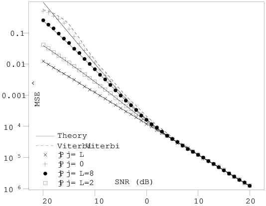
Refer to caption
Fig. 1: Phase error versus SNR for BPSK with L=4096L=4096.
Refer to caption
Fig. 2: Phase error versus SNR for QPSK with L=4096L=4096.
Refer to caption
Fig. 3: Phase error versus SNR for 88-PSK with L=4096L=4096.
Refer to caption
Fig. 4: Unbiased amplitude error versus SNR for BPSK.
Refer to caption
Fig. 5: Unbiased amplitude error versus SNR for QPSK.
Refer to caption
Fig. 6: Unbiased amplitude error versus SNR for 88-PSK.
Refer to caption
Fig. 7: Phase error versus SNR for QPSK.

IX Conclusion

We considered least squares estimators of carrier phase and amplitude from noisy communications signals that contain both pilot signals, known to the receiver, and data signals, unknown to the receiver. We focused on MM-ary phase shift keying constellations. The least squares estimator can be computed in O⁡(L​log⁡L)O(L\log L) operations using a modification of an algorithm due to Mackenthun [7], and is the maximum likelihood estimator in the case that the noise is additive white and Gaussian.

We showed, under some reasonably general conditions on the distribution of the noise, that the phase estimator θ^\hat{\theta} is strongly consistent and asymptotically normally distributed. However, the amplitude estimator ρ^0\hat{\rho}_{0} is biased, and converges to G⁡(0)​ρ0G(0)\rho_{0}. This bias is large when the signal to noise ratio is small. It would be interesting to investigate methods for correcting this bias. A method for estimating G⁡(0)G(0) at the receiver appears to be required.

Monte Carlo simulations were used to assess the performance of the least squares estimator and also to validate our asymptotic theory. Interestingly, when the SNR is small, it is counterproductive to use the data symbols to estimate the phase (Figure 7). This suggests the use of a weighted objective function, which would be an interesting topic for future research.

References

  • [1] R. G. McKilliam, Andre Pollok, Bill Cowley, Vaughan Clarkson, and Barry Quinn, “Noncoherent least squares estimators of carrier phase and amplitude,” submitted to IEEE Internat. Conf. Acoust. Spe. Sig. Process., Nov. 2012.
  • [2] A. Viterbi and A. Viterbi, “Nonlinear estimation of PSK-modulated carrier phase with application to burst digital transmission,” IEEE Trans. Inform. Theory, vol. 29, no. 4, pp. 543 – 551, Jul. 1983.
  • [3] W. G. Cowley, “Reference symbols can improve performance over differential coding in ML and near-ML detectors,” Signal Process., vol. 71, no. 1, pp. 95–99, Nov. 1998.
  • [4] S. G. Wilson, J. Freebersyser, and C. Marshall, “Multi-symbol detection of MPSK,” Proc. IEEE GLOBECOM, pp. 1692–1697, Nov. 1989.
  • [5] D. Makrakis and K. Feher, “Optimal noncoherent detection of PSK signals,” Electronics Letters, vol. 26, no. 6, pp. 398–400, Mar. 1990.
  • [6] J. Liu, J. Kim, S. C. Kwatra, and G. H. Stevens, “An analysis of the MPSK scheme with differential recursive detection (DRD),” Proc. IEEE Conf. on Veh. Tech., pp. 741–746, May 1991.
  • [7] K. M. Mackenthun, “A fast algorithm for multiple-symbol differential detection of MPSK,” IEEE Trans. Commun., vol. 42, pp. 1471–1474, Feb/Mar/Apr 1994.
  • [8] W. Sweldens, “Fast block noncoherent decoding,” IEEE Comms. Letters, vol. 5, no. 4, pp. 132–134, Apr. 2001.
  • [9] R. G. McKilliam, I. V. L. Clarkson, D. J. Ryan, and I. B. Collings, “Linear-time block noncoherent detection of PSK,” Proc. Internat. Conf. Acoust. Spe. Sig. Process., pp. 2465–2468, Apr. 2009.
  • [10] D. Divsalar and M. K. Simon, “Multi-symbol differential detection of MPSK,” IEEE Trans. Commun., vol. 38, no. 3, pp. 300–308, March 1990.
  • [11] M. Aydinlik and M. Salehi, “Turbo coded modulation for unequal error protection,” IEEE Trans. Commun., vol. 56, no. 4, pp. 555–564, Apr. 2008.
  • [12] S. Sandberg and N. Von Deetzen, “Design of bandwidth-efficient unequal error protection LDPC codes,” IEEE Trans. Commun., vol. 58, no. 3, pp. 802–811, Mar. 2010.
  • [13] P. Billingsley, Probability and measure, John Wiley & Sons, 1979.
  • [14] R. von Mises, “On the asymptotic distribution of differentiable statistical functions,” Annals of Mathematical Statistics, vol. 18, no. 3, pp. 309–348, Sep. 1947.
  • [15] A. W. van der Vaart, Asymptotic Statistics, Cambridge University Press, 1998.
  • [16] D. Pollard, “New ways to prove central limit theorems,” Econometric Theory, vol. 1, no. 3, pp. 295–313, Dec. 1985.
  • [17] D. Pollard, Convergence of Stochastic Processes, Springer-Verlag, New York, 1984.
  • [18] D. Pollard, “Asymptotics by empirical processes,” Statistical Science, vol. 4, no. 4, pp. 341–325, 1989.
  • [19] S.A. van de Geer, Empirical Processes in M-Estimation, Cambridge Series in Statistical and Probabilistic Mathematics. Cambridge University Press, 2009.
  • [20] R. G. McKilliam, B. G. Quinn, I. V. L. Clarkson, B. Moran, and B. Vellambi, “Polynomial phase estimation by phase unwrapping,” arxiv.org/abs/1211.0374, Nov 2012.
  • [21] P. Billingsley, Convergence of probability measures, John Wiley & Sons, 2nd edition, 1999.

-A Lemmas required for the proof of almost sure convergence (Theorem 1)

Lemma 1.

G⁡(λ^L)→G⁡(0)G(\hat{\lambda}_{L})\rightarrow G(0) almost surely as L→∞L\rightarrow\infty.

Proof:

Since G⁡(x)G(x) is uniquely maximised at x=0x=0,

0≤G⁡(0)−G⁡(λ^L),0\leq G(0)-G(\hat{\lambda}_{L}),

and since λ^L\hat{\lambda}_{L} is the maximiser of GL​(x)G_{L}(x),

0≤GL​(λ^L)−GL​(0).0\leq G_{L}(\hat{\lambda}_{L})-G_{L}(0).

Thus,

0\displaystyle 0 ≤G⁡(0)−G⁡(λ^L)\displaystyle\leq G(0)-G(\hat{\lambda}_{L})
≤G⁡(0)−G⁡(λ^L)+GL​(λ^L)−GL​(0)\displaystyle\leq G(0)-G(\hat{\lambda}_{L})+G_{L}(\hat{\lambda}_{L})-G_{L}(0)
≤|G⁡(0)−GL​(0)|+|GL​(λ^L)−G⁡(λ^L)|\displaystyle\leq|G(0)-G_{L}(0)|+|G_{L}(\hat{\lambda}_{L})-G(\hat{\lambda}_{L})|
≤2supλ∈[−π,π)|GL(λ)−G(λ)|,\displaystyle\leq 2\sup_{\lambda\in[-\pi,\pi)}{|G_{L}(\lambda)-G(\lambda)|},

and the last line converges almost surely to zero by Lemma 2. ∎

Lemma 2.

supλ∈[−π,π)|GL(λ)−G(λ)|→0\sup_{\lambda\in[-\pi,\pi)}{|G_{L}(\lambda)-G(\lambda)|}\rightarrow 0 almost surely as L→∞L\rightarrow\infty.

Proof:

Put TL​(λ)=𝔼​GL​(λ)T_{L}(\lambda)={\mathbb{E}}G_{L}(\lambda) and write

supλ∈[−π,π)|GL(λ)−G(λ)|\displaystyle\sup_{\lambda\in[-\pi,\pi)}{|G_{L}(\lambda)-G(\lambda)|}
=supλ∈[−π,π)|GL(λ)−TL(λ)+TL(λ)−G(λ)|\displaystyle=\sup_{\lambda\in[-\pi,\pi)}{|G_{L}(\lambda)-T_{L}(\lambda)+T_{L}(\lambda)-G(\lambda)|}
≤supλ∈[−π,π)|GL(λ)−TL(λ)|+supλ∈[−π,π)|TL(λ)−G(λ)|.\displaystyle\leq\sup_{\lambda\in[-\pi,\pi)}{|G_{L}(\lambda)-T_{L}(\lambda)|}+\sup_{\lambda\in[-\pi,\pi)}{|T_{L}(\lambda)-G(\lambda)|}.

Now,

TL​(λ)−G​(λ)\displaystyle T_{L}(\lambda)-G(\lambda) =(|P|L−p)​h1​(λ)+(|D|L−d)​h2​(λ)\displaystyle=\big(\tfrac{{\left|P\right|}}{L}-p\big)h_{1}(\lambda)+\big(\tfrac{{\left|D\right|}}{L}-d\big)h_{2}(\lambda)
=o⁡(1)​h1​(λ)+o⁡(1)​h2​(λ)\displaystyle=o(1)h_{1}(\lambda)+o(1)h_{2}(\lambda)

Since

|h1​(λ)|=|𝔼​R1​cos⁡(λ+Φ1)|≤𝔼​R1,{|h_{1}(\lambda)|}={|{\mathbb{E}}R_{1}\cos(\lambda+\Phi_{1})|}\leq{\mathbb{E}}R_{1},

and

|h2(λ)|=|𝔼R1cos⟨λ+Φ1⟩|≤𝔼R1{|h_{2}(\lambda)|}={|{\mathbb{E}}R_{1}\cos\left\langle\lambda+\Phi_{1}\right\rangle|}\leq{\mathbb{E}}R_{1}

for all λ∈[−π,π)\lambda\in[-\pi,\pi), it follows that

supλ∈[−π,π)|TL(λ)−G(λ)|≤o(1)𝔼R1→0\sup_{\lambda\in[-\pi,\pi)}{|T_{L}(\lambda)-G(\lambda)|}\leq o(1){\mathbb{E}}R_{1}\rightarrow 0

as L→∞L\rightarrow\infty. Lemma 3 shows that

supλ∈[−π,π)|GL(λ)−TL(λ)|→0\sup_{\lambda\in[-\pi,\pi)}{|G_{L}(\lambda)-T_{L}(\lambda)|}\rightarrow 0

almost surely as L→∞L\rightarrow\infty. ∎

Lemma 3.

Put TL​(λ)=𝔼​GL​(λ)T_{L}(\lambda)={\mathbb{E}}G_{L}(\lambda). Then

supλ∈[−π,π)|GL(λ)−TL(λ)|→0\sup_{\lambda\in[-\pi,\pi)}{|G_{L}(\lambda)-T_{L}(\lambda)|}\rightarrow 0

almost surely as L→∞L\rightarrow\infty.

Proof:

Put DL​(λ)=GL​(λ)−TL​(λ)D_{L}(\lambda)=G_{L}(\lambda)-T_{L}(\lambda) and let

λn=2​πN(n−1)−π,n=1,…,N\lambda_{n}=\tfrac{2\pi}{N}(n-1)-\pi,\qquad n=1,\dots,N

be NN points uniformly spaced on the interval [−π,π)[-\pi,\pi). Let Ln=[λn,λn+2​πN)L_{n}=[\lambda_{n},\lambda_{n}+\tfrac{2\pi}{N}) and observe that L1,…,LNL_{1},\dots,L_{N} partition [−π,π)[-\pi,\pi). Now

supλ∈[−π,π)\displaystyle\sup_{\lambda\in[-\pi,\pi)} |DL​(λ)|\displaystyle{|D_{L}(\lambda)|}
=supn=1,…,Nsupλ∈Ln|DL​(λ)−DL​(λn)+DL​(λn)|\displaystyle=\sup_{n=1,\dots,N}\sup_{\lambda\in L_{n}}{|D_{L}(\lambda)-D_{L}(\lambda_{n})+D_{L}(\lambda_{n})|}
≤UL+VL,\displaystyle\leq U_{L}+V_{L},

where

UL=supn=1,…,N|DL​(λn)|​andU_{L}=\sup_{n=1,\dots,N}{|D_{L}(\lambda_{n})|}\;\;\;\text{and}
VL=supn=1,…,Nsupλ∈Ln|DL​(λ)−DL​(λn)|.V_{L}=\sup_{n=1,\dots,N}\sup_{\lambda\in L_{n}}{|D_{L}(\lambda)-D_{L}(\lambda_{n})|}.

Lemma 4 shows that for any NN and ϵ>0\epsilon>0,

Pr{limL→∞UL>ϵ}=0,{\operatorname{Pr}}\left\{\lim_{L\rightarrow\infty}U_{L}>\epsilon\right\}=0,

that is, UL→0U_{L}\rightarrow 0 almost surely as L→∞L\rightarrow\infty. Lemma 5 shows that for any ϵ>0\epsilon>0,

Pr{limL→∞VL>ϵ+4​πN𝔼Ri}=0.{\operatorname{Pr}}\left\{\lim_{L\rightarrow\infty}V_{L}>\epsilon+\tfrac{4\pi}{N}{\mathbb{E}}R_{i}\right\}=0.

If we choose NN large enough that 4​π​𝔼​Ri<ϵ​N4\pi{\mathbb{E}}R_{i}<\epsilon N then

Pr\displaystyle{\operatorname{Pr}} {limL→∞supλ∈[−π,π)|DL(λ)|>3ϵ}\displaystyle\left\{\lim_{L\rightarrow\infty}\sup_{\lambda\in[-\pi,\pi)}{|D_{L}(\lambda)|}>3\epsilon\right\}
≤Pr{limL→∞(UL+VL)>3ϵ}\displaystyle\leq{\operatorname{Pr}}\left\{\lim_{L\rightarrow\infty}(U_{L}+V_{L})>3\epsilon\right\}
≤Pr{limL→∞(UL+VL)>ϵ+ϵ+4​πN𝔼Ri}\displaystyle\leq{\operatorname{Pr}}\left\{\lim_{L\rightarrow\infty}(U_{L}+V_{L})>\epsilon+\epsilon+\tfrac{4\pi}{N}{\mathbb{E}}R_{i}\right\}
≤Pr{limL→∞UL>ϵ}+Pr{limL→∞VL>ϵ+4​πN𝔼Ri}\displaystyle\leq{\operatorname{Pr}}\left\{\lim_{L\rightarrow\infty}U_{L}>\epsilon\right\}+{\operatorname{Pr}}\left\{\lim_{L\rightarrow\infty}V_{L}>\epsilon+\tfrac{4\pi}{N}{\mathbb{E}}R_{i}\right\}
=0.\displaystyle=0.

Thus supλ∈[−π,π)|DL(λ)|→0\sup_{\lambda\in[-\pi,\pi)}{|D_{L}(\lambda)|}\rightarrow 0 almost surely as L→∞L\rightarrow\infty. ∎

Lemma 4.

For any N>0N>0, UL→0U_{L}\rightarrow 0 almost surely as L→∞L\rightarrow\infty where ULU_{L} is defined in the proof of Lemma 3.

Proof:

Put

Zi​(λ)={Ri​cos⁡(λ+Φi),i∈PRicos⟨λ+Φi⟩,i∈DZ_{i}(\lambda)=\begin{cases}R_{i}\cos(\lambda+\Phi_{i}),&i\in P\\ R_{i}\cos\langle\lambda+\Phi_{i}\rangle,&i\in D\end{cases}

so that

DL​(λ)=GL​(λ)−TL​(λ)=1L​∑i∈P∪D(Zi​(λ)−𝔼​Zi​(λ)).D_{L}(\lambda)=G_{L}(\lambda)-T_{L}(\lambda)=\frac{1}{L}\sum_{i\in P\cup D}\big(Z_{i}(\lambda)-{\mathbb{E}}Z_{i}(\lambda)\big).

Now Z1​(λn),…,ZL​(λn)Z_{1}(\lambda_{n}),\dots,Z_{L}(\lambda_{n}) are independent with finite variance (because 𝔼​Ri2{\mathbb{E}}R_{i}^{2} is finite), so for each n=1,…,Nn=1,\dots,N,

|DL​(λn)|=|1L​∑i∈P∪D(Zi​(λn)−𝔼​Zi​(λn))|→0{\left|D_{L}(\lambda_{n})\right|}={\left|\frac{1}{L}\sum_{i\in P\cup D}\big(Z_{i}(\lambda_{n})-{\mathbb{E}}Z_{i}(\lambda_{n})\big)\right|}\rightarrow 0

almost surely as L→∞L\rightarrow\infty by Kolmogorov’s strong law of large numbers [13]. Thus

UL=supn=1,…,N|DL​(λn)|≤∑n=1N|DL​(λn)|→0U_{L}=\sup_{n=1,\dots,N}{|D_{L}(\lambda_{n})|}\leq\sum_{n=1}^{N}{|D_{L}(\lambda_{n})|}\rightarrow 0

almost surely to zero as L→∞L\rightarrow\infty. ∎

Lemma 5.

For any ϵ>0\epsilon>0,

Pr{limL→∞VL>ϵ+4​πN𝔼Ri}=0.{\operatorname{Pr}}\left\{\lim_{L\rightarrow\infty}V_{L}>\epsilon+\tfrac{4\pi}{N}{\mathbb{E}}R_{i}\right\}=0.
Proof:

Observe that

|DL​(λ)−DL​(λn)|\displaystyle{|D_{L}(\lambda)-D_{L}(\lambda_{n})|}
=|GL​(λ)−TL​(λ)−GL​(λn)+TL​(λn)|\displaystyle={\left|G_{L}(\lambda)-T_{L}(\lambda)-G_{L}(\lambda_{n})+T_{L}(\lambda_{n})\right|}
≤|GL​(λ)−GL​(λn)|+|𝔼​GL​(λ)−𝔼​GL​(λn)|\displaystyle\leq{\left|G_{L}(\lambda)-G_{L}(\lambda_{n})\right|}+{\left|{\mathbb{E}}G_{L}(\lambda)-{\mathbb{E}}G_{L}(\lambda_{n})\right|}
≤|GL​(λ)−GL​(λn)|+𝔼​|GL​(λ)−GL​(λn)|,\displaystyle\leq{\left|G_{L}(\lambda)-G_{L}(\lambda_{n})\right|}+{\mathbb{E}}{\left|G_{L}(\lambda)-G_{L}(\lambda_{n})\right|},

the last line following from Jensen’s inequality. Put

CL=supn=1,…,Nsupλ∈Ln|GL​(λ)−GL​(λn)|,C_{L}=\sup_{n=1,\dots,N}\sup_{\lambda\in L_{n}}{\left|G_{L}(\lambda)-G_{L}(\lambda_{n})\right|},

so that

VL\displaystyle V_{L} =supn=1,…,Nsupλ∈Ln|DL​(λ)−DL​(λn)|\displaystyle=\sup_{n=1,\dots,N}\sup_{\lambda\in L_{n}}{|D_{L}(\lambda)-D_{L}(\lambda_{n})|}
≤CL+supn=1,…,Nsupλ∈Ln𝔼​|GL​(λ)−GL​(λn)|\displaystyle\leq C_{L}+\sup_{n=1,\dots,N}\sup_{\lambda\in L_{n}}{\mathbb{E}}{\left|G_{L}(\lambda)-G_{L}(\lambda_{n})\right|}
≤CL+𝔼​CL,\displaystyle\leq C_{L}+{\mathbb{E}}C_{L},

where the last line follows because sup𝔼​|…|≤𝔼​sup|…|\sup{\mathbb{E}}|\dots|\leq{\mathbb{E}}\sup|\dots|. Lemma 6 shows that 𝔼​CL≤2​πN​𝔼​R1{\mathbb{E}}C_{L}\leq\tfrac{2\pi}{N}{\mathbb{E}}R_{1} and also that

Pr{limL→∞CL>ϵ+2​πN𝔼R1}=0.{\operatorname{Pr}}\left\{\lim_{L\rightarrow\infty}C_{L}>\epsilon+\tfrac{2\pi}{N}{\mathbb{E}}R_{1}\right\}=0.

Thus,

Pr\displaystyle{\operatorname{Pr}} {limL→∞VL>ϵ+4​πN𝔼R1}\displaystyle\left\{\lim_{L\rightarrow\infty}V_{L}>\epsilon+\tfrac{4\pi}{N}{\mathbb{E}}R_{1}\right\}
≤Pr{limL→∞(CL+𝔼CL)>ϵ+4​πN𝔼R1}\displaystyle\leq{\operatorname{Pr}}\left\{\lim_{L\rightarrow\infty}(C_{L}+{\mathbb{E}}C_{L})>\epsilon+\tfrac{4\pi}{N}{\mathbb{E}}R_{1}\right\}
≤Pr{limL→∞CL>ϵ+2​πN𝔼R1}=0.\displaystyle\leq{\operatorname{Pr}}\left\{\lim_{L\rightarrow\infty}C_{L}>\epsilon+\tfrac{2\pi}{N}{\mathbb{E}}R_{1}\right\}=0.

∎

Lemma 6.

The following statements hold:

  1. 1.

    𝔼​CL≤2​πN​𝔼​R1{\mathbb{E}}C_{L}\leq\tfrac{2\pi}{N}{\mathbb{E}}R_{1} for all positive integers LL,

  2. 2.

    for any ϵ>0\epsilon>0, Pr{limL→∞CL>ϵ+2​πN𝔼R1}=0{\operatorname{Pr}}\left\{\lim_{L\rightarrow\infty}C_{L}>\epsilon+\tfrac{2\pi}{N}{\mathbb{E}}R_{1}\right\}=0.

Proof:

If λ∈Ln\lambda\in L_{n}, then λ=λn+δ\lambda=\lambda_{n}+\delta with δ<2​πN\delta<\tfrac{2\pi}{N}, and from Lemma 7,

|cos⁡(λ+Φi)−cos⁡(λn+Φi)|≤2​πN,and\displaystyle{\left|\cos(\lambda+\Phi_{i})-\cos(\lambda_{n}+\Phi_{i})\right|}\leq\tfrac{2\pi}{N},\;\;\;\text{and}
|cos⁡⟨λ+Φi⟩−cos⁡⟨λn+Φi⟩|≤2​πN.\displaystyle{\left|\cos\langle\lambda+\Phi_{i}\rangle-\cos\langle\lambda_{n}+\Phi_{i}\rangle\right|}\leq\tfrac{2\pi}{N}.

Because these results do not depend on nn,

supn=1,…,Nsupλ∈Ln|Zi​(λ)−Zi​(λn)|≤Ri​2​πN\sup_{n=1,\dots,N}\sup_{\lambda\in L_{n}}{\left|Z_{i}(\lambda)-Z_{i}(\lambda_{n})\right|}\leq R_{i}\frac{2\pi}{N}

for all i=P∪Di=P\cup D. Also

CL\displaystyle C_{L} =supn=1,…,Nsupλ∈Ln|1L​∑i∈P∪DZi​(λ)−Zi​(λn)|\displaystyle=\sup_{n=1,\dots,N}\sup_{\lambda\in L_{n}}{\left|\frac{1}{L}\sum_{i\in P\cup D}Z_{i}(\lambda)-Z_{i}(\lambda_{n})\right|}
≤1L​∑i∈P∪Dsupn=1,…,Nsupλ∈Ln|Zi​(λ)−Zi​(λn)|\displaystyle\leq\frac{1}{L}\sum_{i\in P\cup D}\sup_{n=1,\dots,N}\sup_{\lambda\in L_{n}}{\left|Z_{i}(\lambda)-Z_{i}(\lambda_{n})\right|}
≤2​πN​L​∑i∈P∪DRi.\displaystyle\leq\frac{2\pi}{NL}\sum_{i\in P\cup D}R_{i}.

Thus,

𝔼​CL≤𝔼​2​πN​L​∑i∈P∪DRi=2​πN​𝔼​R1{\mathbb{E}}C_{L}\leq{\mathbb{E}}\frac{2\pi}{NL}\sum_{i\in P\cup D}R_{i}=\frac{2\pi}{N}{\mathbb{E}}R_{1}

and the first statement holds. Now,

2​πN​L​∑i∈P∪DRi→2​πN​𝔼​R1\frac{2\pi}{NL}\sum_{i\in P\cup D}R_{i}\rightarrow\frac{2\pi}{N}{\mathbb{E}}R_{1}

almost surely as L→∞L\rightarrow\infty by the strong law of large numbers, and so, for any ϵ>0\epsilon>0,

Pr\displaystyle{\operatorname{Pr}} {limL→∞CL>ϵ+2​πN𝔼R1}\displaystyle\left\{\lim_{L\rightarrow\infty}C_{L}>\epsilon+\tfrac{2\pi}{N}{\mathbb{E}}R_{1}\right\}
≤Pr{limL→∞2​πN​L∑i∈P∪DRi>ϵ+2​πN𝔼R1}=0.\displaystyle\leq{\operatorname{Pr}}\left\{\lim_{L\rightarrow\infty}\frac{2\pi}{NL}\sum_{i\in P\cup D}R_{i}>\epsilon+\tfrac{2\pi}{N}{\mathbb{E}}R_{1}\right\}=0.

∎

Lemma 7.

Let xx and δ\delta be real numbers. Then

|cos⁡(x+δ)−cos⁡(x)|≤|δ|,and\displaystyle{\left|\cos(x+\delta)-\cos(x)\right|}\leq{\left|\delta\right|},\;\;\;\text{and}
|cos⁡⟨x+δ⟩−cos⁡⟨x⟩|≤|δ|.\displaystyle{\left|\cos\left\langle x+\delta\right\rangle-\cos\left\langle x\right\rangle\right|}\leq{\left|\delta\right|}.
Proof:

Both cos⁡(x)\cos(x) and cos⁡⟨x⟩\cos\left\langle x\right\rangle are Lipschitz continuous functions from ℝ{\mathbb{R}} to ℝ{\mathbb{R}} with constant K=1K=1. That is, for any xx and yy in ℝ{\mathbb{R}},

|cos⁡(y)−cos⁡(x)|≤K​|x−y|=|x−y|,and\displaystyle{\left|\cos(y)-\cos(x)\right|}\leq K{\left|x-y\right|}={\left|x-y\right|},\;\;\;\text{and}
|cos⁡⟨y⟩−cos⁡⟨x⟩|≤K​|x−y|=|x−y|.\displaystyle{\left|\cos\left\langle y\right\rangle-\cos\left\langle x\right\rangle\right|}\leq K{\left|x-y\right|}={\left|x-y\right|}.

The lemma follows by putting y=x+δy=x+\delta. ∎

Lemma 8.

GL​(λ^L)→G⁡(0)G_{L}(\hat{\lambda}_{L})\rightarrow G(0) almost surely as L→∞L\rightarrow\infty.

Proof:

By the triangle inequality,

|GL​(λ^L)−G⁡(0)|≤|GL​(λ^L)−G⁡(λ^L)|+|G⁡(λ^L)−G⁡(0)|.{|G_{L}(\hat{\lambda}_{L})-G(0)|}\leq{|G_{L}(\hat{\lambda}_{L})-G(\hat{\lambda}_{L})|}+{|G(\hat{\lambda}_{L})-G(0)|}.

Now |GL​(λ^L)−G⁡(λ^L)|→0{|G_{L}(\hat{\lambda}_{L})-G(\hat{\lambda}_{L})|}\rightarrow 0 as L→∞L\rightarrow\infty as a result of Lemma 2, and |G⁡(λ^L)−G⁡(0)|→0{|G(\hat{\lambda}_{L})-G(0)|}\rightarrow 0 almost surely as L→∞L\rightarrow\infty because GG is continuous and λ^L→0\hat{\lambda}_{L}\rightarrow 0 almost surely as L→∞L\rightarrow\infty. ∎

-B Lemmas required for the proof of asymptotic normality (Theorem 2)

Lemma 9.

The derivative of GLG_{L} exists, and is equal to zero, at λ^L\hat{\lambda}_{L}. That is,

GL′​(λ^L)=d​GLd​λ​(λ^L)=0.G_{L}^{\prime}(\hat{\lambda}_{L})=\frac{dG_{L}}{d\lambda}(\hat{\lambda}_{L})=0.
Proof:

Observe that

GL(λ)=1L∑i∈PRicos(λ+Φi)+1L∑i∈DRicos⟨λ+Φi⟩G_{L}(\lambda)=\frac{1}{L}\sum_{i\in P}R_{i}\cos(\lambda+\Phi_{i})+\frac{1}{L}\sum_{i\in D}R_{i}\cos\langle\lambda+\Phi_{i}\rangle

is differentiable everywhere except when ⟨λ+Φi⟩=−πM\left\langle\lambda+\Phi_{i}\right\rangle=-\tfrac{\pi}{M} for any i∈Di\in D with Ri>0R_{i}>0. Let qiq_{i} be the smallest number from the interval [−πM,0][-\tfrac{\pi}{M},0] such that

sin⁡(qi)>−ρ0​|η|2​Ri4​L​ρ^​sin⁡(π/M)\sin(q_{i})>-\frac{\rho_{0}{|\eta|}^{2}R_{i}}{4L\hat{\rho}\sin(\pi/M)}

where η=e−j2π/M−1\eta=e^{-j2\pi/M}-1. Observe that qi<0q_{i}<0 when Ri>0R_{i}>0. Lemma 10 shows that

|⟨λ^L+Φi⟩|≤πM+qi{|\langle\hat{\lambda}_{L}+\Phi_{i}\rangle|}\leq\frac{\pi}{M}+q_{i}

for all i∈Di\in D. Thus, ⟨λ^L+Φi⟩≠−πM\langle\hat{\lambda}_{L}+\Phi_{i}\rangle\neq-\tfrac{\pi}{M} for i∈Di\in D such that Ri>0R_{i}>0 and therefore GLG_{L} is differentiable at λ^L\hat{\lambda}_{L}. That GL′​(λ^L)=0G_{L}^{\prime}(\hat{\lambda}_{L})=0 follows since λ^L\hat{\lambda}_{L} is a maximiser of GLG_{L}. ∎

Lemma 10.

Let qiq_{i} be defined as in Lemma 9. Then |⟨λ^L+Φi⟩|≤πM+qi{|\langle\hat{\lambda}_{L}+\Phi_{i}\rangle|}\leq\frac{\pi}{M}+q_{i} for all i∈Di\in D.

Proof:

Recall that {d^i=d^i​(θ^),i∈D}\{\hat{d}_{i}=\hat{d}_{i}(\hat{\theta}),i\in D\} defined in (8) are the minimisers of the function

S​S​({di,i∈D})=A−1L​|Y⁡({di,i∈D})|2,SS(\{d_{i},i\in D\})=A-\frac{1}{L}{|Y(\{d_{i},i\in D\})|}^{2},

defined in (6). The proof now proceeds by contradiction. Assume that

⟨λ^L+Φk⟩>πM+qk\langle\hat{\lambda}_{L}+\Phi_{k}\rangle>\frac{\pi}{M}+q_{k} (23)

for some k∈Dk\in D. Recalling the notation eke_{k} defined in Section II, put ri=d^i​ekr_{i}=\hat{d}_{i}e_{k}. We will show that

S​S​({ri,i∈D})<S​S​({d^i,i∈D}),SS(\{r_{i},i\in D\})<SS(\{\hat{d}_{i},i\in D\}),

violating the fact that {d^i,i∈D}\{\hat{d}_{i},i\in D\} are minimisers of S​SSS. First observe that,

Y⁡({ri,i∈D})=∑i∈Pyi​pi∗+∑i∈Dyi​r^i∗=Y^+η​yk​d^k∗,\displaystyle Y(\{r_{i},i\in D\})=\sum_{i\in P}y_{i}p_{i}^{*}+\sum_{i\in D}y_{i}\hat{r}_{i}^{*}=\hat{Y}+\eta y_{k}\hat{d}_{k}^{*},

where η=e−j2π/M−1\eta=e^{-j2\pi/M}-1 and Y^=Y⁡({d^i,i∈D})\hat{Y}=Y(\{\hat{d}_{i},i\in D\}). Now,

S​S\displaystyle SS ({ri,i∈D})\displaystyle(\{r_{i},i\in D\})
=A−1L​|Y⁡({ri,i∈D})|2\displaystyle=A-\frac{1}{L}{|Y(\{r_{i},i\in D\})|}^{2}
=A−1L​|Y^+η​yk​d^k∗|2\displaystyle=A-\frac{1}{L}{|\hat{Y}+\eta y_{k}\hat{d}_{k}^{*}|}^{2}
=A−1L​|Y^|2−2L​ℜ⁡(η​Y^∗​yk​d^k∗)−1L​|η​yk|2\displaystyle=A-\frac{1}{L}{|\hat{Y}|}^{2}-\frac{2}{L}\Re\left(\eta\hat{Y}^{*}y_{k}\hat{d}_{k}^{*}\right)-\frac{1}{L}{|\eta y_{k}|}^{2}
=S​S​({d^i,i∈D})−C,\displaystyle=SS(\{\hat{d}_{i},i\in D\})-C,

where

C=2L​ℜ⁡(η​Y^∗​yk​d^k∗)+1L​|η​yk|2.C=\frac{2}{L}\Re\left(\eta\hat{Y}^{*}y_{k}\hat{d}_{k}^{*}\right)+\frac{1}{L}{|\eta y_{k}|}^{2}.

Now 1L​Y^=a^=ρ^​ej​θ^\frac{1}{L}\hat{Y}=\hat{a}=\hat{\rho}e^{j\hat{\theta}} from (5) and using (19),

1L​Y^∗​yk​d^k∗=ρ^​ρ0​Rk​ej⁡⟨λ^L+Φk⟩,\frac{1}{L}\hat{Y}^{*}y_{k}\hat{d}_{k}^{*}=\hat{\rho}\rho_{0}R_{k}e^{j\langle\hat{\lambda}_{L}+\Phi_{k}\rangle},

so that

C=2​ρ^​ρ0​Rk​ℜ⁡(η​ej⁡⟨λ^L+Φk⟩)+1L​|η|2​ρ02​Rk2.C=2\hat{\rho}\rho_{0}R_{k}\Re\left(\eta e^{j\langle\hat{\lambda}_{L}+\Phi_{k}\rangle}\right)+\frac{1}{L}{|\eta|}^{2}\rho_{0}^{2}R_{k}^{2}. (24)

Let v=⟨λ^L+Φk⟩−πMv=\langle\hat{\lambda}_{L}+\Phi_{k}\rangle-\tfrac{\pi}{M} so that

η​ej⁡⟨λ^L+Φk⟩\displaystyle\eta e^{j\langle\hat{\lambda}_{L}+\Phi_{k}\rangle} =(e−j2π/M−1)ej​π/Mej​v\displaystyle=(e^{-j2\pi/M}-1)e^{j\pi/M}e^{jv}
=(e−jπ/M−ej​π/M)ej​v\displaystyle=(e^{-j\pi/M}-e^{j\pi/M})e^{jv}
=−2​j​sin⁡(πM)​ej​v,\displaystyle=-2j\sin(\tfrac{\pi}{M})e^{jv},

and

ℜ⁡(η​ej⁡⟨λ^L+Φk⟩)=2​sin⁡(πM)​sin⁡(v).\Re\left(\eta e^{j\langle\hat{\lambda}_{L}+\Phi_{k}\rangle}\right)=2\sin(\tfrac{\pi}{M})\sin(v).

Because we assumed (23), it follows that 0>v>qk0>v>q_{k} and, from the definition of qkq_{k},

−ρ0​|η|2​Rk4​L​ρ^​sin⁡(π/M)<sin⁡(v)<0.-\frac{\rho_{0}{|\eta|}^{2}R_{k}}{4L\hat{\rho}\sin(\pi/M)}<\sin(v)<0.

Substituting this into (24) gives C>0C>0, but then

S​S​({ri,i∈D})<S​S​({d^i,i∈D}),SS(\{r_{i},i\in D\})<SS(\{\hat{d}_{i},i\in D\}),

violating the fact that {d^i,i∈D}\{\hat{d}_{i},i\in D\} are minimisers of S​SSS. So (23) is false.

To show that ⟨λ^L+Φk⟩≥−πM−qk\langle\hat{\lambda}_{L}+\Phi_{k}\rangle\geq-\frac{\pi}{M}-q_{k} we use contradiction again. Assume that ⟨λ^L+Φk⟩<−πM−qk\langle\hat{\lambda}_{L}+\Phi_{k}\rangle<-\frac{\pi}{M}-q_{k}. Recalling the notation ek∗e_{k}^{*} defined in Section II, put ri=d^i​ek∗r_{i}=\hat{d}_{i}e_{k}^{*}. Now an analogous argument can be used to show that S​S​({ri,i∈D})<S​S​({d^i,i∈D})SS(\{r_{i},i\in D\})<SS(\{\hat{d}_{i},i\in D\}) again. ∎

Lemma 11.

Let QL​(λ)=𝔼​RL​(λ)−𝔼​RL​(0)Q_{L}(\lambda)={\mathbb{E}}R_{L}(\lambda)-{\mathbb{E}}R_{L}(0) where the function RLR_{L} is defined in (22). We have

L​QL​(λ^L)=L​λ^L​(p+H​d+oP​(1))\sqrt{L}Q_{L}(\hat{\lambda}_{L})=\sqrt{L}\hat{\lambda}_{L}\big(p+Hd+o_{P}(1)\big)

where p,dp,d and HH are defined in the statements of Theorems 1 and 2.

Proof:

We have

QL​(λ)=𝔼​RL​(λ)−𝔼​RL​(0)=|P|L​k1​(λ)+|D|L​k2​(λ)Q_{L}(\lambda)={\mathbb{E}}R_{L}(\lambda)-{\mathbb{E}}R_{L}(0)=\tfrac{{|P|}}{L}k_{1}(\lambda)+\tfrac{{|D|}}{L}k_{2}(\lambda)

where

k1​(λ)\displaystyle k_{1}(\lambda) =𝔼​R1​(sin⁡(λ+Φ1)−sin⁡(Φ1)),and\displaystyle={\mathbb{E}}R_{1}\big(\sin(\lambda+\Phi_{1})-\sin(\Phi_{1})\big),\;\;\;\text{and}
k2​(λ)\displaystyle k_{2}(\lambda) =𝔼​R1​(sin⁡⟨λ+Φ1⟩−sin⁡⟨Φ1⟩).\displaystyle={\mathbb{E}}R_{1}\big(\sin\left\langle\lambda+\Phi_{1}\right\rangle-\sin\left\langle\Phi_{1}\right\rangle\big). (25)

Lemma 12 shows that k1​(λ^L)=λ^L​(1+oP​(1))k_{1}(\hat{\lambda}_{L})=\hat{\lambda}_{L}\big(1+o_{P}(1)\big) and Lemma 13 shows that k2​(λ^L)=λ^L​(H+oP​(1))k_{2}(\hat{\lambda}_{L})=\hat{\lambda}_{L}\big(H+o_{P}(1)\big) and so

QL​(λ^L)\displaystyle Q_{L}(\hat{\lambda}_{L}) =|P|L​λ^L​(1+oP​(1))+|D|L​λ^L​(H+oP​(1))\displaystyle=\tfrac{{|P|}}{L}\hat{\lambda}_{L}\big(1+o_{P}(1)\big)+\tfrac{{|D|}}{L}\hat{\lambda}_{L}(H+o_{P}(1))
=λ^L​(|P|L+|D|L​H+oP​(1))\displaystyle=\hat{\lambda}_{L}\big(\tfrac{{|P|}}{L}+\tfrac{{|D|}}{L}H+o_{P}(1)\big)
=λ^L​(p+d​H+oP​(1)),\displaystyle=\hat{\lambda}_{L}\big(p+dH+o_{P}(1)\big),

since |P|L→p\frac{{|P|}}{L}\rightarrow p and |D|L→d\frac{{|D|}}{L}\rightarrow d as L→∞L\rightarrow\infty. The lemma follows by multiplying both sides of the above equation by L\sqrt{L}. ∎

Lemma 12.

Put

q1​(λ)+j​k1​(λ)=𝔼⁡[R1​ej⁡(λ+Φ1)−R1​ej​Φ1].q_{1}(\lambda)+jk_{1}(\lambda)={\mathbb{E}}\big[R_{1}e^{j(\lambda+\Phi_{1})}-R_{1}e^{j\Phi_{1}}\big].

We have q1​(λ)=λ^L​oP​(1)q_{1}(\lambda)=\hat{\lambda}_{L}o_{P}(1) and k1​(λ^L)=λ^L​(1+oP​(1))k_{1}(\hat{\lambda}_{L})=\hat{\lambda}_{L}\big(1+o_{P}(1)\big).

Proof:

We have

q1​(λ)+j​k1​(λ)=(ej​λ−1)​𝔼​R1​ej​Φ1=ej​λ−1q_{1}(\lambda)+jk_{1}(\lambda)=(e^{j\lambda}-1){\mathbb{E}}R_{1}e^{j\Phi_{1}}=e^{j\lambda}-1

since the mean of R1​ej​Φ1R_{1}e^{j\Phi_{1}} is 1. By a first order expansion about λ=0\lambda=0 we obtain

q1​(λ)+j​k1​(λ)=λ⁡(j+O⁡(λ))q_{1}(\lambda)+jk_{1}(\lambda)=\lambda\big(j+O(\lambda)\big)

Since λ^L\hat{\lambda}_{L} converges almost surely to zero as L→∞L\rightarrow\infty it follows that O⁡(λ^L)=oP​(1)O(\hat{\lambda}_{L})=o_{P}(1). Thus

q1​(λ^L)+j​k1​(λ^L)=λ^L​(j+oP​(1))q_{1}(\hat{\lambda}_{L})+jk_{1}(\hat{\lambda}_{L})=\hat{\lambda}_{L}\big(j+o_{P}(1)\big)

and the lemma follow by taking real and imaginary parts. ∎

Lemma 13.

Put

q2​(λ)+j​k2​(λ)=𝔼⁡[R1​ej​⟨λ+Φ1⟩−R1​ej​⟨Φ1⟩].q_{2}(\lambda)+jk_{2}(\lambda)={\mathbb{E}}\big[R_{1}e^{j\left\langle\lambda+\Phi_{1}\right\rangle}-R_{1}e^{j\left\langle\Phi_{1}\right\rangle}\big].

We have q2​(λ^L)=λ^L​oP​(1)q_{2}(\hat{\lambda}_{L})=\hat{\lambda}_{L}o_{P}(1) and k2​(λ^L)=λ^L​(H+oP​(1))k_{2}(\hat{\lambda}_{L})=\hat{\lambda}_{L}\big(H+o_{P}(1)\big) where HH is defined in the statement of Theorem 2.

Proof:

Because λ^L→0\hat{\lambda}_{L}\rightarrow 0 almost surely as L→∞L\rightarrow\infty, it is only the behaviour of q2​(λ)q_{2}(\lambda) and k2​(λ)k_{2}(\lambda) around λ=0\lambda=0 that is relevant. We will examine q2​(λ)q_{2}(\lambda) and k2​(λ)k_{2}(\lambda) for 0≤λ<πM0\leq\lambda<\tfrac{\pi}{M}. An analogous argument follows when −πM<λ<0-\tfrac{\pi}{M}<\lambda<0. To keep our notation clean put

ψk=2​πM​k+πM\psi_{k}=\frac{2\pi}{M}k+\frac{\pi}{M}

with k∈ℤk\in{\mathbb{Z}}. When Φ1∈[ψk−1,ψk−λ)\Phi_{1}\in[\psi_{k-1},\psi_{k}-\lambda),

ej​⟨λ+Φ1⟩−ej​⟨Φ1⟩\displaystyle e^{j\left\langle\lambda+\Phi_{1}\right\rangle}-e^{j\left\langle\Phi_{1}\right\rangle} =ej⁡(λ+Φ1−2​πM​k)−ej⁡(Φ1−2​πM​k)\displaystyle=e^{j\big(\lambda+\Phi_{1}-\tfrac{2\pi}{M}k\big)}-e^{j\big(\Phi_{1}-\tfrac{2\pi}{M}k\big)}
=(ej​λ−1)​ej⁡(Φ1−2​πM​k)\displaystyle=\big(e^{j\lambda}-1\big)e^{j\big(\Phi_{1}-\tfrac{2\pi}{M}k\big)}
=(ej​λ−1)​ej​⟨Φ1⟩,\displaystyle=\big(e^{j\lambda}-1\big)e^{j\left\langle\Phi_{1}\right\rangle},

and when Φ1∈[ψk−λ,ψk)\Phi_{1}\in[\psi_{k}-\lambda,\psi_{k}),

ej​⟨λ+Φ1⟩−\displaystyle e^{j\left\langle\lambda+\Phi_{1}\right\rangle}- ej​⟨Φ1⟩\displaystyle e^{j\left\langle\Phi_{1}\right\rangle}
=ej⁡(λ+Φ1−2​πM​k−2​πM)−ej⁡(Φ1−2​πM​k)\displaystyle=e^{j\big(\lambda+\Phi_{1}-\tfrac{2\pi}{M}k-\tfrac{2\pi}{M}\big)}-e^{j\big(\Phi_{1}-\tfrac{2\pi}{M}k\big)}
=(ej⁡(λ−2​πM)−1)​ej​⟨Φ1⟩\displaystyle=\big(e^{j\big(\lambda-\tfrac{2\pi}{M}\big)}-1\big)e^{j\left\langle\Phi_{1}\right\rangle}
=(ej​λ−1)​ej​⟨Φ1⟩+ej​λ​(e−j​2​πM−1)​ej​⟨Φ1⟩.\displaystyle=\big(e^{j\lambda}-1\big)e^{j\left\langle\Phi_{1}\right\rangle}+e^{j\lambda}\big(e^{-j\tfrac{2\pi}{M}}-1\big)e^{j\left\langle\Phi_{1}\right\rangle}.

Thus, when Φ1∈[ψk−1,ψk)\Phi_{1}\in[\psi_{k-1},\psi_{k}),

ej​⟨λ+Φ1⟩−ej​⟨Φ1⟩\displaystyle e^{j\left\langle\lambda+\Phi_{1}\right\rangle}-e^{j\left\langle\Phi_{1}\right\rangle} =(ej​λ−1)​ej​⟨Φ1⟩\displaystyle=\big(e^{j\lambda}-1\big)e^{j\left\langle\Phi_{1}\right\rangle}
+ej​λ​(e−j​2​πM−1)​ej​⟨Φ1⟩​χk​(Φ1,λ)\displaystyle\hskip 14.22636pt+e^{j\lambda}\big(e^{-j\tfrac{2\pi}{M}}-1\big)e^{j\left\langle\Phi_{1}\right\rangle}\chi_{k}(\Phi_{1},\lambda)

where

χk​(Φ1,λ)={1,Φ1∈[ψk−λ,ψk)0,otherwise.\chi_{k}(\Phi_{1},\lambda)=\begin{cases}1,&\Phi_{1}\in[\psi_{k}-\lambda,\psi_{k})\\ 0,&\text{otherwise}.\end{cases}

Now

q2​(λ)+j​k2​(λ)\displaystyle q_{2}(\lambda)+jk_{2}(\lambda) =𝔼⁡[R1​ej​⟨λ+Φ1⟩−R1​ej​⟨Φ1⟩]\displaystyle={\mathbb{E}}\big[R_{1}e^{j\left\langle\lambda+\Phi_{1}\right\rangle}-R_{1}e^{j\left\langle\Phi_{1}\right\rangle}\big]
=(ej​λ−1)​h2​(0)+ej​λ​B​(λ)\displaystyle=\big(e^{j\lambda}-1\big)h_{2}(0)+e^{j\lambda}B(\lambda) (26)

since 𝔼R1ej​⟨Φ1⟩=h2(0)+𝔼R1sin⟨Φ1⟩=h2(0){\mathbb{E}}R_{1}e^{j\left\langle\Phi_{1}\right\rangle}=h_{2}(0)+{\mathbb{E}}R_{1}\sin\left\langle\Phi_{1}\right\rangle=h_{2}(0) as a result of Lemma 15 and where

B⁡(λ)=(e−j​2​πM−1)​𝔼​R1​ej​⟨Φ1⟩​χ​(Φ1,λ)B(\lambda)=\big(e^{-j\tfrac{2\pi}{M}}-1\big){\mathbb{E}}R_{1}e^{j\left\langle\Phi_{1}\right\rangle}\chi(\Phi_{1},\lambda) (27)

and χ⁡(Φ1,λ)=∑k∈ℤχk​(Φ1,λ)\chi(\Phi_{1},\lambda)=\sum_{k\in{\mathbb{Z}}}\chi_{k}(\Phi_{1},\lambda).

Now ej​λ^L=1+oP​(1)e^{j\hat{\lambda}_{L}}=1+o_{P}(1) and ej​λ^L−1=λ^L​(j+oP​(1))e^{j\hat{\lambda}_{L}}-1=\hat{\lambda}_{L}\big(j+o_{P}(1)\big) by the argument in Lemma 12. Also

B⁡(λ^L)=−λ^L​(2​j​sin⁡(πM)​∑k=0M−1g⁡(ψk)+oP​(1))B(\hat{\lambda}_{L})=-\hat{\lambda}_{L}\left(2j\sin(\tfrac{\pi}{M})\sum_{k=0}^{M-1}g(\psi_{k})+o_{P}(1)\right)

by Lemma 14. Combining these results into (26) we obtain

q2​(λ)+\displaystyle q_{2}(\lambda)+ j​k2​(λ^L)\displaystyle jk_{2}(\hat{\lambda}_{L})
=λ^L​(j​h2​(0)−2​j​sin⁡(πM)​∑k=0M−1g⁡(ψk)+oP​(1))\displaystyle=\hat{\lambda}_{L}\left(jh_{2}(0)-2j\sin(\tfrac{\pi}{M})\sum_{k=0}^{M-1}g(\psi_{k})+o_{P}(1)\right)
=λ^L​(j​H+oP​(1))\displaystyle=\hat{\lambda}_{L}\big(jH+o_{P}(1)\big)

and the lemma follows by taking real and imaginary parts. ∎

Lemma 14.

With B⁡(λ)B(\lambda) defined in (27) we have

B⁡(λ^L)=−λ^L​(2​j​sin⁡(πM)​∑k=0M−1g⁡(ψk)+oP​(1))B(\hat{\lambda}_{L})=-\hat{\lambda}_{L}\left(2j\sin(\tfrac{\pi}{M})\sum_{k=0}^{M-1}g(\psi_{k})+o_{P}(1)\right)
Proof:

Put A⁡(λ)=𝔼​R1​ej​⟨Φ1⟩​χ​(Φ1,λ)A(\lambda)={\mathbb{E}}R_{1}e^{j\left\langle\Phi_{1}\right\rangle}\chi(\Phi_{1},\lambda). Recalling that f⁡(r,ϕ)f(r,\phi) is the joint pdf of R1R_{1} and Φ1\Phi_{1} we have

A⁡(λ)\displaystyle A(\lambda) =∫02​π∫0∞r​f​(r,ϕ)​ej​⟨ϕ⟩​χ​(ϕ,λ)​𝑑r​𝑑ϕ\displaystyle=\int_{0}^{2\pi}\int_{0}^{\infty}rf(r,\phi)e^{j\left\langle\phi\right\rangle}\chi(\phi,\lambda)drd\phi
=∑k∈ℤ∫02​πg⁡(ϕ)​ej​⟨ϕ⟩​χk​(ϕ,λ)​𝑑ϕ\displaystyle=\sum_{k\in{\mathbb{Z}}}\int_{0}^{2\pi}g(\phi)e^{j\left\langle\phi\right\rangle}\chi_{k}(\phi,\lambda)d\phi
=∑k=0M−1∫ψk−λψkg⁡(ϕ)​ej​⟨ϕ⟩​𝑑ϕ,\displaystyle=\sum_{k=0}^{M-1}\int_{\psi_{k}-\lambda}^{\psi_{k}}g(\phi)e^{j\left\langle\phi\right\rangle}d\phi,

the last line because the χk​(ϕ,λ)\chi_{k}(\phi,\lambda) terms inside the integral are zero for all ϕ∈[0,2​π]\phi\in[0,2\pi] when k∉{0,…,M−1}k\notin\{0,\dots,M-1\}. Observe that ⟨ϕ⟩→πM\left\langle\phi\right\rangle\rightarrow\tfrac{\pi}{M} as ϕ\phi approaches ψk\psi_{k} from below. Because g⁡(ψk)g(\psi_{k}) is continuous at ψk\psi_{k} for each k=0,…,M−1k=0,\dots,M-1 (by assumption in Theorem 2) we have

1λ​A​(λ)→∑k=0M−1g⁡(ψk)​ej​πM\frac{1}{\lambda}A(\lambda)\rightarrow\sum_{k=0}^{M-1}g(\psi_{k})e^{j\tfrac{\pi}{M}}

as λ\lambda approaches zero from above. We are only interested in the limit from above because we are working under the assumption that 0≤λ<πM0\leq\lambda<\frac{\pi}{M} (see the proof of Lemma 13). The analogous argument when −πM≤λ<0-\tfrac{\pi}{M}\leq\lambda<0 would involve limits as λ\lambda approaches zero from below. Thus

A⁡(λ^L)=λ^L​(ej​πM​∑k=0M−1g⁡(ψk)+oP​(1))A(\hat{\lambda}_{L})=\hat{\lambda}_{L}\left(e^{j\tfrac{\pi}{M}}\sum_{k=0}^{M-1}g(\psi_{k})+o_{P}(1)\right)

and the lemma follows since (e−j​2​πM−1)​ej​πM=−2​j​sin⁡(πM)\big(e^{-j\tfrac{2\pi}{M}}-1\big)e^{j\frac{\pi}{M}}=-2j\sin(\tfrac{\pi}{M}) and B⁡(λ)=(e−j​2​πM−1)​A​(λ)B(\lambda)=\big(e^{-j\tfrac{2\pi}{M}}-1\big)A(\lambda). ∎

Lemma 15.

𝔼R1sin⟨Φ1⟩=0{\mathbb{E}}R_{1}\sin\left\langle\Phi_{1}\right\rangle=0.

Proof:

Recalling that f⁡(r,ϕ)f(r,\phi) is the joint pdf of R1R_{1} and Φ1\Phi_{1} we have

𝔼R1sin⟨Φ1⟩\displaystyle{\mathbb{E}}R_{1}\sin\left\langle\Phi_{1}\right\rangle =∫02​π∫0∞rsin⟨ϕ⟩f(r,ϕ)drdϕ\displaystyle=\int_{0}^{2\pi}\int_{0}^{\infty}r\sin\left\langle\phi\right\rangle f(r,\phi)drd\phi
=∫−ππsin⟨ϕ⟩g(ϕ)dϕ.\displaystyle=\int_{-\pi}^{\pi}\sin\left\langle\phi\right\rangle g(\phi)d\phi.

The proof is immediate since g⁡(ϕ)g(\phi) is even and sin⁡⟨ϕ⟩\sin\left\langle\phi\right\rangle is odd. ∎

Lemma 16.

Let QL​(λ)=𝔼​RL​(λ)−𝔼​RL​(0)Q_{L}(\lambda)={\mathbb{E}}R_{L}(\lambda)-{\mathbb{E}}R_{L}(0) where the function RLR_{L} is defined in (22). Then,

L​(RL​(λ^L)−QL​(λ^L))=L​RL​(0)+oP​(1).\sqrt{L}\big(R_{L}(\hat{\lambda}_{L})-Q_{L}(\hat{\lambda}_{L})\big)=\sqrt{L}R_{L}(0)+o_{P}(1).
Proof:

Write

L​(RL​(λ^L)−QL​(λ^L))=WL​(λ^L)+L​RL​(0)\sqrt{L}\big(R_{L}(\hat{\lambda}_{L})-Q_{L}(\hat{\lambda}_{L})\big)=W_{L}(\hat{\lambda}_{L})+\sqrt{L}R_{L}(0)

where

WL​(λ)=L​(RL​(λ)−QL​(λ)−RL​(0))W_{L}(\lambda)=\sqrt{L}\big(R_{L}(\lambda)-Q_{L}(\lambda)-R_{L}(0)\big) (28)

is what is called an empirical process indexed by λ\lambda [18, 16, 19, 17]. Techniques from this literature can be used to show that for any δ>0\delta>0 and ν>0\nu>0, there exists ϵ>0\epsilon>0 such that

Pr{sup|λ|<ϵ|WL(λ)|>δ}<ν\Pr\left\{\sup_{{|\lambda|}<\epsilon}{|W_{L}(\lambda)|}>\delta\right\}<\nu

for all positive integers LL. This type of result is typically called tightness or asymptotic continuity [18, 19, 21]. We omit the proof which follows in a straightforward, but lengthy manner using an argument called symmetrisation followed by an argument called chaining [18, 19].

Since λ^L\hat{\lambda}_{L} converges almost surely to zero, it follows that for any ϵ>0\epsilon>0,

limL→∞Pr{|λ^L|≥ϵ}=0\lim_{L\rightarrow\infty}{\operatorname{Pr}}\left\{{|\hat{\lambda}_{L}|}\geq\epsilon\right\}=0

and therefore, for any ν>0\nu>0, Pr{|λ^L|≥ϵ}<ν{\operatorname{Pr}}\{{|\hat{\lambda}_{L}|}\geq\epsilon\}<\nu for all sufficiently large LL. Now

Pr\displaystyle{\operatorname{Pr}} {|WL(λ^L)|>δ}\displaystyle\left\{{|W_{L}(\hat{\lambda}_{L})|}>\delta\right\}
=Pr{|WL(λ^L)|>δand|λ^L|<ϵ}\displaystyle={\operatorname{Pr}}\left\{{|W_{L}(\hat{\lambda}_{L})|}>\delta\;\text{and}\;{|\hat{\lambda}_{L}|}<\epsilon\right\}
+Pr{|WL(λ^L)|>δand|λ^L|≥ϵ}\displaystyle\hskip 19.91684pt+{\operatorname{Pr}}\left\{{|W_{L}(\hat{\lambda}_{L})|}>\delta\;\text{and}\;{|\hat{\lambda}_{L}|}\geq\epsilon\right\}
≤Pr{sup|λ|<ϵ|WL(λ)|>δ}+Pr{|λ^L|≥ϵ}\displaystyle\leq{\operatorname{Pr}}\left\{\sup_{{|\lambda|}<\epsilon}{|W_{L}(\lambda)|}>\delta\right\}+{\operatorname{Pr}}\left\{{|\hat{\lambda}_{L}|}\geq\epsilon\right\}
≤2​ν,\displaystyle\leq 2\nu,

for all sufficiently large LL. Since ν\nu and δ\delta can be chosen arbitrarily small, it follows that WL​(λ^L)W_{L}(\hat{\lambda}_{L}) converges in probability to zero as N→∞N\rightarrow\infty. ∎

Lemma 17.

The distribution of L​RL​(0)\sqrt{L}R_{L}(0) converges to the normal with zero mean and variance p​A1+d​A2pA_{1}+dA_{2} as L→∞L\rightarrow\infty.

Proof:

Observe that L​RL​(0)=CL+DL\sqrt{L}R_{L}(0)=C_{L}+D_{L} where

CL=1L∑i∈PRisin(Φi),DL=1L∑i∈DRisin⟨Φi⟩.C_{L}=\frac{1}{\sqrt{L}}\sum_{i\in P}R_{i}\sin(\Phi_{i}),\qquad D_{L}=\frac{1}{\sqrt{L}}\sum_{i\in D}R_{i}\sin\langle\Phi_{i}\rangle.

From the standard central limit theorem the distribution of CLC_{L} converges to the normal with mean p​𝔼​R1​sin⁡(Φ1)=0\sqrt{p}{\mathbb{E}}R_{1}\sin(\Phi_{1})=0 as a result of (16), and variance

p​A1=p​𝔼​R12​sin2⁡(Φ1).pA_{1}=p{\mathbb{E}}R_{1}^{2}\sin^{2}(\Phi_{1}).

Similarly, the distribution of DLD_{L} converges to the normal with mean d𝔼R1sin⟨Φ1⟩=0\sqrt{d}{\mathbb{E}}R_{1}\sin\left\langle\Phi_{1}\right\rangle=0 as a result of Lemma 15, and variance

d​A2=d​𝔼​R12​sin2⁡⟨Φ1⟩.dA_{2}=d{\mathbb{E}}R_{1}^{2}\sin^{2}\left\langle\Phi_{1}\right\rangle.

The lemma holds because CLC_{L} and DLD_{L} are independent. ∎

Lemma 18.

Let TL​(λ)=𝔼​GL​(λ)T_{L}(\lambda)={\mathbb{E}}G_{L}(\lambda). We have

L​(GL​(λ^L)−TL​(λ^L))=XL+oP​(1),\sqrt{L}\big(G_{L}(\hat{\lambda}_{L})-T_{L}(\hat{\lambda}_{L})\big)=X_{L}+o_{P}(1),

where XL=L​(GL​(0)−TL​(0))X_{L}=\sqrt{L}\big(G_{L}(0)-T_{L}(0)\big).

Proof:

Write

L​(GL​(λ^L)−TL​(λ^L))=YL​(λ^L)+XL\sqrt{L}\big(G_{L}(\hat{\lambda}_{L})-T_{L}(\hat{\lambda}_{L})\big)=Y_{L}(\hat{\lambda}_{L})+X_{L}

where

YL​(λ)=L​(GL​(λ)−TL​(λ))−XL.Y_{L}(\lambda)=\sqrt{L}\big(G_{L}(\lambda)-T_{L}(\lambda)\big)-X_{L}. (29)

is an empirical process indexed by λ\lambda, similar to WLW_{L} from (28). As with WLW_{L} results from the literature on empirical processes can be used to show that for any δ>0\delta>0 and ν>0\nu>0, there exists ϵ>0\epsilon>0 such that

Pr{sup|λ|<ϵ|YL(λ)|>δ}<ν.\Pr\left\{\sup_{{|\lambda|}<\epsilon}{|Y_{L}(\lambda)|}>\delta\right\}<\nu.

The proof now follows by an argument analogous to that in Lemma 16. ∎

Lemma 19.

L​(TL​(λ^L)−G⁡(0))=oP​(1)\sqrt{L}\big(T_{L}(\hat{\lambda}_{L})-G(0)\big)=o_{P}(1).

Proof:

The argument is similar to that used in Lemma 11. First observe that

TL​(λ)\displaystyle T_{L}(\lambda) =|P|L𝔼R1cos(λ+Φ1)+|D|L𝔼R1cos⟨λ+Φ1⟩\displaystyle=\frac{{|P|}}{L}{\mathbb{E}}R_{1}\cos(\lambda+\Phi_{1})+\frac{{|D|}}{L}{\mathbb{E}}R_{1}\cos\left\langle\lambda+\Phi_{1}\right\rangle
=(p+o(L−1/2))𝔼R1cos(λ+Φ1)\displaystyle=\big(p+o(L^{-1/2})\big){\mathbb{E}}R_{1}\cos(\lambda+\Phi_{1})
+(d+o(L−1/2))𝔼R1cos⟨λ+Φ1⟩,\displaystyle\hskip 56.9055pt+\big(d+o(L^{-1/2})\big){\mathbb{E}}R_{1}\cos\left\langle\lambda+\Phi_{1}\right\rangle,

and because |P|L=p+o(L−1/2)\tfrac{{\left|P\right|}}{L}=p+o(L^{-1/2}) and |D|L=d+o(L−1/2)\tfrac{{\left|D\right|}}{L}=d+o(L^{-1/2}) (by assumption in Theorem 2), we have

L​(TL​(λ)−G⁡(0))=L​p​q1​(λ)+L​d​q2​(λ)+o⁡(1),\displaystyle\sqrt{L}\big(T_{L}(\lambda)-G(0)\big)=\sqrt{L}pq_{1}(\lambda)+\sqrt{L}dq_{2}(\lambda)+o(1),

where

q1​(λ)\displaystyle q_{1}(\lambda) =𝔼​R1​(cos⁡(λ+Φ1)−cos⁡(Φ1))​and\displaystyle={\mathbb{E}}R_{1}\big(\cos(\lambda+\Phi_{1})-\cos(\Phi_{1})\big)\;\;\;\text{and}
q2​(λ)\displaystyle q_{2}(\lambda) =𝔼​R1​(cos⁡⟨λ+Φ1⟩−cos⁡⟨Φ1⟩).\displaystyle={\mathbb{E}}R_{1}\big(\cos\left\langle\lambda+\Phi_{1}\right\rangle-\cos\left\langle\Phi_{1}\right\rangle\big). (30)

Lemma 12 shows that q1​(λ^L)=λ^L​oP​(1)q_{1}(\hat{\lambda}_{L})=\hat{\lambda}_{L}o_{P}(1) and Lemma 13 shows that q2​(λ^L)=λ^L​oP​(1)q_{2}(\hat{\lambda}_{L})=\hat{\lambda}_{L}o_{P}(1) and so

L​(TL​(λ)−G⁡(0))=L​λ^L​oP​(1)+o⁡(1).\sqrt{L}\big(T_{L}(\lambda)-G(0)\big)=\sqrt{L}\hat{\lambda}_{L}o_{P}(1)+o(1).

The lemma follows since L​λ^L\sqrt{L}\hat{\lambda}_{L} converges in distribution. ∎

Lemma 20.

The distribution of

XL=L​(GL​(0)−TL​(0))=L​(GL​(0)−𝔼​GL​(0))X_{L}=\sqrt{L}\big(G_{L}(0)-T_{L}(0)\big)=\sqrt{L}\big(G_{L}(0)-{\mathbb{E}}G_{L}(0)\big)

converges, as L→∞L\rightarrow\infty, to the normal with zero mean and covariance p​B1+d​B2.pB_{1}+dB_{2}.

Proof:

Observe that XL=CL′+DL′X_{L}=C_{L}^{\prime}+D_{L}^{\prime} where

CL′=1L​∑i∈P(Ri​cos⁡(Φi)−h1​(0)),C_{L}^{\prime}=\frac{1}{\sqrt{L}}\sum_{i\in P}\big(R_{i}\cos(\Phi_{i})-h_{1}(0)\big),
DL′=1L∑i∈D(Ricos⟨Φi⟩−h2(0)),D_{L}^{\prime}=\frac{1}{\sqrt{L}}\sum_{i\in D}(R_{i}\cos\left\langle\Phi_{i}\right\rangle-h_{2}(0)),

where h1h_{1} and h2h_{2} are defined in the statement of Theorem 1. From the standard central limit theorem the distribution of CL′C_{L}^{\prime} converges to the normal with zero mean and variance

p​B1=p​𝔼​R12​cos2⁡(Φ1)−p​h12​(0)=p​𝔼​R12​cos2⁡(Φ1)−ppB_{1}=p{\mathbb{E}}R_{1}^{2}\cos^{2}(\Phi_{1})-ph_{1}^{2}(0)=p{\mathbb{E}}R_{1}^{2}\cos^{2}(\Phi_{1})-p

since h1​(0)=1h_{1}(0)=1. Similarly the distribution of DL′D_{L}^{\prime} converges to the normal with zero mean and variance

d​B2=d​𝔼​R12​cos2⁡⟨Φ1⟩−d​h22​(0).dB_{2}=d{\mathbb{E}}R_{1}^{2}\cos^{2}\left\langle\Phi_{1}\right\rangle-dh_{2}^{2}(0).

The lemma follows since CL′C_{L}^{\prime} and DL′D_{L}^{\prime} are independent. ∎