∎
Maximum likelihood estimation in constrained parameter spaces for mixtures of factor analyzers
Abstract
Mixtures of factor analyzers are becoming more and more popular in the area of model based clustering of high-dimensional data. According to the likelihood approach in data modeling, it is well known that the unconstrained log-likelihood function may present spurious maxima and singularities and this is due to specific patterns of the estimated covariance structure, when their determinant approaches 0. To reduce such drawbacks, in this paper we introduce a procedure for the parameter estimation of mixtures of factor analyzers, which maximizes the likelihood function in a constrained parameter space. We then analyze and measure its performance, compared to the usual non-constrained approach, via some simulations and applications to real data sets.
Keywords:
Constrained estimation Factor Analyzers Modeling Mixture Models Model-Based Clustering.1 Introduction and motivation
Finite mixture distributions have been receiving a growing interest in statistical modeling. Their central role is mainly due to their double nature: they combine the flexibility of non-parametric models with the strong and useful mathematical properties of parametric models. According to this approach, when we know that a sample of observations has been drawn from different populations, we assume a specific distributional form in each of the underlying populations. The purpose is to decompose the sample into its mixture components, which, for quantitative data, are usually modeled as a multivariate Gaussian distribution, and to estimate parameters. The assumption of underlying normality, besides the elegant analytic properties, allows also to employ the EM algorithm for the ML estimation of the parameters. On the other side, when considering a large number of observed variables, Gaussian mixture models can provide an over-parameterized solution as, besides the mixing weights, it is required to estimate the mean vector and the covariance matrix for each component (Peel and McLachlan, 2000). As a consequence, we observe at the same time an undue load of computationally intensive procedures for the estimation.
This is the reason why a number of strategies have been introduced in the literature to avoid over-parameterized solutions. Among the various proposal, some authors developed methodologies for variable selection (see, f.i., Liu et al. (2003) and Hoff (2005) in the Bayesian framework, Pan and Shen (2007) and Raftery and Dean (2006) in the frequentist one). They further motivate their approach from the observation that the presence of non-informative variables can be strongly misleading for some clustering methods. With the same purpose of parsimony, but a completely different approach, Banfield and Raftery (1993) devised a methodology to identify common patterns among the component-covariance matrices; their proposal arose a great attention in the literature. Along a slightly different line of thinking, Ghahramani and Hilton (1997) and McLachlan et al. (2003) proposed to employ latent variables to perform dimensional reduction in each component, starting from the consideration that in many phenomena some few unobserved features could be explained by the many observed ones.
In this paper we address mixtures of factor analyzers by assuming that the data have been generated by a linear factor model with latent variables modeled as Gaussian mixtures. Our purpose is to improve the performances of the EM algorithm, by facing with some of its issues and giving practical recipes to overcome them. It is well known that the EM algorithm generates a sequence of estimates, starting from an initial guess, so that the corresponding sequence of the log-likelihood values is not decreasing. However, the convergence toward the MLE is not guaranteed, because the log-likelihood is unbounded and presents local maxima. Another critical point is that the parameter estimates as well as the convergence of the whole estimation process may be affected by the starting values (see, f.i., McLachlan and Krishnan (2007)) so that the final estimate crucially depends on the initial guess. This issue has been investigated by many authors, starting from the seminal paper of Redner and Walker (1984). Along the lines of (Ingrassia, 2004), in this paper we introduce and implement a procedure for the parameters estimation of mixtures of factor analyzers, which maximizes the likelihood function in a constrained parameter space, having no singularities and a reduced number of spurious local maxima. We then analyze and measure its performance, compared to the usual non-constrained approach.
We have organized the rest of the paper as follows. In Section 2 we summarize main ideas about Gaussian Mixtures of Factor Analyzer model; in Section 3 we provide fairly extensive notes concerning the likelihood function and the AECM algorithm. Some well known considerations (Hathaway, 1985) related to spurious maximizers and singularities in the EM algorithm are recalled in Section 4, and motivate our proposal to introduce constraints on factor analyzers. Further, we give a detailed methodology to implement such constraints into the EM algorithm. In Section 6 we show and discuss the improved performance of our procedure, on the ground of some numerical results based on both simulated and real data. Section 7 contains concluding notes and provides ideas for future research.
2 The Gaussian Mixture of Factor analyzers
Within the Gaussian Mixture (GM) model-based approach to density estimation and clustering, the density of the -dimensional random variable of interest is modelled as a mixture of a number, say , of multivariate normal densities in some unknown proportions . That is, each data point is taken to be a realization of the mixture probability density function,
| (1) |
where denotes the -variate normal density function with mean and covariance matrix . Here the vector of unknown parameters consists of the mixing proportions , the elements of the component means , and the distinct elements of the component-covariance matrices . Therefore, the -component normal mixture model (1) with unrestricted component-covariance matrices is a highly parametrized model. We crucially need some method for parsimonious parametrization of the matrices , because they requires parameters. Among the various proposals for dimensionality reduction, we are interested here in considering Mixtures of Gaussian Factor Analyzers (MGFA), which allows to explain data by explicitly modeling correlations between variables in multivariate observations. We postulate a finite mixture of linear sub-models for the distribution of the full observation vector , given the (unobservable) factors . That is we can provide a local dimensionality reduction method by assuming that the distribution of the observation can be given as
| (2) |
where is a matrix of factor loadings, the factors are distributed independently of the errors , which are independently distributed, and is a diagonal matrix . We suppose that , which means that unobservable factors are jointly explaining the observable features of the statistical units. Under these assumptions, the mixture of factor analyzers model is given by (1), where the -th component-covariance matrix has the form
| (3) |
The parameter vector now consists of the elements of the component means , the , and the , along with the mixing proportions , on putting . Note that in the case of , there is an infinity of choices for , since model (2) is still satisfied if we replace by , where is any orthogonal matrix of order . As constraints are needed for to be uniquely defined, the number of free parameters, for each component of the mixture, is
Comparing the two approaches and willing now to measure the gained parsimony when we use mixtures of factor analyzers, with respect to the more usual gaussian mixtures, and denoting by and , the number of the estimated parameters for the covariance matrices in the GM and MGFA models, respectively, we have to choose values of such that the following quantity is positive
i.e.:
This is the only requirement for parsimony. Now, we can express the relative reduction given by
In Table 1 we report the relative reduction, in term of lower number of estimated parameters for the covariance matrices in the MGFA models, with respect to the GM models.
| 1 | 2 | 3 | 4 | 5 | 6 | 7 | 8 | 9 | 10 | 11 | 12 | 13 | 14 | 15 | |
|---|---|---|---|---|---|---|---|---|---|---|---|---|---|---|---|
| 1 | - | - | - | 0.20 | 0.33 | 0.43 | 0.50 | 0.56 | 0.60 | 0.64 | 0.67 | 0.69 | 0.71 | 0.73 | 0.75 |
| 2 | - | - | - | - | 0.07 | 0.19 | 0.29 | 0.36 | 0.42 | 0.47 | 0.52 | 0.55 | 0.58 | 0.61 | 0.63 |
| 3 | - | - | - | - | - | - | 0.11 | 0.19 | 0.27 | 0.33 | 0.38 | 0.42 | 0.46 | 0.50 | 0.53 |
| 4 | - | - | - | - | - | - | - | 0.06 | 0.13 | 0.20 | 0.26 | 0.31 | 0.35 | 0.39 | 0.43 |
| 5 | - | - | - | - | - | - | - | - | 0.02 | 0.09 | 0.15 | 0.21 | 0.25 | 0.30 | 0.33 |
The relative reduction represents the extent to which the factor model offers a simpler interpretation for the behaviour of than the alternative assumption given by the gaussian mixture model.
3 The likelihood function and the EM algorithm for MGFA
In this section we summarize the main steps of the EM algorithm for mixtures of Factor analyzers, see e.g. McLachlan and Peel (2000) for details.
Let be a sample of size from density (1), and let () denotes the realization of in (2). For given data , parameters in (1) can be estimated according to the likelihood approach via the EM algorithm, where the likelihood function is given by:
where we set (). Consider the augmented data , where , with if comes from the -th population and otherwise. Then, the complete-data likelihood function can be written in the form:
| (4) |
In particular, due to the factor structure of the model, see Meng and van Dyk (1997), we have to consider the alternating expectation-conditional maximization (AECM) algorithm. Such a procedure is an extension of the EM algorithm that uses different specifications of missing data at each stage. The idea is to partition in such a way that is easy to maximize for given and vice versa. Then, we can iterate between these two conditional maximizations until convergence. In this case where the missing data are the unobserved group labels , and the second part of the parameters vector is given by where the missing data are the group labels and the unobserved latent factors . Hence, the application of the AECM algorithm consists of two cycles, and there is one E-step and one CM-step alternatively considering and in each pair of cycles.
First Cycle.
Here it is where the missing data are the unobserved group labels . The complete data likelihood is
| (5) |
The E-step on the first cycle on the -th iteration requires the calculation of which is the expected complete-data log-likelihood given the data and using the current estimate for . In practice it requires calculating and usual computations show that this step is achieved by replacing each by its current conditional expectation given the observed data , that is we replace by , where
| (6) |
On the M-step, the maximization of this complete-data log-likelihood yields
where . According to notation in McLachlan and Peel (2000), we set .
Second Cycle.
Here it is , where the missing data are the unobserved group labels and the latent factors . Therefore, the complete data likelihood is
| (7) |
where
Now the complete data log-likelihood is given by
| (8) |
Some algebras lead to the following estimate of , :
where we set
Hence the maximum likelihood estimates and for and can be obtained by alternatively computing the update estimates and , by
| (9) |
and, from the latter, evaluating the update estimates and by
| (10) |
iterating these two steps until convergence on and , so giving and .
In summary, the procedure can be described as follows. For a given initial random clustering , on the iteration, the algorithm carries out the following steps, for :
- 1.
Compute and consequently obtain , , and ;
- 2.
Set a starting value for and from ;
- 3.
Repeat the following steps, until convergence on and :
- (a)
Compute and from (10);
- (b)
Set and ;
- (c)
Compute and ;
- (d)
Set and ;
- (a)
To completely describe the algorithm, here we give more details on how to specify the starting values for and from , as it is needed in Step 2.
Starting from the eigen-decomposition of , say , computed on the base of , the main idea is that has to synthesize the ”more important” relations between the observed features, see McNicholas and Murphy (2008). Then, looking at the equality , the initial values of were set as
| (11) |
where is the th largest eigenvalue of and is the th element of the corresponding eigenvector (the th column in ), for and . Finally the matrices can be initialized by the position .
4 Likelihood maximization in constrained parametric spaces
Properties of maximum likelihood estimation for normal mixture models have been deeply investigated. It is well known that is unbounded on and may present many local maxima. Day (1969) was perhaps the first noting that any small number of sample points, grouped sufficiently close together, can give raise to spurious maximizers, corresponding to parameters points with greatly differing component standard deviation. To overcome this issue and to prevent from singularities, Hathaway (1985) proposed a constrained maximum likelihood formulation for mixtures of univariate normal distributions, suggesting a natural extension to the multivariate case. Let , then the following constraints
| (12) |
on the eigenvalues of leads to properly defined, scale-equivariant, consistent ML-estimators for the mixture-of-normal case, see Hennig (2004). It is easy to show that a sufficient condition for (12) is
| (13) |
where denotes the th eigenvalue of i.e. , and for such that , see Ingrassia (2004). Differently from (12), condition (13) can be easily implemented in any optimization algorithm. Let us consider the constrained parameter space of :
| (14) |
Due to the structure of the covariance matrix given in (3), bound in (13) yields
| (15) |
where and denote the smallest and the largest eigenvalue of respectively. Since and are symmetric and positive definite, then it results:
| (16) | ||||
| (17) |
see Lütkepohl (1996). Moreover, being a diagonal matrix, then
| (18) |
where denotes the -th diagonal entry of the matrix .
Concerning the square matrix (), we can get its eigenvalue decomposition, i.e. we can find and such that
| (19) |
where is the orthonormal matrix whose rows are the eigenvectors of and is the diagonal matrix of the eigenvalues of , sorted in non increasing order, i.e. , and .
Now, we can apply the singular value decomposition to the rectangular matrix , so giving , where is a unitary matrix (i.e., such that ) and is a rectangular diagonal matrix with nonnegative real numbers on the diagonal, known as singular values, and is a unitary matrix. The columns of and the columns of are called the left singular vectors and right singular vectors of , respectively. Now we have that
| (20) |
and equating (19) and (20) we get and , that is
| (21) |
with . In particular, it is known that only the first values of are non negative, and the remaining terms are null. Thus it results
| (22) |
5 Constraints on the covariance matrix for factor analyzers
The two-fold (eigenvalue and singular value) decomposition of the presented above, suggests how to modify the EM algorithm in such a way that the eigenvalues of the covariances (for ) are confined into suitable ranges. To this aim we have to implement constraints (23), (24) and (25).
We proceed as follows on the th iteration:
- 1.
Decompose according to the singular value decomposition as ;
- 2.
Compute the squared singular values of ;
- 3.
Create a copy of and a copy of ;
- 4.
For to , if , then if set else into ;
- 5.
For to , if then set into ;
- 6.
For to , if , then if set into else into ;
- 7.
For to , if then set into ;
- 8.
Set ;
- 9.
Set .
- 10.
Stop.
It is important to remark that the resulting EM algorithm is monotone, once the initial guess, say , satisfies the constraints. Further, as shown in the case of gaussian mixtures in Ingrassia and Rocci (2007), the maximization of the complete loglikelihood is guaranteed. From the other side, it is apparent that the above recipes require some a priori information on the covariance structure of the mixture, throughout the bounds and .
6 Numerical studies
In this section we present numerical studies, based on both simulated and real data sets, in order to show the performance of the constrained EM algorithm with respect to unconstrained approaches.
6.1 Artificial data
We consider here three mixtures of components of -variate normal distributions, for different values of the parameter . First, we point out that the point of local maximum corresponding to the consistent estimator , has been chosen to be the limit of the EM algorithm using the true parameter as initial estimate, i.e. considering the true classification. In other words, we set if the th unit comes from the th component and otherwise. In the following, such estimate will be referred to as the right maximum of the likelihood function.
To begin with, we generate a set of 100 different random initial clusterings to initialize the algorithm at each run. To this aim, for a fixed number of components of the mixture, we draw each time a set of random starting values for the from the multinomial distribution with values in with parameters . Then we run a hundred times both the unconstrained and the constrained AECM algorithms (for different values of the constraints ) using the same set of initial clusterings in both cases. The initial values for the elements of and can be obtained as described at the end of Section 3 from the eigen-decomposition of , and the algorithms run until convergence or it reaches the fixed maximum number of iterations.
The stopping criterion is based on the Aitken acceleration procedure (Aitken, 1926), to estimate the asymptotic maximum of the log-likelihood at each iteration of the EM algorithm (in such a way, a decision can be made regarding whether or not the algorithm reaches convergence; that is, whether or not the log-likelihood is sufficiently close to its estimated asymptotic value). The Aitken acceleration at iteration is given by
where , , and are the log-likelihood values from iterations , , and , respectively. Then, the asymptotic estimate of the log-likelihood at iteration is given by
see Böhning et al. (1994). In our analyses, the algorithms stop when , with . Programs have been written in the R language; the different cases and the obtained results are described below.
Mixture 1: , , , .
The sample has been generated with weights according to the following parameters:
Hence, the covariance matrices () have the following eigenvalues:
whose largest value is given by
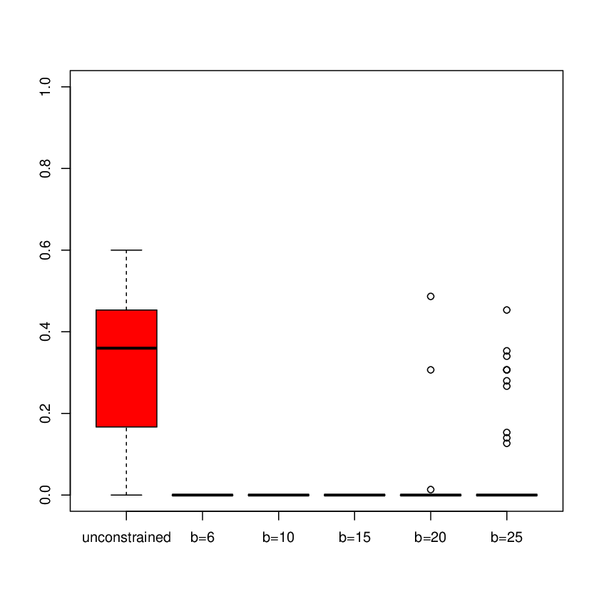
First we run the unconstrained algorithm: the right solution has been attained in 24% of cases, without incurring in singularities. Summary statistics (minimum, first quartile , median , third quartile and maximum) about the distribution of the misclassification error over the 100 runs are reported in Table 2. Due to the choice on parameters, we rarely expect too small eigenvalues in the estimated covariance matrices: we set to protect from them; conversely, as local maxima are quite often due to large estimated eigenvalues, we consider setting also a constraint from above, taking into account some values for , the upper bound. To compare how the choice of the bounds and influences the performance of the constrained EM, we experimented with different pairs of values, and in Table 3 we report the more interesting cases. Further results are reported in Figure 1, which provides the boxplots of the distribution of the misclassification errors obtained in the sequence of runs, showing the poor performance of the unconstrained algorithm compared with the good behaviour of its constrained version. For all values of the upper bound , the third quartile of the misclassification error is steadily equal to . Indeed, for and 15 we had no misclassification error, while we observed very low and rare misclassification errors only for and (respectively 3 and 11 not null values, over 100 runs). Moreover, the robustness of the results with respect to the choice of the upper constraint is apparent.
| Misclassification Error | ||||
| min | max | |||
| 0% | 17% | 36% | 45.3% | 60% |
| 6 | 10 | 15 | 20 | 25 | |
| 24% | 100% | 100% | 100% | 97% | 89% |
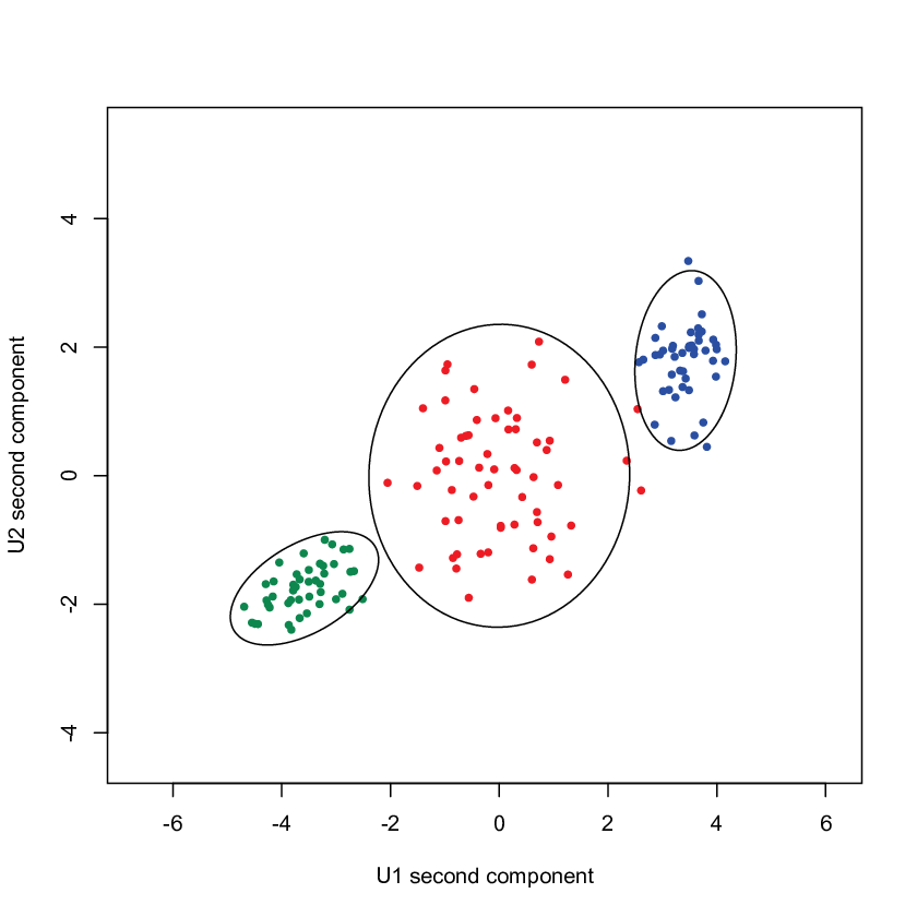
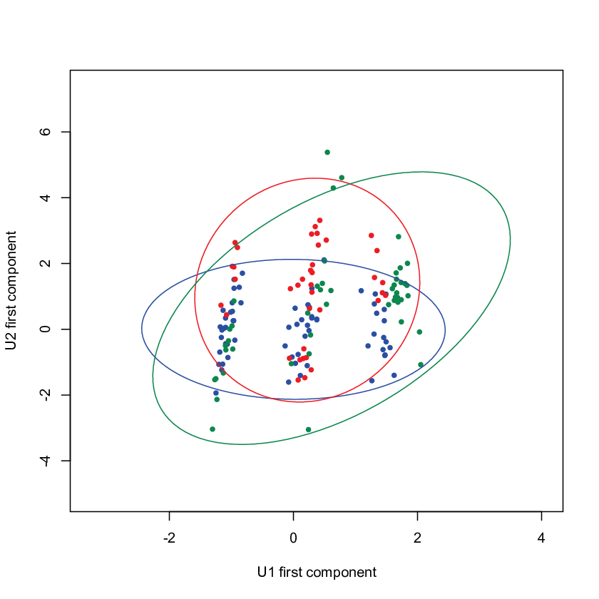
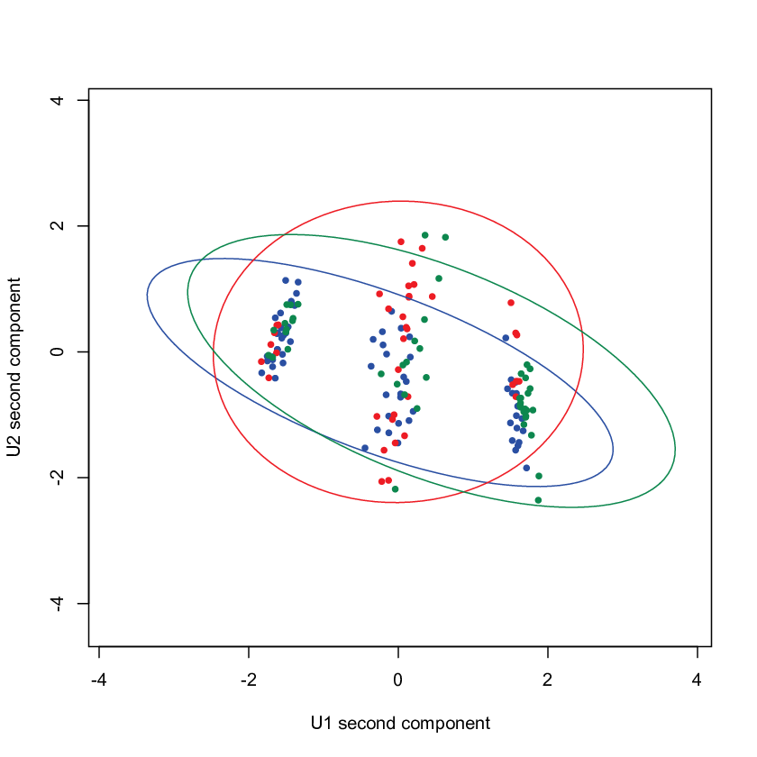
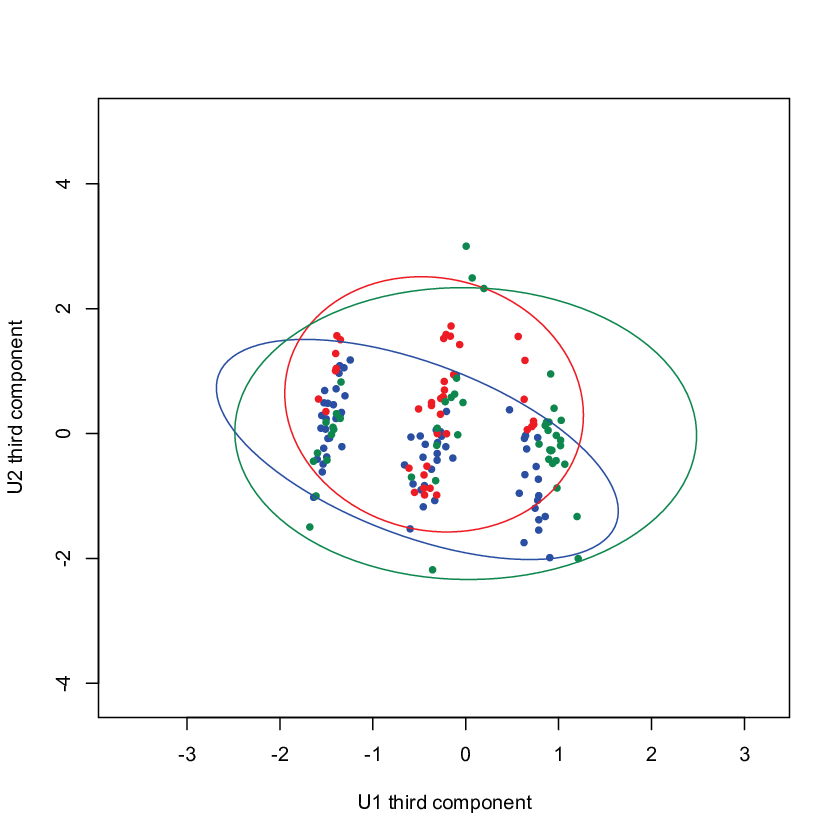
In Figure 2 we plot the classified data on the three factor spaces given by and under the true maximum of the likelihood function (first rows of plots), while in the second row we give the classification obtained according to a spurious maximum of the likelihood function.
We recall that an original data point can be represented in dimensions by the posterior distribution of its associated -dimensional latent factor . A convenient summary of this distribution is its mean. Hence we can portray the in -dimensional space by plotting the estimated conditional expectation of each given , that is, the (estimated) posterior mean of the factor (for ). We have that
where denotes expectation using the estimate instead of , and has been computed following (10).
In the particular case of , as in this simulation experiment, we can draw the data in a bidimensional plot in Figure 2. From the two series of plots, it can be seen that the appropriate factor space allows for the right classification, while a spurious likelihood maximizer leads to unsuitable factor spaces, which in turn generate serious issues in classification.


Mixture 2: , , , .
The sample has been generated with weights according to the following parameters:
The covariance matrices () have respectively the following eigenvalues:
whose largest value is given by
First we run the unconstrained algorithm: the right solution has been attained only once, over 100 runs. Afterwards, we run the constrained algorithm for different values of the upper bound on the largest eigenvalue, while maintaining , and using the same random starting values as before, to compare how the choice of the bounds influences the performance of the constrained EM. In Table 4 we collected the percentage of times in which the algorithm attained the right maximum (where denotes the unconstrained procedure), showing a great improvement with respect to the previous 1% obtained through the unconstrained version.
| 10 | 15 | 20 | 25 | |
| 1% | 69% | 60% | 46% | 33% |
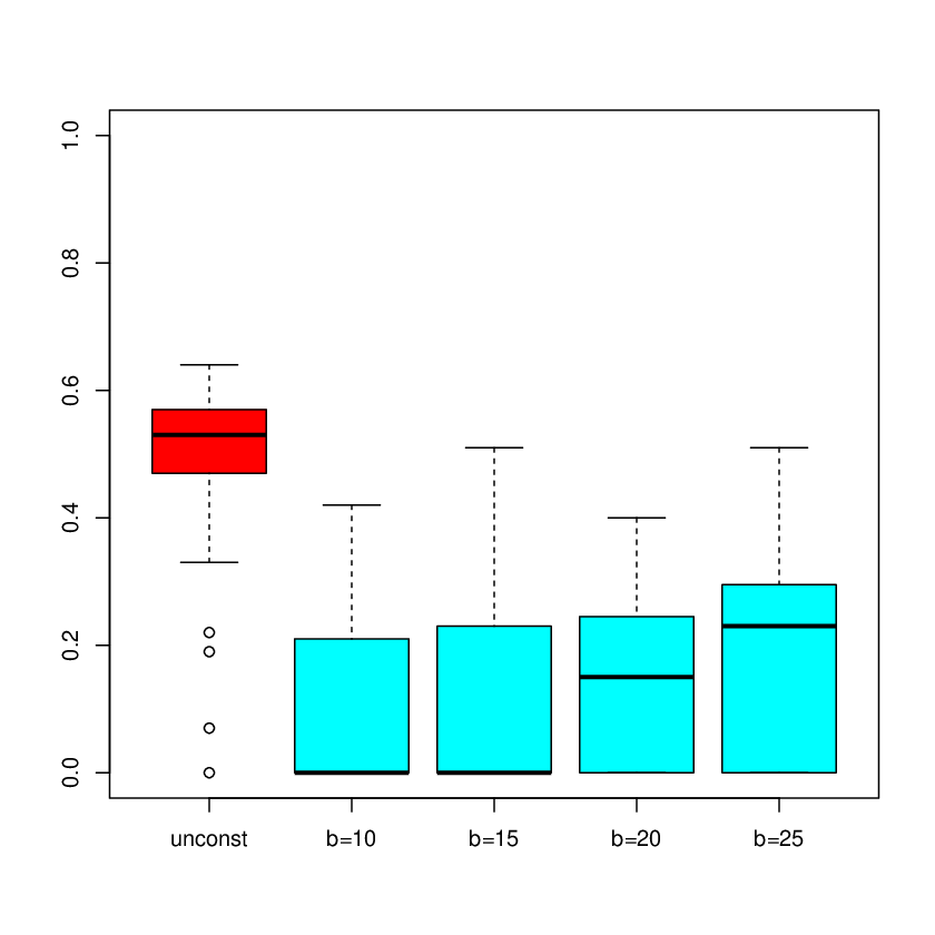
Further details are given in Figure 3 which shows the boxplots of the distribution of the misclassification error in the sequences of runs, corresponding to the different values of the constraint . Also in this case the unconstrained algorithm had a bad performance, with a median misclassification error of 0.53, while its constrained version, for and 15, in more than 50% of the runs had no misclassification error. Furthermore, the unconstrained algorithm did not attain convergence in 4 out of the 100 runs.
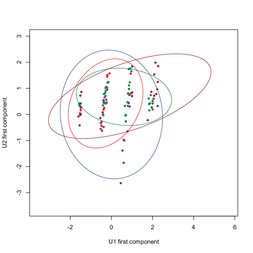
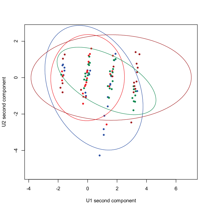
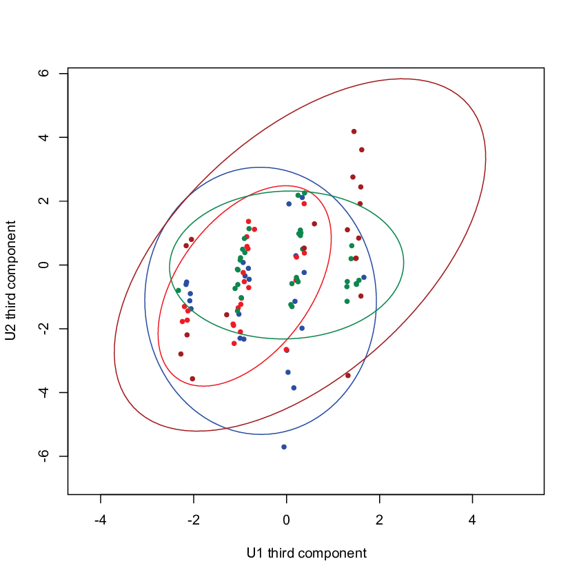
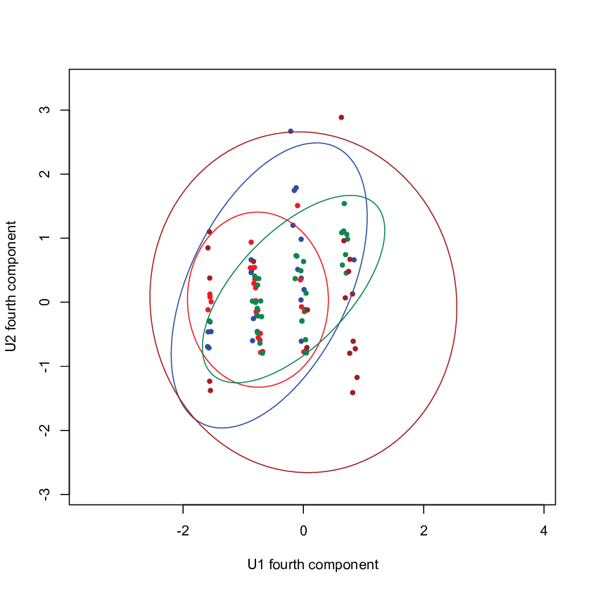
Finally, in Figure 4 we plot the classified data on the factor spaces, under the true maximum of the likelihood function, while in Figure 5 we give the classification in some wrong factor spaces, obtained according to a spurious maximum of the likelihood function.


Mixture 3: , , , .
The third study concerns an artificial dataset analysed in Baek et al. (2010). It has been generated with weights according to the following parameters:
The covariance matrices () have respectively the following eigenvalues:
We run the unconstrained algorithm and its constrained version with the choices of and as before, and also we compare our proposal to the Mixture of Common Factor Analyzers (MCFA) approach of Baek and McLachlan (2011). The percentages of convergence to the right maximum for the seven different cases are reported in Table 5. We recall that MCFA requires a common pattern between covariance matrices. This model is greatly employed in the literature, for parsimony and to avoid potential singularities with small clusters.
| unconstrained | constrained | MCFA | ||||
| 95% | 100% | 96% | 96% | 97% | 97% | 36% |
Over the 100 runs, the MCFA EM algorithm did not converge in 36 cases, while it always reached convergence in the other cases. With respect to the performance of the different algorithms in terms of misclassification error, the corresponding boxplots are shown in Figure 6. We also note that the misclassification error was steadily equal to 1% over the 100 runs for the constrained algorithm with , it was always equal to 1% except 5 runs for the unconstrained algorithm, while in the case of MCFA we have , but and . All these results show that, to attain good performance and robustness in estimation, our proposal works quite better. Furthermore, it allows for a more general solution in comparison to the rigid requirement of a common pattern between covariance matrices. As a consequence, also the log-likelihood of the model obtained by our constrained algorithm () is fairly greater than the log-likelihood obtained in MCFA model ().

6.2 Real data
The Wine data set
Now we consider the wine data, proposed in Forina et al. (1986), consisting of chemical and physical properties of three different cultivars of Italian wine: Barolo, Grignolino and Barbera. This dataset is often used to test and compare the performance of various classification algorithms: among them, in McNicholas and Murphy (2008) using parsimonious Gaussian mixture models and in Andrews and McNicholas (2011) using parsimonious mixtures of multivariate -factor analyzers.
Consider first the complete dataset, with . We run the EM algorithm starting from the true classification, and using the maximum likelihood estimate we get 3 misclassified units (i.e. Misclassification Error ). Based on estimates of and , we get
With the aim at comparing our results with the above findings in the literature, we first scaled the original data, and applied the Pgmm package (McNicholas et al., 2011). Using a set of three random starts, the best model (BIC) for the given range of factors and components (from 1 up to 4) is a CUU model with = 4 and = 3. The CUU acronym stands for a MGFA with patterned covariance matrices, with a common (C) volume and unconstrained (U) shapes and orientations among the =3 components in the mixture. Factors for the best model are of dimension =4, with BIC= -11427.65. The obtained classification is given by Table 6, showing only 2 misclassified units.
| Classification table | |||
|---|---|---|---|
| 1 | 2 | 3 | |
| 1 | 59 | 0 | 0 |
| 2 | 1 | 69 | 1 |
| 3 | 0 | 0 | 48 |
Then we employed our approach, after scaling the data and using hierarchical clustering for initialization (as in the previously cited work). We obtained 5 misclassified units (which means a misclassification error of ). If we initialize the EM algorithm with the true belonging of units and considering still 4-dimensional factors, we obtain a perfect classification. We also obtain a better fit of the model to the data, assessed by a greater penalized likelihood value, namely BIC= -10814.68, due to the lighter constraints we are imposing here. Finally, we employed a mixture of -factor analyzers, applying the teigen R-package (Andrews and McNicholas, 2012), on the scaled data. We considered patterned models, whose label is a sequence of four letters: each letter can be ”C” or ”U” or ”I” denoting ”Constrained to be equal”, ”Unconstrained” and ”Isotropic” patterns on group covariances, and the four letters in the model label are respectively referred to volume, shape, orientation, and the degrees of freedom of the -distribution. We got that the best fit (BIC =-11939.94) is given by CICC model with =5, and this is somehow surprising as we always obtained 3 groups, by all the methods seen so far, in particular also in the proposed constrained EM approach for gaussian factors.
The Flea Beetles data set
The flea beetles data were introduced by Lubischew (1962) and are available within the GGobi software, see Swayne et al. (2006). Data were collected on specimens of flea beetle of the genus Chaetocnema, which contains three species: concinna, heptapotamica, or heikertingeri. Measurements were collected on the width (in the fore-part and from the side) and angle of the aedeagus, on the width of the first and second joint of the tarsus, and on the width of the head between the external edges of the eyes of each beetle.
The goal of the original study was to form a classification rule to distinguish the three species. To this aim, we considered factors, according to the results of Andrews and McNicholas (2011), and we run firstly the unconstrained algorithms. Over the 100 runs, the unconstrained EM algorithm never reached the true solution, and summary statistics (minimum, first quartile , median , third quartile and maximum) about the distribution of the misclassification error over the 100 runs are reported in Table 7.
| Misclassification Error | ||||
| min | max | |||
| 4.1% | 28.0% | 36.5% | 41.9% | 51.4% |
The first results motivated us to run also the constrained EM algorithm, to see if it improves convergence to the right maximum and consequent classification. Tacking into account that
we considered constrained estimation with
lower bound either 0.1 or 0.5, and upper bound either 200 or 300.
Over the 100 runs, the constrained algorithm steadily improves all results, as it can be seen in Table 8, which shows also that the best results can be obtained with the tightest constraints, i.e. .
| unconstrained | constrained | |||
| 0% | 31% | 34% | 21% | 17% |
Figure 7 provides the boxplots of the distribution of the of the misclassification errors in the sequences of runs for both unconstrained and constrained algorithms. The impact of the lower bound on the estimation is critical, but it seems not to depend too much on its value (remember that its purpose is to protect against divergence of the algorithm) while the upper bound crucially drives the classification results, showing the best performance when it mimics the value of the largest eigenvalue of the ’s.

As a final comment, it is worth mentioning that, when dealing with EM estimation based on random starts, authors in the literature usually give results in terms of ”best outcome over a small number of runs”, say 10 runs for instance. Therefore, we can conclude that the constrained algorithm (having a performance of ) provides the true solution and the perfect classification for the Flea Bleetles dataset.
7 Concluding remarks
Mixtures of factor analyzers are commonly used to explain data, in particular, correlation between variables in multivariate observations, allowing also for dimensionality reduction. For these models, as well as for gaussian mixtures, however, the loglikelihood function may present spurious maxima and singularities and this is due to specific patterns of the estimated covariance structure. It is known, from the literature, that a constrained formulation of the EM algorithm considerably reduces such drawbacks for gaussian mixtures. Motivated by these considerations, in this paper we introduced a constrained approach for gaussian mixtures of factor analyzers. In particular we implemented a methodology to maximize the likelihood function in a constrained parameter space, having no singularities and a reduced number of spurious local maxima. The performance of the newly introduced estimation approach has been shown and compared to the usual non-constrained one, as well as to the approach based on common factors. To this purpose we present numerical simulations on synthetic samples and applications to real data sets widely employed in the literature. The results shows that the problematic convergence of the EM, even more critical when dealing with factor analyzers, can be greatly improved.
References
- Aitken (1926) Aitken, A. (1926). On Bernoulli’s numerical solution of algebraic equations. In Proceedings of the Royal Society of Edinburgh, volume 46, pages 289–305.
- Andrews and McNicholas (2011) Andrews, J. and McNicholas, P. (2011). Extending mixtures of multivariate t-factor analyzers. Statistics and Computing, 21(3), 361–373.
- Andrews and McNicholas (2012) Andrews, J. and McNicholas, P. (2012). Model-based clustering, classification, and discriminant analysis with the multivariate t-distribution: The teigen family. Statistics and Computing, 21, 361–373.
- Baek and McLachlan (2011) Baek, J. and McLachlan, G. (2011). Mixtures of common t-factor analyzers for clustering high-dimensional microarray data. Bioinformatics, 27(9), 1269–1276.
- Baek et al. (2010) Baek, J., McLachlan, G., and Flack, L. (2010). Mixtures of factor analyzers with common factor loadings: Applications to the clustering and visualization of high-dimensional data. Pattern Analysis and Machine Intelligence, IEEE Transactions on, 32(7), 1298 –1309.
- Banfield and Raftery (1993) Banfield, J. D. and Raftery, A. E. (1993). Model-based Gaussian and non-Gaussian clustering. Biometrics, 49(3), 803–821.
- Böhning et al. (1994) Böhning, D., Dietz, E., Schaub, R., Schlattmann, P., and Lindsay, B. (1994). The distribution of the likelihood ratio for mixtures of densities from the one-parameter exponential family. Annals of the Institute of Statistical Mathematics, 46(2), 373–388.
- Forina et al. (1986) Forina, M., Armanino, C., Castino, M., and Ubigli, M. (1986). Multivariate data analysis as a discriminating method of the origin of wines. Vitis, 25, 189–201.
- Ghahramani and Hilton (1997) Ghahramani, Z. and Hilton, G. (1997). The EM algorithm for mixture of factor analyzers. Techical Report CRG-TR-96-1.
- Hathaway (1985) Hathaway, R. (1985). A constrained formulation of maximum-likelihood estimation for normal mixture distributions. The Annals of Statistics, 13(2), 795–800.
- Hoff (2005) Hoff, P. (2005). Subset clustering of binary sequences, with an application to genomic abnormality data. Biometrics, 61, 1027–1036.
- Ingrassia (2004) Ingrassia, S. (2004). A likelihood-based constrained algorithm for multivariate normal mixture models. Statistical Methods & Applications, 13, 151–166.
- Ingrassia and Rocci (2007) Ingrassia, S. and Rocci, R. (2007). Constrained monotone em algorithms for finite mixture of multivariate gaussians. Computational Statistics & Data Analysis, 51, 5339–5351.
- Liu et al. (2003) Liu, J., Zhang, J., Palumbo, M., and Lawrence, C. (2003). Bayesian clustering with variable and transformation selection (with discussion). Bayesian Statistics, 7, 249–275.
- Lubischew (1962) Lubischew, A. (1962). On the use of discriminant functions in taxonomy. Biometrics, 18, 455–477.
- Lütkepohl (1996) Lütkepohl, H. (1996). Handbook of matrices. John Wiley & Sons, Chichester.
- McLachlan and Krishnan (2007) McLachlan, G. and Krishnan, T. (2007). The EM algorithm and extensions. John Wiley & Sons, New York.
- McLachlan et al. (2003) McLachlan, G., Peel, D., and Bean, R. (2003). Modelling high-dimensional data by mixtures of factor analyzers. Computational Statistics and Data Analysis, 41, 379–388.
- McLachlan and Peel (2000) McLachlan, G. J. and Peel, D. (2000). Finite Mixture Models. John Wiley & Sons, New York.
- McNicholas and Murphy (2008) McNicholas, P. and Murphy, T. (2008). Parsimonious Gaussian mixture models. Statistics and Computing, 18(3), 285–296.
- McNicholas et al. (2011) McNicholas, P. D., Jampani, K. R., McDaid, A. F., Murphy, T. B., and Banks, L. (2011). pgmm: Parsimonious gaussian mixture models. r package version 1.0.
- Meng and van Dyk (1997) Meng, X. and van Dyk, D. (1997). The EM algorithm – an old folk-song sung to a fast new tune. Journal of the Royal Statistical Society: Series B (Statistical Methodology), 59(3), 511–567.
- Pan and Shen (2007) Pan, W. and Shen, X. (2007). Penalized model-based clustering with application to variable selection). Journal of machine learning research, 8, 1145–1164.
- Peel and McLachlan (2000) Peel, D. and McLachlan, G. (2000). Robust mixture modelling using the distribution. Statistics and Computing, 10(4), 339–348.
- Raftery and Dean (2006) Raftery, A. and Dean, N. (2006). Variable selection for model-based clustering. Journal of the American Statistical Association, 101(473), 168–178.
- Redner and Walker (1984) Redner, R. A. and Walker, H. F. (1984). Mixture densities, maximum likelihood and the em algorithm. SIAM Review, 26(2), pp. 195–239.
- Swayne et al. (2006) Swayne, D., Cook, D., Buja, A., Lang, D., Wickham, H., and Lawrence, M. (2006). Ggobi manual. http://www.ggobi.org/docs/manual.pdf.