Supplementary material

Sparse inverse covariance matrix estimation is a key step in graph learning. To understand the setup, let us consider learning a Gaussian Markov random field (GMRF) of $p$ nodes/variables from a dataset $\mathcal{D}:=\left\{{\bf x}_{1},{\bf x}_{2},\dots,{\bf x}_{m}\right\}$, where ${\bf x}_{j}\in\mathcal{D}$ is a $p$-dimensional random vector, drawn from the Gaussian distribution $\mathcal{N}(\boldsymbol{\mu},\boldsymbol{\Sigma})$. Let ${\bf\Theta}=\boldsymbol{\Sigma}^{-1}$ be the inverse covariance (or the precision) matrix for the model. To satisfy the conditional independencies with respect to the GMRF, ${\bf\Theta}$ must have zero in ${\bf\Theta}_{ij}$ corresponding to the absence of an edge between nodes $i$ and $j$ (Dempster, 1972).

To learn the underlying graph structure from $\boldsymbol{\Sigma}^{-1}$, one can use the empirical covariance matrix $\widehat{\boldsymbol{\Sigma}}$. Unfortunately, this approach is fundamentally ill-posed since the empirical estimates converge to the true covariance at a $(1/\sqrt{m})$-rate (Dempster, 1972). Hence, inferring the true graph structure accurately requires an overwhelming number of samples. Unsurprisingly, we usually have fewer samples than the ambient dimension, compounding the difficulty of estimation.

While the possible GMRF structures are exponentially large, the most interesting graphs are rather simple with a sparse set of edges. Provable learning of such graphs can be achieved by $\ell_{1}$-norm regularization in the maximum log-likelihood estimation:

where $\rho>0$ is a parameter to balance the fidelity error and the sparsity of the solution and $\mathbf{vec}$ is the vectorization operator. Here, $f({\bf\Theta})$ corresponds to the empirical log-likelihood and $g({\bf\Theta})$ is the sparsity-promoting term. Under this setting, the authors in (Ravikumar et al., 2011) prove that $m=\mathcal{O}(d^{2}\log p)$ is sufficient for correctly estimating the GMRF, where $d$ is the graph node-degree. Moreover, the above formulation still makes sense for learning other graph models, such as the Ising model, due to the connection of $f({\bf\Theta})$ to the Bregman distance (Banerjee et al., 2008).

Numerical solution methods for solving problem (1) have been widely studied in the literature. For instance, in (Banerjee et al., 2008; Scheinberg & Rish, 2009; Scheinberg et al., 2010; Hsieh et al., 2011; Rolfs et al., 2012; Olsen et al., 2012) the authors proposed first order primal and dual approaches to (1) and used state-of-the-art structural convex optimization techniques such as coordinate descent methods and Lasso-based procedures. Alternatively, the authors in (Hsieh et al., 2011; Olsen et al., 2012) focused on the second order methods and, practically, achieved fast methods with a high accuracy. In (Scheinberg et al., 2010; Yuan, 2012), the authors studied alternating direction methods to solve (1), while the work in (Li & Toh, 2010) is based on interior point-type methods. Algorithmic approaches where more structure is known a priori can be found in (Lu, 2010).

The complexity of the state-of-the-art approaches mentioned above is dominated by the Cholesky decomposition ($\mathcal{O}(p^{3})$ in general), which currently creates an important scalability bottleneck. This decomposition appears mandatory since all these approaches employ a guess-and-check step-size selection procedures to ensure the iterates remain in the positive definite (PD) cone and the inversion of a $p\times p$ matrix, whose theoretical cost normally scales with the cost of $p\times p$ matrix multiplications ($\mathcal{O}(p^{3})$ direct, $\mathcal{O}(p^{2.807})$ Strassen, and $\mathcal{O}(p^{2.376})$ Coppersmith-Winograd). The inversion operation is seemingly mandatory in the optimization of (1) since the calculation of the descent direction $\nabla f({\bf\Theta}_{i}):=-{\bf\Theta}_{i}^{-1}+\widehat{\boldsymbol{\Sigma}}$ requires it, and quadratic cost approximations to $f({\bf\Theta})$ also need it. Via Cholesky decompositions, one can first check if the current solution satisfies the PD cone constraint and then recycle the decomposition for inversion for the next iteration.

In the context of graph learning, we discuss a specific instance of our framework, which avoids Cholesky decompositions and matrix inversions altogether. Hence, the per iteration complexity of our approach is dominated by the cost of $p\times p$ matrix multiplications. This is because $(i)$ our analytic step-size selection procedure ensures the positive definiteness of the iterates doing away with global strategies such as line-search which demands the objective evaluations (via Cholesky), and $(ii)$ we avoid calculating the gradient explicitly, and hence matrix inversion by a careful dual formulation. As a result, our approach is attractive for distributed and parallel implementations.

Paper outline: In Section 2, we first recall some fundamental concepts of convex optimization and self-concordant functions. Then, we describe the basic optimization set up and show the unique solvability of the problem. In Section 3 we outline our algorithmic framework and describe its analytical complexity. We also deal with the solution of the subproblems by applying the new dual approach in this section. Section 4 presents an application of our theory to graph selection problems. Experimental results on real graph learning problems can be found in Section 5.

Let $h\in\mathcal{C}^{3}(\mathrm{dom}(f))$ be a strictly convex and self-concordant function. For a given vector ${\bf v}\in\mathbb{R}^{n}$, the local norm around ${\bf x}\in\mathrm{dom}(f)$ with respect to $h(\cdot)$ is defined as $\left\|\bf v\right\|_{\bf x}:=\left({\bf v}^{T}\nabla^{2}h({\bf x}){\bf v}\right)^{1/2}$ while the corresponding dual norm is given as $\left\|\bf v\right\|_{\bf x}^{*}:=\left({\bf v}^{T}\nabla^{2}h({\bf x})^{-1}{\bf v}\right)^{1/2}$. Let $\omega:\mathbb{R}\to\mathbb{R}_{+}$ be a function defined as $\omega(t):=t-\ln(1+t)$ and $\omega_{*}:[0,1]\to\mathbb{R}_{+}$ be a function defined as $\omega_{*}(t):=-t-\ln(1-t)$. The functions $\omega$ and $\omega_{*}$ are both nonnegative, strictly convex and increasing. Based on (Nesterov, 2004)[Theorems 4.1.7 & 4.1.8], we recall the following estimates:

where (2) holds for all ${\bf x},{\bf y}\in\mathrm{dom}(f)$, and (3) holds for all ${\bf x},{\bf y}\in\mathrm{dom}(f)$ such that $\left\|{\bf y}-{\bf x}\right\|_{\bf x}<1$.

The proof of this lemma can be done similarly as Theorem 4.1.11, pp. 187 in (Nesterov, 2004). For completeness, we provide it in the supplementary document.

Our algorithmic framework is simply a proximal-Newton method which generates an iterative sequence $\left\{{\bf x}^{k}\right\}_{k\geq 0}$ starting from ${\bf x}^{0}\in\mathrm{dom}(F)$. The new point ${\bf x}^{k+1}$ is computed as ${\bf x}^{k+1}={\bf x}^{k}+\alpha_{k}{\bf d}^{k}$, where $\alpha_{k}\in(0,1]$ is a step size and ${\bf d}^{k}$ is the proximal-Newton-type direction as the solution to the subproblem:

Here, $Q({\bf d};{\bf x}^{k})$ is the following quadratic surrogate of the function $f$ around ${\bf x}^{k}$:

We denote $\mathbf{d}^{k}$ the unique solution of Q ( x k ) . The optimality condition for Q ( x k ) is written as follows:

Lemma 3.1 suggests that we can generate an iterative sequence based on the fixed-point principle. Under certain assumptions, one can ensure that $R_{g}$ is contractive and the sequence generated by this scheme is convergent. Hence, we characterize this below.

In this section, we customize the theory framework of Algorithm 1 by using only Phase 1 to solve the graph selection problem (1).

Overall, Algorithm 2 does not require any matrix inversion operation. It only needs matrix-vector and matrix-matrix calculations, making the parallelization of the code easier. We note that due to the predefined step-size selection $\alpha_{i}$ in Algorithm 1 we do not need to do any backtracking line-search step. This advantage can avoid some overhead computation regarding the evaluation of the objective function which is usually expensive in this application.

For instance, the computation of $\widetilde{\bf Q}_{i}$ and $\boldsymbol{\Delta}_{i}$ require basic matrix multiplications. For the computation of $\lambda_{i}$, we require two trace operations: $\text{tr}({\bf W}_{i})$ in $\mathcal{O}(p)$ time-complexity and $\text{tr}({\bf W}_{i}^{2})$ in $\mathcal{O}(p^{2})$ time-complexity. We note here that, while ${\bf W}_{i}$ is a dense matrix, the trace operation requires only the computation of the diagonal elements of ${\bf W}_{i}^{2}$. Given ${\bf\Theta}_{i}$, $\alpha_{i}$ and $\boldsymbol{\Delta}_{i}$, ${\bf\Theta}_{i+1}$ requires $O(p^{2})$ time-complexity.

To compute (25), we can use the fast projected gradient method (FPGM) (Nesterov, 2007; Beck & Teboulle, 2009) with step size $1/L$ where $L$ is the Lipschitz constant of the gradient of the objective function in (25). It is easy to observe that $L_{i}:=\gamma_{\max}^{2}({\bf\Theta}_{i})$ where $\gamma_{\max}({\bf\Theta}_{i})$ is the largest eigenvalue of ${\bf\Theta}_{i}$. For sparse ${\bf\Theta}_{i}$, we can approximately compute $\gamma_{\max}({\bf\Theta}_{i})$ is $\mathcal{O}(p^{2})$ by using iterative power methods (typically, 10 iterations suffice). The projection onto $\left\|\text{{vec}}({\bf U})\right\|_{\infty}\leq 1$ clips the elements by unity in $\mathcal{O}(p^{2})$ time. Thus, the time overhead due to acceleration is within $\mathcal{O}(p^{2})$.

Given the above, FPGM requires a constant number of iterations $k_{\max}$, which is independent of the dimension $p$, to achieve an $\varepsilon_{\mathrm{in}}$ solution accuracy. Overall, the time-complexity for the solution in (25) is $\mathcal{O}(k_{\max}M)$, where $M$ is the cost of matrix multiplication.

In this section we test DPNGS (Algorithm 2 in Section 4) and compare it with the state-of-the-art graph selection algorithm QUadratic Inverse Covariance (QUIC) algorithm (Hsieh et al., 2011) on a real world data set. The QUIC algorithm is also a Newton-based method, which in addition exploits the sparsity in solving its primal subproblems. We note that QUIC was implemented in C while our codes in this work are implemented in MATLAB.

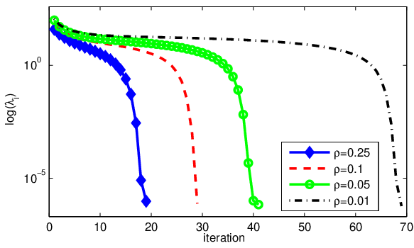
Figure 1 shows that whenever the values of $\lambda_{i}$ gets into the quadratic region, it converges with only a few iterations. As $\rho$ becomes smaller, we need more iterations to get into the quadratic convergence region.

Next, we illustrate the step-size $\alpha_{i}$ of DPNGS. Figure 2 shows the increasing behaviour of the step size on the same dataset. Since $\alpha_{i}=(1+\lambda_{i})^{-1}$, it converges quickly at the last iterations.

We also compare the objective value decrement of both algorithms in $y$-log-scale in Figure 3. Using the same tolerance level, we reach the objective value $-4.141662\times 10^{2}$ after $69$ iterations while QUIC needs $159$ iterations. Moreover, Figure 3 shows the quadratic convergence of our approach in contrast to QUIC; the latter requires many more iterations to slightly improve the objective.

Figure 4 is the histogram of the solution in $\log$ scale reported by DPNGS and QUIC. Due to the dual solution approach, DPNGS reports an approximate solution with similar sparsity pattern as the one of QUIC. However, our solution has many small numbers instead of zero as in QUIC as revealed in Figure 4. This seems to be the main weakness of the dual approach: it obviates matrix inversions by avoiding the primal problem, which can return solutions with exact zeros thanks to its soft-thresholding prox-operator.

As a result, DPNGS carries around extremely small coefficients (almost of them smaller than $5\times 10^{-5}$) often preventing it from achieving the same objective level as the numerical experiments on the full data set shows. At the same time, since the approach does not rely on coordinate descent on active sets, it appears much less sensitive to the choice of $\rho$. This could be an advantage of DPNGS in applications requiring smaller $\rho$ values. If exact sparsity is needed, then a single primal iteration suffices to remove the small coefficients.

We highlight several interesting results from Table 1. First, QUIC obtains the highest accuracy results in most cases, which we attribute to the “lack of soft thresholding” in our algorithm. As the DPNGS algorithm carries around a score of extremely small numbers (effectively making the solution dense in the numerical sense), its solutions are close to QUIC’s solutions within numerical precision. Moreover, QUIC is extremely efficient when the $\rho$ value is large, since it exploits the sparsity of the putative solutions via coordinate descent. Unsurprisingly, QUIC slows down significantly as $\rho$ is decreased.

DPGNS(5) and DPNGS(10) can obtain near optimal solutions quite rapidly. In particular, DPNGS(10) seems to be the most competitive across the board, often taking a fraction of QUIC’s time to provide a very close solution. Hence, one can expect these schemes to be used for initializing other algorithms. For instance, QUIC can be a good candidate. We observed in all cases that, in the first few iterations, QUIC performs several Cholesky decompositions to stay within the positive definite cone. As the complexity of such operation is large, our step-size selection within QUIC or a DPNGS(10) initialization can be helpful.

In this paper, we present the new composite self-concordant optimization framework. As a concrete application, we demonstrate that graph learning is possible without any Cholesky decompositions via analytic step-size selection as well as without matrix inversions via a careful dual formulation within our framework. By exploiting the self-concordance in the composite graph learning objective, we provide an optimal step-size for this class of composite minimization with proximal Newton methods. We show that within the dual formulation of the Newton subproblem, we do not need to explicitly calculate the gradient as it appears in a multiplication form with the Hessian. Thanks to the special structure of this multiplication, we avoid matrix inversions in graph learning. Overall, we expect our optimization framework to have more applications in signal processing/machine learning and be amenable to various parallelization techniques, beyond the ones considered in the graph learning problem.

References

- Banerjee et al. (2008) Banerjee, O., El Ghaoui, L., and d’Aspremont, A. Model selection through sparse maximum likelihood estimation for multivariate gaussian or binary data. The Journal of Machine Learning Research, 9:485–516, 2008.
- Beck & Teboulle (2009) Beck, A. and Teboulle, M. A Fast Iterative Shrinkage-Thresholding Algorithm for Linear Inverse Problems. SIAM J. Imaging Sciences, 2(1):183–202, 2009.
- Bertsekas & Tsitsiklis (1989) Bertsekas, D.P. and Tsitsiklis, J. N. Parallel and distributed computation: Numerical methods. Prentice Hall, 1989.
- Boyd & Vandenberghe (2004) Boyd, S. and Vandenberghe, L. Convex Optimization. University Press, Cambridge, 2004.
- Dempster (1972) Dempster, A. P. Covariance selection. Biometrics, 28:157–175, 1972.
- Hsieh et al. (2011) Hsieh, C. J., Sustik, M.A., Dhillon, I.S., and Ravikumar, P. Sparse inverse covariance matrix estimation using quadratic approximation. Advances in Neutral Information Processing Systems (NIPS), 24:1–18, 2011.
- Lee et al. (2012) Lee, J.D., Sun, Y., and Saunders, M.A. Proximal newton-type methods for convex optimization. Tech. Report., pp. 1–25, 2012.
- Li & Toh (2010) Li, L. and Toh, K.C. An inexact interior point method for l 1-regularized sparse covariance selection. Mathematical Programming Computation, 2(3):291–315, 2010.
- Lu (2010) Lu, Z. Adaptive first-order methods for general sparse inverse covariance selection. SIAM Journal on Matrix Analysis and Applications, 31(4):2000–2016, 2010.
- Nesterov (2004) Nesterov, Y. Introductory lectures on convex optimization: a basic course, volume 87 of Applied Optimization. Kluwer Academic Publishers, 2004.
- Nesterov (2007) Nesterov, Y. Gradient methods for minimizing composite objective function. CORE Discussion paper, 76, 2007.
- Nesterov & Nemirovski (1994) Nesterov, Y. and Nemirovski, A. Interior-point Polynomial Algorithms in Convex Programming. Society for Industrial Mathematics, 1994.
- Olsen et al. (2012) Olsen, P.A., Oztoprak, F., Nocedal, J., and Rennie, S.J. Newton-like methods for sparse inverse covariance estimation. Optimization Online, 2012.
- Ravikumar et al. (2011) Ravikumar, P., Wainwright, M. J., Raskutti, G., and Yu, B. High-dimensional covariance estimation by minimizing l1-penalized log-determinant divergence. Electron. J. Statist., 5:935–988, 2011.
- Rolfs et al. (2012) Rolfs, B., Rajaratnam, B., Guillot, D., Wong, I., and Maleki, A. Iterative thresholding algorithm for sparse inverse covariance estimation. In Advances in Neural Information Processing Systems 25, pp. 1583–1591, 2012.
- Scheinberg & Rish (2009) Scheinberg, K. and Rish, I. Sinco-a greedy coordinate ascent method for sparse inverse covariance selection problem. preprint, 2009.
- Scheinberg et al. (2010) Scheinberg, K., Ma, S., and Goldfarb, D. Sparse inverse covariance selection via alternating linearization methods. arXiv preprint arXiv:1011.0097, 2010.
- Yuan (2012) Yuan, X. Alternating direction method for covariance selection models. Journal of Scientific Computing, 51(2):261–273, 2012.
Appendix A The proofs of technical statements
A.1 The proof of Theorem 3.2
Proof.
Let , we define
and
It follows from the optimality condition (7) in the main text that
This condition can be written equivalently to
Therefore, the last relation leads to