GESPAR: Efficient Phase Retrieval of
Sparse Signals
Abstract
We consider the problem of phase retrieval, namely, recovery of a signal from the magnitude of its Fourier transform, or of any other linear transform. Due to the loss of the Fourier phase information, this problem is ill-posed. Therefore, prior information on the signal is needed in order to enable its recovery. In this work we consider the case in which the signal is known to be sparse, i.e., it consists of a small number of nonzero elements in an appropriate basis. We propose a fast local search method for recovering a sparse signal from measurements of its Fourier transform (or other linear transform) magnitude which we refer to as GESPAR: GrEedy Sparse PhAse Retrieval. Our algorithm does not require matrix lifting, unlike previous approaches, and therefore is potentially suitable for large scale problems such as images. Simulation results indicate that GESPAR is fast and more accurate than existing techniques in a variety of settings.
I Introduction
Recovery of a signal from the magnitude of its Fourier transform, also known as phase retrieval, is of great interest in applications such as optical imaging [1], crystallography [2], and more [3]. Due to the loss of Fourier phase information, the problem (in 1D) is generally ill-posed. A common approach to overcome this ill-posedeness is to exploit prior information on the signal. A variety of methods have been developed that use such prior information, which may be the signal’s support (region in which the signal is nonzero), non-negativity, or the signal’s magnitude [4], [5].
A popular class of algorithms is based on the use of alternate projections between the different constraints. In order to increase the probability of correct recovery, these methods require the prior information to be very precise, for example, exact/or “almost” exact knowledge of the support set. Since the projections are generally onto non-convex sets, convergence to a correct recovery is not guaranteed [6]. A more recent approach is to use matrix-lifting of the problem which allows to recast phase retrieval as a semi-definite programming (SDP) problem [7]. The algorithm developed in [7] does not require prior information about the signal but instead uses multiple signal measurements (e.g., using different illumination settings, in an optical setup).
In order to obtain more robust recovery without requiring multiple measurements, we develop a method that exploits signal sparsity. Existing approaches aimed at recovering sparse signals from their Fourier magnitude belong to two main categories: SDP-based techniques [8],[9],[10],[11] and algorithms that use alternate projections (Fienup-type methods) [12]. Phase retrieval of sparse signals can be viewed as a special case of the more general quadratic compressed sensing (QCS) problem considered in [8]. Specifically, QCS treats recovery of sparse vectors from quadratic measurements of the form , where is the unknown sparse vector to be recovered, are the measurements, and are known matrices. In (discrete) phase retrieval, where is the th row of the discrete Fourier transform (DFT) matrix. QCS is encountered, for example, when imaging a sparse object using partially spatially-incoherent illumination [8].
A general approach to QCS was developed in [8] based on matrix lifting. More specifically, the quadratic constraints where lifted to a higher dimension by defining a matrix variable . The problem was then recast as an SDP involving minimization of the rank of the lifted matrix subject to the recovery constraints as well as row sparsity constraints on . An iterative thresholding algorithm based on a sequence of SDPs was then proposed to recover a sparse solution. Similar SDP-type ideas were recently used in the context of phase retrieval [9],[10]. However, due to the increase in dimension created by the matrix lifting procedure, the SDP approach is not suitable for large-scale problems.
Another approach for phase retrieval of sparse signals is adding a sparsity constraint to the well-known iterative error reduction algorithm of Fienup [12]. In general, Fienup-type approaches are known to suffer from convergence issues and often do not lead to correct recovery especially in 1D problems; simulation results show that even with the additional information that the input is sparse, convergence is still problematic and the algorithm often recovers erroneous solutions.
In this paper we propose an efficient method for phase retrieval which also leads to good recovery performance. Our approach is based on a fast 2-opt local search method (see [13] for an excellent introduction to such techniques) applied to a sparsity constrained non-linear optimization formulation of the problem. We refer to the resulting algorithm as GESPAR: GrEedy Sparse PhAse Retrieval. Sparsity constrained nonlinear optimization problems have been considered recently in [14]; the method derived in this paper is motivated – although different in many aspects – by the local search-type techniques of [14]. In essence, GESPAR is a local-search method, where the support of the sought signal is updated iteratively, according to selection rules described in detail in Section III. A local minimum of the objective function is then found given the current support using the damped Gauss Newton algorithm. Theorem 1 establishes convergence of the iterations to a stationary point of the objective under suitable conditions.
We demonstrate through numerical simulations that GESPAR is both efficient and more accurate than current techniques. Several other aspects of the algorithm are explored via simulations such as robustness to noise, and scalability for larger dimensions. In the simulations performed we found that the number of measurements needed for reliable recovery from Fourier magnitudes seems to scale like , where is the sparsity level.
GESPAR is applicable to recovery of a sparse vector from general quadratic measurements, and is not restricted to Fourier magnitude measurements. Nonetheless, when the measurements are obtained in the Fourier domain, the algorithm can be implemented efficiently by exploiting the fast Fourier transform, as we discuss in Section IV.
The remainder of the paper is organized as follows. We formulate the problem in Section II. Section III describes our proposed algorithm in detail and establishes convergence of the local iterations. Implementation details for Fourier-based problems are provided in Section IV. Extensive numerical experiments illustrating the empirical performance of GESPAR are presented in Section V.
II Problem Formulation
II-A Sparse Phase Retrieval: Fourier Measurements
We are given a vector of measurements , that corresponds to the magnitude-squared of an point DFT of a vector , i.e.:
| (1) |
Here is constructed by zero padding of a vector with elements . Denoting by the DFT matrix with elements , we can express as , where denotes the element-wise absolute-squared value. The vector is known to be -sparse, that is, it contains at most nonzero elements. Our goal is to recover , or , given the measurements and the sparsity level .
The mathematical formulation of the problem that we consider consists of minimizing the sum of squared errors subject to the sparsity constraint:
| (2) |
where is the th row of the DFT matrix , and stands for the zero-“norm”, that is, the number of nonzero elements. Note that the unknown vector can only be found up to trivial degeneracies that are the result of the loss of Fourier phase information: circular shift, global phase, and signal “mirroring”.
Support Information
To aid in solving the phase retrieval problem, we can rely on the fact that the autocorrelation sequence of (the first components of ) may be determined from if . Specifically, let
| (3) |
denote the correlation sequence of length . If we choose , then can be obtained by taking the inverse DFT of .
Determining requires oversampling, or zero-padding of . While this additional information improves the recovery performance, as is demonstrated in the simulations section, it is not actually needed for GESPAR to work. Nevertheless, when this information is available, GESPAR exploits it, in the following way. First of all, we assume that no support cancelations occur in , namely, if and for some , then . When the values of are random, this is true with probability 1. This fact can be used in GESPAR in order to obtain initial information on the support of , which we capture by two sets and .
Denote by the set of indices known in advance to be in the support. To derive the set , note that due to the existing degree of freedom relating to shift-invariance of , the index 1 can be assumed to be in the support, thereby removing this degree of freedom; as a consequence, the index corresponding to the last nonzero element in the autocorrelation sequence is also in the support, i.e.
Therefore,
Next, we denote by the set of indices that are candidates for being in the support, meaning the indices that are not known in advance to be in the off-support (the complement of the support). Specifically, contains the set of all indices such that . Obviously, since we assume that for , we have . As a concrete example, consider the signal . The corresponding point autocorrelation function is given by . The set is therefore . Next, by examining the zeros of , and using our assumption of no support-cancelations, we deduce that there are no two non-zero elements and such that . Therefore, forcing the first element in to be non-zero, which removes the shift-invariance degeneracy, immediately implies that In this way is determined as Defining , problem (2) along with the support information can be written as
| (4) |
which will be the formulation to be studied.
Note that even with knowledge of the exact support of there is no guarantee for uniqueness beyond the aforementioned trivial degeneracies. Consider for example the two vectors and . Both of these vectors are sparse, and they have the same autocorrelation function . This ambiguity therefore cannot be resolved using any method that uses sparsity (even exact support information) and autocorrelation (or Fourier magnitude) measurements alone.
Finally, when the measurements are noisy, the autocorrelation information is not very useful for support estimation, since very small (noise level) values in the autocorrelation sequence cannot be treated as zero. For this reason, the autocorrelation-derived support information is not used in GESPAR at all in the noisy case. Formally, ignoring this information is equivalent to setting and .
II-B Sparse Phase Retrieval: General Measurements
Although the problem formulation above assumes Fourier measurements and sparsity of , we show below that our approach applies to arbitrary quadratic measurements of . This includes the case in which is sparse in a basis other than the identity basis. In fact, in this general case, the formulation given in (4) remains the same, with the only change being the definition of the matrices .
Consider the phase retrieval problem with respect to arbitrary linear measurements, so that
| (5) |
for a set of measurement vectors . The corresponding phase retrieval problem can be written as in (4) with . Similarly, suppose that , where is some basis in which is sparse, and is a sparse vector. In this case . Thus, our formulation can accommodate arbitrary sparsity bases and general quadratic measurements.
In the next section, we propose GESPAR—an iterative local-search based algorithm for solving (4). We note that although in the context of phase retrieval the parameters have special properties (e.g., is positive semidefinite of at most rank 2, ), we will not use these properties in GESPAR. Therefore, our approach is capable of handling general instances of (4) with the sole assumption that is symmetric for any . In the Fourier case, the algorithm can be implemented more efficiently, as we discuss in Section IV.
III GrEedy Sparse PhAse Retrieval (GESPAR)
III-A The Damped Gauss-Newton Method
Before describing our algorithm, we begin by presenting a variant of the damped Gauss-Newton (DGN) method [15],[16] that is in fact the core step of our approach. The DGN method is invoked in order to solve the problem of minimizing the objective function over a given support :
| (6) |
where is the matrix consisting of the columns of the identity matrix corresponding to the index set . With this notation, (6) can be explicitly written as
| (7) |
The minimization in (7) is a nonlinear least-squares problem. A natural approach for tackling it is via the DGN method. This algorithm begins with an arbitrary vector . In our simulations, we choose it as a white random Gaussian vector with zero mean and unit variance. At each iteration, all the terms inside the squares in are linearized around the previous guess. Namely, we write from (7) as:
| (8) |
with , and . At each step we replace by its linear approximation around :
| (9) | |||||
We then choose to be the solution of the problem
| (10) |
Problem (10) can be written as a linear least-squares problem
| (11) |
with the th row of being , and the th component of given by for . The solution is equal to . We then define a direction vector . This direction is used to update the solution with an appropriate stepsize designed to guarantee the convergence of the method to a stationary point of . The stepsize is chosen via a simple backtracking procedure. Algorithm 1 describes the DGN method in detail. In our implementation the stopping parameters were chosen as and .
The following theorem establishes the rate of convergence of the norm of the gradient of the objective function to zero, and consequently proves that the limit points of the sequence are stationary points.
Theorem 1.
Let be the sequence generated by the DGN method. Assume that and that there exists such that for all
Then as and there exists a constant such that
| (12) |
Moreover, each limit point of the sequence is a stationary point of .
Proof.
See Appendix A. ∎
Note that the proof requires to have full column rank, and in fact that the minimum eigenvalues of are uniformly bounded below. In the vast majority of our runs this assumption held true; however, we did encounter in our numerical experiments a few cases in which this condition was not valid. In these situations, our implementation chose one of the optimal solutions of the corresponding least-squares problem. We noticed that these cases had negligible effect on the results.
Input: .
- symmetric matrices.
- index set.
- stopping criteria parameter.
- maximum allowed iterations.
Output: - an optimal (or suboptimal) solution of (7).
Initialization: Set ,
a random vector.
General Step : Given the iterate , the next iterate is determined as follows:
1. Gauss-Newton Direction: Let be the solution of the linear least-squares problem (11), given by:
with the th row of being , and the th component of given by . The Gauss-Newton direction is
2. Stepsize Selection via Backtracking: set . Choose a stepsize as , where is the minimal nonnegative integer for which
with given by (7).
3. Update: set
4. Stopping rule: STOP if either
or .
III-B The 2-opt Local Search Method
The GESPAR method consists of repeatedly invoking a local-search method on an initial random support set. In this section we describe the local search procedure. At the beginning, the support is chosen to be a set of random indices chosen to satisfy the support constraints . Then, at each iteration a swap between a support and an off-support index is performed such that the resulting solution via the DGN method improves the objective function. Since at each iteration only two elements are changed (one in the support and one in the off-support), this is a so-called “2-opt” method (see [13]). The swaps are always chosen to be between the index corresponding to components in the current iterate with the smallest absolute value and the off-support index corresponding to the component of with the largest absolute value. This process continues as long as the objective function decreases and stops when no improvement can be made. A detailed description of the method is given in Algorithm 2.
Input: ().
- symmetric matrices.
Output: - a suggested solution for problem (4).
- total number of required swaps.
- 1.
Initialization:
- (a)
Set .
- (b)
Generate a random index set satisfying the support constraints ().
- (c)
Invoke the DGN method with parameters and obtain an output . Set .
- (a)
- 2.
General Step ():
- (a)
Let be the index from corresponding to the component of with the smallest absolute value. Let be the index from corresponding to the component of with the highest absolute value.
- (b)
Set , and make a swap between the indices and
Invoke DGN with input and obtain an output . Set . Advance : .
If , then set , advance and goto 2.a. - (c)
If none of the swaps resulted with a better objective function value, then STOP. The output is and .
- (a)
III-C The GESPAR Algorithm
The 2-opt method can have the tendency to get stuck at local optima points. Therefore, our final algorithm, which we call GESPAR, is a restarted version of 2-opt. The 2-opt method is repeatedly invoked with different initial random support sets until the resulting objective function value is smaller than a certain threshold (success) or the number of maximum allowed total number of swaps was passed (failure). A detailed description of the method is given in Algorithm 3. One element of our specific implementation that is not described in Algorithm 3 is the incorporation of random weights added to the objective function, giving randomly different weights to the different measurements. Namely, the objective function used is actually chosen as with or with equal probability. The random generation of weights is done each time the DGN procedure is invoked. We observed that this modification reduced the probability of the 2-opt procedure to get stuck in non-optimal points.
Input: ().
- symmetric matrices.
- threshold parameter.
ITER - Maximum allowed total number of swaps.
Output: - an optimal (or suboptimal) solution of (4).
Initialization. Set .
- •
Repeat
Invoke the 2-opt method with input () and obtain an output and . Set and advance : .
Until or . - •
The output is where .
IV Fourier Implementation Details
In principle, GESPAR may be used to find sparse solutions to any system of quadratic equations, i.e. problems of the form:
| (13) |
However, when the matrices correspond to transforms that can be implemented efficiently, GESPAR takes on a particularly simple form.
For example, consider the case in which represent Fourier measurements. In this case, the creation and storing of the matrices defined in Section II, can be avoided in the implementation, by using the FFT. Specifically, to calculate the weighted objective function, we note that
| (14) |
where is the th DFT component of , which can be computed via the FFT. Clearly, , which is used in the DGN procedure (Algorithm 1) can also be computed efficiently since only involves a small () number of columns of the Fourier matrix .
The FFT can also be used in the calculation of the gradient , used in the 2-opt stage 2:
| (15) |
Consequently, in no step of the algorithm is it necessary to calculate the set of matrices explicitly.
This fact is even more important in the 2D Fourier phase retrieval problem, as the relevant vector sizes become very large. Since a major advantage of GESPAR over other methods (e.g. SDP based) is its low computational cost, GESPAR may be used to find a sparse solution to the 2D Fourier phase retrieval - or phase retrieval of images. The only adjustments needed in the algorithm are in the implementation, for example, using FFT2 instead of storing the large matrices .
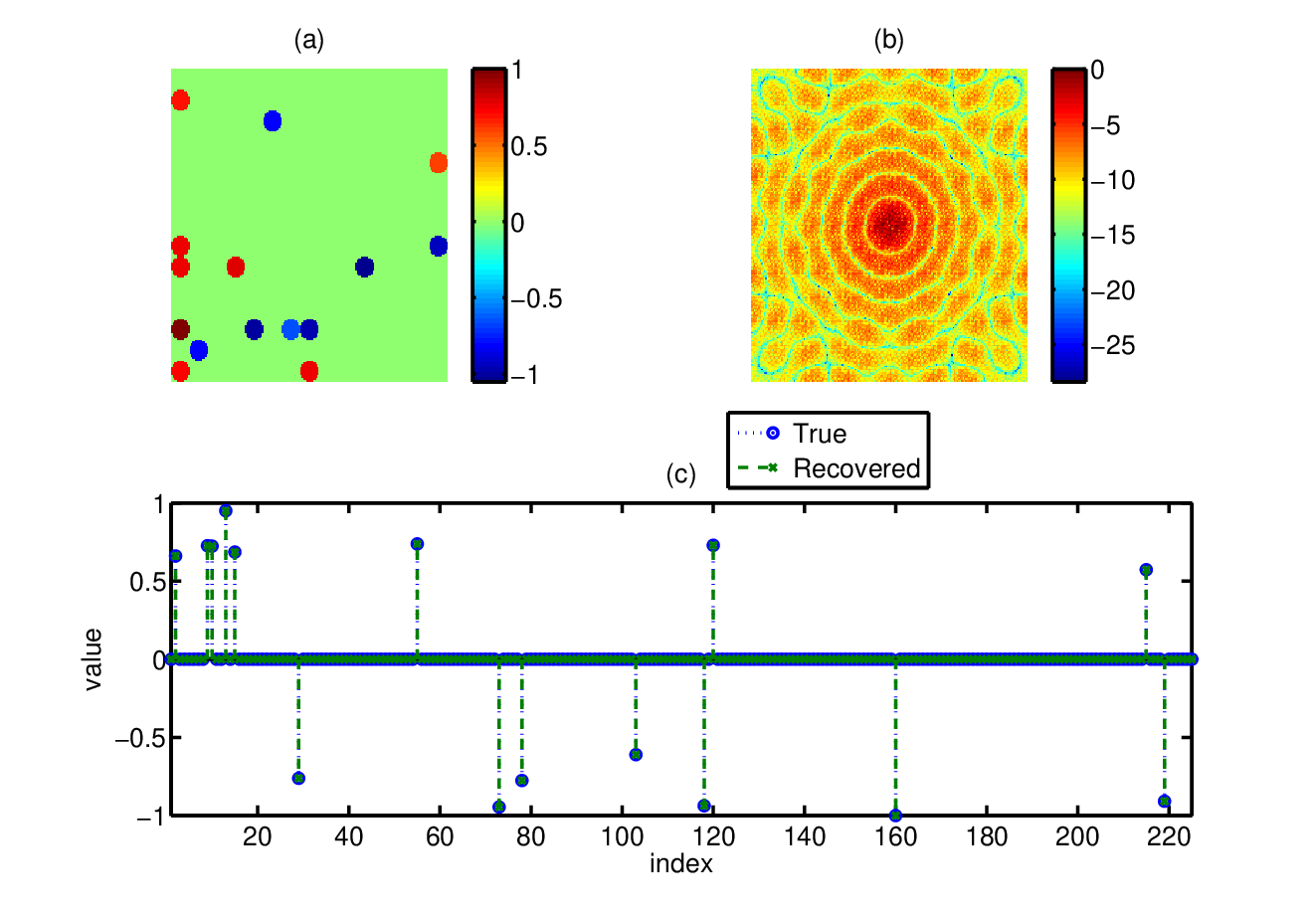
Figure 1 shows a recovery example of a sparse pixel image, comprised of circles at random locations and random values on a grid containing points, recovered from its 2D-Fourier magnitude measurements, using GESPAR. The dictionary used in this example contains 225 elements consisting of non-overlapping circles located on a point cartesian grid, each with a 13 pixel diameter. The solution took 80 seconds. Solving the same problem using the sparse Fienup algorithm did not yield a successful reconstruction, and using the SDP method is not practical due to the large matrix sizes.
Further investigation of the algorithm’s performance in the 2D case is presented in Section V.
V Numerical Simulations
In order to demonstrate the performance of GESPAR, we conduct several numerical simulations. The algorithm is compared to other existing methods, and is evaluated in terms of signal-recovery accuracy, computational efficiency, and robustness to noise.
V-A Signal-recovery Accuracy
In this subsection we examine the recovery success rate of GESPAR as a function of the number of non-zero elements in the signal. A runtime comparison of the tested methods is also performed.
We choose as a random vector of length . The vector contains uniformly distributed values in the range in randomly chosen elements. The point DFT of the signal is calculated, and its magnitude-square is taken as , the vector of measurements. The point correlation is also calculated. In order to recover the unknown vector , the GESPAR algorithm is used with and . We also test two other algorithms for comparison purposes: An SDP based algorithm (Algorithm 2, [9]), and an iterative Fienup algorithm with a sparsity constraint [12]. In our simulation and . The Sparse-Fienup algorithm is run using random initial points, out of which the chosen solution is the one that best matches the measurements. Namely, is selected as the sparse output of the Sparse-Fienup algorithm with the minimal cost out of the runs.
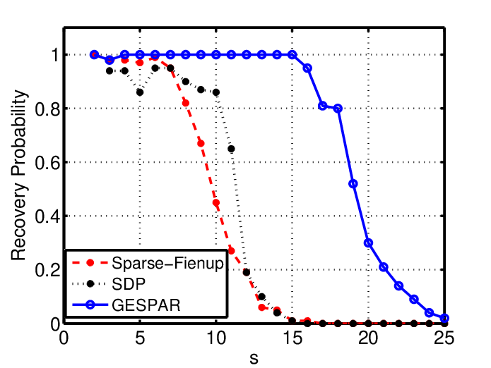
Signal recovery results of the numerical simulation are shown in Fig. 2, where the probability of successful recovery is plotted for different sparsity levels. The success probability is defined as the ratio of correctly recovered signals out of simulations. In each simulation both the support and the signal values are randomly selected. The three algorithms (GESPAR, SDP and Sparse-Fienup) are compared. The results clearly show that GESPAR outperforms the other methods in terms of probability of successful recovery - over 90% successful recovery up to , vs. and in the other two techniques.
Average runtime comparison of the three algorithms is shown in Table I for and . The runtime is averaged over all successful recoveries. The computer used has an intel i5 CPU and 4GB of RAM. As seen in the table, the SDP based algorithm is significantly slower than the other two methods. Fienup iterations are slightly slower than GESPAR and lead to a much lower success rate. In these simulations, GESPAR is both fast and more accurate than its competitors.
| SDP | Sparse-Fienup | GESPAR | ||||
| recovery % | runtime sec | recovery % | runtime sec | recovery % | runtime sec | |
| 0.93 | 1.32 | 0.98 | 0.09 | 1 | 0.04 | |
| 0.86 | 1.78 | 0.97 | 0.12 | 1 | 0.05 | |
| 0.9 | 3.85 | 0.82 | 0.50 | 1 | 0.06 | |
V-B Sensitivity to exact sparsity knowledge
Since the exact value of the signal’s sparsity may not be known, the performance of GESPAR is examined when only an upper limit on is given. To this end we run GESPAR twice: Once with known exactly at each realization, and once with only an upper limit on . The upper limit is taken as . The other simulation settings are the same as in SectionV-A.
Figure 3 shows the probability for successful recovery of the two simulations. The rather loose upper limit on does not seem to affect the results significantly— in fact, the performance is somewhat improved when allowing more nonzero elements during the iterations.

V-C Effect of the number of allowed swaps
One of the stopping criteria for the GESPAR algorithm is when the total number of swaps exceeds a predefined parameter (the input parameter in Algorithm 3). Naturally, increasing the allowed number of index swaps will increase the probability of finding a correct solution, but at the cost of increased computation time. It is therefore important to quantify this effect, which is the purpose of the current simulation.
We run GESPAR with the same parameters as in SectionV-A several times, where in each simulation a different value for the parameter is used, in the range . Figure 4 shows the results. As expected, increasing the number of possible swaps increases the recovery probability. Note that increasing the value of above demonstrated no improvement in the recovery results - for the unsuccessful recoveries, increasing the number of swaps even up to did not help. This means that for these simulation values (e.g. ), using a value of larger than only increases computation time without improving the results.

V-D Effect of oversampling and support information
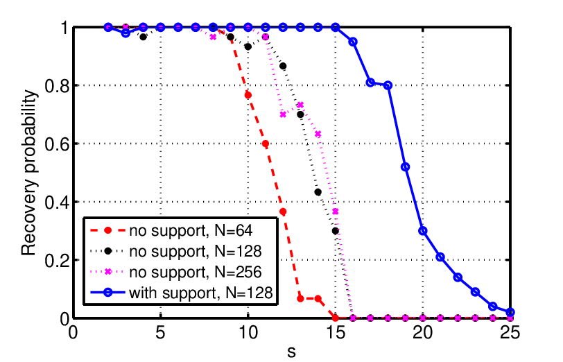
Here we examine the effect of oversampling and of autocorrelation-derived support information. GESPAR is run on random vectors of length , with a varying amount of noiseless Fourier magnitude measurements, obtained by the point DFT of with . In these cases, no support information was used - i.e. and . In addition, in order to investigate the effect of support information, we run GESPAR with (i.e. oversampling by a factor of 2), and use the support information derived from the autocorrelation sequence. The results, shown in Fig. 5, clearly show that both oversampling and support information improve performance.
V-E Robustness to noise
We now evaluate GESPAR as a function of SNR, and compare it with sparse Fienup [12]. The SDP based method presented in [9] is not designed to deal with noise and therefore we did not apply it here. The SDP approach of [10] considers random measurements, and does not produce comparable results from direct Fourier measurements.
As in Section V-A, we choose as a vector of length , with randomly chosen elements containing uniformly distributed values, and evaluate its point Fourier magnitude-square. White-gaussian noise is added to the measurements, at different SNR values, defined as: . In order to recover the unknown vector , the GESPAR algorithm is used with and , as well as the sparse-Fienup algorithm, for comparison purposes. In our simulation and . The sparse-Fienup algorithm is run with a maximum of iterations, and with random initial points.
Note that even with little noise, the information on the support obtained by the zeros of the autocorrelation is no longer available. This is due to the fact that in the presence of noise, there will be no true zeros in the measured (or calculated) autocorrelation. In this case, one might try to threshold the autocorrelation values, rendering small autocorrelation values as zeros. However, this might result in zeroing of small (yet non-zero) values of the true autocorrelation function. Therefore, in the noisy case, we do not use support information obtained by the autocorrelation function in GESPAR, namely .
Figure 6 shows the normalized mean squared reconstruction error (NMSE), defined as , as a function of sparsity, for different SNR values. Each point represents an average over 100 different random realizations. The performance under different SNR values is plotted for GESPAR (full lines), and for sparse-Fienup (dashed-lines). The performance of GESPAR naturally improves as SNR increases, and it clearly outperforms sparse-Fienup in terms of noise-robustness.

V-F Scalability
As one of the main advantages of GESPAR over SDP based methods is its ability to solve large problems efficiently, we now examine its performance for different vector sizes.
We simulate GESPAR for various values of . In all cases . The other simulation parameters are as in Section V-A. The recovery probability vs. sparsity for different vector lengths is shown in Fig. 7. The maximal sparsity allowing successful recovery is shown to increase with vector length , and seems to scale like , which is consistent with the same scaling observation presented in [9]. The mean reconstruction time for a signal with from measurements, allowing replacements, is seconds. For comparison, a corresponding plot representing the scalability of the sparse-Fienup algorithm is presented in Fig. 8. Plotting a similar scalability plot for the SDP based method is not possible due to the high computational cost which under our simulation conditions limits the application of this method to around .


V-G Computation Time
The most time consuming part of GESPAR is the matrix inversion process in the DGN segment of the algorithm. Therefore, computation time scales approximately linearly with the number of swaps - as each swap corresponds to a single DGN iteration. The approximately linear dependence of runtime in the number of swaps is displayed in Fig. 9. Each point in the plot represents the mean time it took GESPAR to run iterations, averaged over 50 random input signals with .
A major factor that determines the computation time is the number of index swaps required to find a solution. The mean number of swaps as a function of is shown in Fig. 10. Beyond the successful recovery region (the white region in Fig. 7), the maximal number of swaps () is used, without yielding a correct solution.


V-H Two-Dimensional Fourier Phase Retrieval
In this section we apply GESPAR to 2D Fourier phase retrieval problems, showing its ability to solve large scale problems efficiently.
We generate random sparse 2D signals of sizes , with varying values for and , in the ranges and . Each signal is recovered from the noiseless magnitude of its 2D DFT, with no oversampling, using GESPAR. Similarly to the 1D noisy simulation, no autocorrelation-derived support information was used here. The parameter is taken as . The recovery probability vs. sparsity for different vector lengths is shown in Fig. 11. Similarly to the 1D case, the maximal sparsity allowing successful recovery increases with . For comparison, Fig. 12 shows the result of a sparse-Fienup scalability simulation for the 2D case, under the same conditions, with 200 initial points per signal (increasing this parameter did not affect the results significantly). GESPAR is shown to outperform the sparse-Fienup method in the 2D case as well. As in the 1D case, a comparison to SDP based methods is not included here, since applying the SDP based method on the 2D case is very difficult due to memory limitations.
A comparison between GESPAR and the sparse-Fienup method is shown in Fig. 13. The comparison shows the average time a successful recovery in the simulation took, as a function of vector size . Sparse-Fienup is seen to be faster, however comparing Fig. 11 to Fig. 12 shows that GESPAR can recover signals up with a higher value of : For example, when , GESPAR recovers with very high probability signals up to sparsity , while sparse Fienup only recovers up to .


VI Conclusion
We proposed and demonstrated GESPAR - a fast algorithm for recovering a sparse vector from its Fourier magnitude, or more generally, from quadratic measurements. We showed via simulations that GESPAR outperforms alternative approaches suggested for this problem in terms of complexity and success probability. The algorithm does not require matrix-lifting, and therefore is potentially suitable for large scale problems such as 2D images. The simulations demonstrated robustness of GESPAR to noise and other inexact knowledge, as well as its ability to successfully treat a variety of phase retrieval problems in one and two dimensions.
References
- [1] A. Walther, “The question of phase retrieval in optics,” Journal of Modern Optics, vol. 10, no. 1, pp. 41–49, 1963.
- [2] R. Harrison, “Phase problem in crystallography,” JOSA A, vol. 10, no. 5, pp. 1046–1055, 1993.
- [3] N. Hurt, Phase Retrieval and Zero Crossings: Mathematical Methods in Image Reconstruction. Springer, 2001, vol. 52.
- [4] J. Fienup, “Phase retrieval algorithms: a comparison,” Applied optics, vol. 21, no. 15, pp. 2758–2769, 1982.
- [5] R. Gerchberg, “Super-resolution through error energy reduction,” Journal of Modern Optics, vol. 21, no. 9, pp. 709–720, 1974.
- [6] H. Bauschke, P. Combettes, and D. Luke, “Phase retrieval, error reduction algorithm, and fienup variants: a view from convex optimization,” JOSA A, vol. 19, no. 7, pp. 1334–1345, 2002.
- [7] E. Candes, Y. Eldar, T. Strohmer, and V. Voroninski, “Phase retrieval via matrix completion,” arXiv preprint arXiv:1109.0573, 2011.
- [8] Y. Shechtman, Y. Eldar, A. Szameit, and M. Segev, “Sparsity based sub-wavelength imaging with partially incoherent light via quadratic compressed sensing,” Optics Express, vol. 19, no. 16, pp. 14 807–14 822, 2011.
- [9] K. Jaganathan, S. Oymak, and B. Hassibi, “Recovery of sparse 1-d signals from the magnitudes of their fourier transform,” CoRR, vol. abs/1206.1405, 2012.
- [10] H. Ohlsson, A. Yang, R. Dong, and S. Sastry, “Compressive phase retrieval from squared output measurements via semidefinite programming,” arXiv preprint arXiv:1111.6323, 2011.
- [11] I. Waldspurger, A. d’Aspremont, and S. Mallat, “Phase recovery, maxcut and complex semidefinite programming,” arXiv preprint arXiv:1206.0102, 2012.
- [12] S. Mukherjee and C. Seelamantula, “An iterative algorithm for phase retrieval with sparsity constraints: application to frequency domain optical coherence tomography,” in Acoustics, Speech and Signal Processing (ICASSP), 2012 IEEE International Conference on. IEEE, 2012, pp. 553–556.
- [13] C. Papadimitriou and K. Steiglitz, Combinatorial optimization: algorithms and complexity. Dover publications, 1998.
- [14] A. Beck and Y. Eldar, “Sparsity constrained nonlinear optimization: Optimality conditions and algorithms,” arXiv preprint arXiv:1203.4580, 2012.
- [15] D. Bertsekas, “Nonlinear programming,” 1999.
- [16] A. Bjorck, Numerical methods for least squares problems. Society for Industrial Mathematics, 1996, no. 51.
Appendix A Proof of Theorem
Define the vector-valued function by
with With this notation, the vector can be written as
and the solution of the least-squares problem is
| (16) | |||||
Finally,
| (17) |
From (16) it follows that is a descent direction since
| (18) | |||||
We now show that the sequence generated by the DGN method is bounded. Indeed, since is a descent direction,
where the second inequality is due to Cauchy-Schwarz and the last inequality is a result of the fact that and . Therefore,
proving that
Since is twice continuously differentiable, and is continuous, it follows that there exists and such that and for any . In addition, since is continuous over , there exist such that for all . Therefore, by (17) it follows that
| (19) |
The fact that for all implies that is Lipschitz continuous over with parameter . Hence, by the descent lemma [15],
| (20) |
for any .
From and , it follows that whenever . Therefore, we can plug and into (20) to obtain
Using (17),
which yields
Therefore, if , then
| (21) |
By the way the backtracking procedure is defined, we have that either or and hence . Together with (21) this results in the inequality
Since
we conclude that
| (22) |
where . Noting that is a bounded below and nonincreasing sequence, it follows that it converges. The left-hand side of (22) therefore converges to zero and we obtain the result that converges to zero as tends to infinity. This fact also readily implies that all accumulation points of the sequence are stationary. Summing the inequality (22) over we obtain that
and consequently, (also using the fact that ),
from which the inequality (12) follows.