Compressed Sensing under Matrix
Uncertainty:
Optimum Thresholds and Robust
Approximate Message
Passing
Abstract
In compressed sensing one measures sparse signals directly in a compressed form via a linear transform and then reconstructs the original signal. However, it is often the case that the linear transform itself is known only approximately, a situation called “matrix uncertainty”, and that the measurement process is noisy. Here we present two contributions to this problem: first, we use the replica method to determine the mean-squared error of the Bayes-optimal reconstruction of sparse signals under matrix uncertainty. Second, we consider a robust variant of the approximate message passing algorithm and demonstrate numerically that in the limit of large systems, this algorithm matches the optimal performance in a large region of parameters.
Index Terms:
Compressed sensing, Measurement uncertainty, Belief propagation, Message passing, Performance analysis.2 Ecole Normale Supérieure, 45 rue d’Ulm, Paris, France, and LPTMS-CNRS, Univ. Paris Sud
3 IPhT, CEA Saclay, and URA 2306 CNRS, 91191 Gif-sur-Yvette, France
1 Introduction
Compressed sensing (CS) is designed to measure sparse signals directly in a compressed form by acquiring a small (with respect to the dimension of the signal) number of random linear projections of the signal, and subsequently reconstructing computationally the signal. In particular, it has been shown [1, 2] that this reconstruction is possible and computationally feasible in many cases using -minimization based algorithms. It is often the case in practical applications that the linear transform itself is known only approximately; for instance this is the case if calibration has not been done perfectly. Several works have analyzed the performance of -regularization based algorithm under matrix uncertainty, e.g. [3, 4] and references therein. In this paper we shall use instead a Bayesian approach. In this framework CS under matrix uncertainty was studied recently by [5]. In particular the authors of [5] propose a generalization of the approximate message passing algorithm (AMP) [6, 7, 8] that treats matrix uncertainty (MU-AMP) and outperforms other methods. Empirically, they show that the MU-AMP algorithm performs near oracle bounds.
Our goal in this paper is twofold. First we compute the best theoretically possible performance of reconstruction algorithms under matrix uncertainty using the replica method [9, 10, 11, 12, 8, 13], and show that in a large region of parameters this performance is indeed matched by MU-AMP. And second we consider a slightly different algorithm that we refer to as robust-AMP algorithm (using a minimal change first suggested in [6]) and show that it is asymptotically equivalent to MU-AMP and thus also it reaches Bayes optimal MSE while not assuming the knowledge of the measurement noise, nor the level of matrix uncertainty.
2 Definitions
In our analysis we consider a sparse -dimensional signal x having on average non-zero iid components chosen from a distribution . Defining the density we have
| (1) |
Note that our analysis applies as well to non-iid signals with empirical distribution of components converging to , as discussed e.g. in [14]. For concreteness, here we shall use a Gaussian of zero mean and unit variance. Although our results depend quantitatively on the form of , the overall qualitative picture is robust with respect to this choice. We further assume that the parameters of are known (if this is not the case they can be learned via expectation-maximization [8, 13, 15]). One could use an approximately sparse signal as in [16] as well.
The measurements are obtained via noisy linear random projections of the signal
| (2) |
where we model the noise as a Gaussian random variable with mean and variance , and where has iid random components of mean and variance . The parameter is the measurement, or sampling, rate.
Additionally, we consider that the matrix is not known perfectly, and that we know only its noisy version:
| (3) |
where is a white noise with mean and variance , and where measures the uncertainty on the matrix. When , the measurement matrix is perfectly known (this is the usual compressed sensing situation) while for nothing is known about the measurement matrix. Assuming a Gaussian distribution for the matrix elements and the noise X, we obtain the posterior probability of one matrix element to be a Gaussian with mean and variance
| (4) |
Our goal is to reconstruct the signal s based on the knowledge of y and . The Bayes-optimal estimate of a signal , that minimizes the mean-squared error (MSE) with the original signal s, is given by
| (5) |
where is the marginal distribution of with respect to:
| (6) |
3 Replica method: Optimum reconstruction bounds
The MSE obtained from the Bayes-optimal approach can be computed in the limit of large via the replica method. Although this method is in general non-rigorous, it is sometimes possibles to prove that the results derived from it are exact, see [9, 10, 11, 12, 8, 13]. We shall leave out a detailed derivation and refer instead to [8, 13] for a very similar computation. The result is that in the large signal limit, the MSE is given by
| (7) |
where the “potential” is given by
| (8) | |||||
with
| (9) |
Note how closely related is this expression to the one derived in [13] for the usual compressed sensing with known measurement matrix (which is recovered taking ).

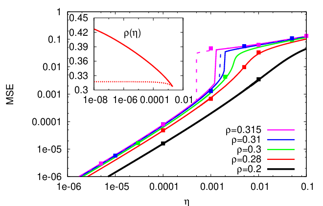

The potential (8) is shown in Fig. 1. Maximizing the potential, one obtains the Bayes-optimal MSE which we show in Fig. 2 as a function of for different densities . We see a phenomenology similar to that described in [13, 16] for other types of noise. Because of a two-maxima shape of the function , the Bayes-optimal MSE displays a sharp transition separating a region of parameters with a small MSE, comparable to , from a region with a large value of the MSE. In this second region of parameters compressed sensing technics –regardless of the reconstruction method– will not be useful. This is a “first order” phase transition.
Another important transition (the “spinodal”) that can be studied from the form of the potential function is the appearance of a high-MSE local maxima. Since the AMP algorithm performs a steepest ascent in the function (see e.g. [13]) this transition separates the region of parameters in which the performance of AMP will be asymptotically optimal from the one where AMP is suboptimal. An important feature of this transition, shown in Fig. 3, is that its position is only very weakly dependent on the value of the matrix uncertainty. This means that the performance of AMP is extremely robust to matrix uncertainty . The same result was also obtained for additive measurement noise in [13] and for approximate sparsity in [16].
4 Robust Message-Passing algorithm
The Bayesian approach to compressed sensing combined with belief propagation based reconstruction algorithm leads to the so-called approximate message passing (AMP) algorithm as first derived in [6] for the minimization of , and subsequently generalized in [18, 7, 13]. This approach was adapted by Parker, Cevher and Schniter to treat the matrix uncertainty MU-AMP in [5]. Here we shall consider a version of the canonical AMP, that we call robust-AMP, that turns out to be robust to noisy measurement and matrix uncertainty, so that it can be used indifferently of the presence or absence of noise and matrix uncertainty. We show in the next section that robust-AMP and MU-AMP are equivalent in the limit of infinite systems.
For every measurement component we define one real number , for each signal component we define four real numbers , , , . These quantities are updated as follows (for the derivation with these notations see [13]):
| (10) | |||||
| (11) | |||||
| (12) | |||||
| (13) | |||||
| (14) | |||||
| (15) |
Where only the functions and depend explicitly on the model :
| (16) | |||||
| (17) |
where is the following probability distribution
| (18) |
The explicit expression for and for the Gauss-Bernoulli signal is given in [13] while the case of approximate sparsity was considered in [16]. The above equations are initialized with , , , then the equations are iterated till convergence.
The difference between the present algorithm with respect to the more common version of AMP is in the way the estimate of the current error on the measurement element is computed in eq. (10). Most previous works (e.g. [7, 13]) used a -dependent vector in the case of noisy measurement with a perfectly known matrix, whereas the original paper [6] used a value precomputed by the state evolution. The modification done by the authors of ref. [5] to incorporate the effect of matrix uncertainty is (in our notation) . As shown in ref. [5] this leads to a very efficient algorithm with matrix uncertainty. The expression we use instead in eq. (10) was also proposed in [6]. Perhaps surprisingly, it is equivalent to the one of ref. [5] when the system size even in the case of matrix uncertainty. The advantage of expression (10) is that it is not need to explicitly know the value of and 11 1 Of course and can be learned with expectation maximization within the MU-AMP [8, 13, 15], but this adds considerable computational time.: the algorithm automatically incorporates the errors coming from the uncertainty on the matrix and the measurement; and hence we are using the same code regardless the presence or absence of noise and/or matrix uncertainty. We thus refer to algorithm (10)-(15) as the “robust”-AMP.
5 Density Evolution
The AMP approach is amenable to asymptotic () analysis in the case of i.i.d. random measurement matrices using a method known as the “cavity method” (in statistical physics) [9], the “density evolution” in coding [19], and the “state evolution” in the context of CS [6, 20]. We shall not detail the computation here, it goes in the same lines as in [13]. Given the parameters , , , , the MSE follows:
| (19) |
where follows eq. (8), with on the right hand side, , is a Gaussian integral, and is defined by eq. (17). The comparison between the evolution of the MSE in the algorithm and eq. (19) is shown on Fig. 4; the agreement is very good. Note that we have also applied the density evolution to the AMP algorithm with matrix uncertainty of [5], and found that it obeys asymptotically the same equation (19). More specifically, the term from eq. (10) evolves as in the limit both for the expression in ref. [5] and in eq. (10).

From eq. (19), one can also derive that the evolution is equivalent to a steepest ascent of the potential obtained from the replica method in eq. (8). This underlines the importance of the spinodal transition illustrated on Figs. 1, 2, and 3. In particular we see that the region where the AMP converges to the Bayes-optimal value of the MSE is quite large, and notably larger than the region in which the minimization is able to give precise reconstruction. Another point worth noting is that the location of the spinodal depends only very weakly to the value of the noise, for a large range of matrix and measurement noise (see inset of Fig. 2 and Fig. 3): this shows that the robust from of the AMP algorithm is indeed robust to noise(s).
6 Conclusions
We have computed the Bayes-optimal value of the MSE for the reconstruction of sparse Gauss-Bernoulli signals in presence of matrix uncertainty with the replica method, and consider a variant of the AMP algorithm robust to such uncertainty and to measurement noise. Finally, we have shown that AMP allows one to match the optimum MSE in a large region of parameters, and that the region is very weakly sensitive to measurement or matrix noises. Note that the present analysis applies to random i.i.d. measurement matrices; it is also possible to use the seeded spatially coupled measurement matrices of [8, 13, 14] and this would lead to an even larger region of optimality-matching performance for AMP.
References
- [1] E. J. Candès and T. Tao, “Near-Optimal Signal Recovery From Random Projections: Universal Encoding Strategies?,” IEEE Trans. Inform. Theory, vol. 52, pp. 5406, 2006.
- [2] D. L. Donoho, “Compressed sensing,” IEEE Trans. Inform. Theory, vol. 52, pp. 1289, 2006.
- [3] H. Zhu, G. Leus, and G. Giannakis, “Sparsity-cognizant total leastsquares for perturbed compressive sampling,” IEEE Transactions on Signal Processing, vol. 59, no. 5, pp. 2002––2016, 2011.
- [4] M. Rosenbaum and A. Tsybakov, “Sparse recovery under matrix uncertainty,” The Annals of Statistics, vol. 38, no. 5, pp. 2620––2651, 2010.
- [5] J.T. Parker, V. Cevher, and P. Schniter, “Compressive sensing under matrix uncertainties: An approximate message passing approach,” in Conference Record of the Forty Fifth Asilomar, 2011.
- [6] David L. Donoho, Arian Maleki, and Andrea Montanari, “Message-passing algorithms for compressed sensing,” Proc. Natl. Acad. Sci., vol. 106, no. 45, pp. 18914–18919, 2009.
- [7] S. Rangan, “Generalized approximate message passing for estimation with random linear mixing,” in IEEE International Symposium on Information Theory Proceedings (ISIT), 31 2011-aug. 5 2011, pp. 2168 –2172.
- [8] F. Krzakala, M. Mézard, F. Sausset, Y.F. Sun, and L. Zdeborová, “Statistical physics-based reconstruction in compressed sensing,” Phys. Rev. X, vol. 2, pp. 021005, 2012.
- [9] M. Mézard, G. Parisi, and M. A. Virasoro, Spin-Glass Theory and Beyond, vol. 9 of Lecture Notes in Physics, World Scientific, Singapore, 1987.
- [10] S. Rangan, A.K. Fletcher, and V. Goyal, “Asymptotic analysis of map estimation via the replica method and applications to compressed sensing,” arXiv:0906.3234v2, 2009.
- [11] Dongning Guo, D. Baron, and S. Shamai, “A single-letter characterization of optimal noisy compressed sensing,” in 47th Annual Allerton Conference on Communication, Control, and Computing, 2009, pp. 52 – 59.
- [12] Y. Kabashima, T. Wadayama, and T. Tanaka, “A typical reconstruction limit of compressed sensing based on lp-norm minimization,” J. Stat. Mech., p. L09003, 2009.
- [13] F. Krzakala, M. Mézard, F. Sausset, Y.F. Sun, and L. Zdeborová, “Probabilistic reconstruction in compressed sensing: Algorithms, phase diagrams, and threshold achieving matrices,” J. Stat. Mech., vol. P08009, 2012.
- [14] David L. Donoho, Adel Javanmard, and Andrea Montanari, “Information-theoretically optimal compressed sensing via spatial coupling and approximate message passing,” in Proc. of the IEEE Int. Symposium on Information Theory (ISIT), 2012.
- [15] J. P. Vila and P. Schniter, “Expectation-maximization bernoulli-gaussian approximate message passing,” in Proc. Asilomar Conf. on Signals, Systems, and Computers (Pacific Grove, CA), 2011.
- [16] J. Barbier, F. Krzakala, M. Mézard, and L. Zdeborová, “Compressed sensing of approximately-sparse signals: Phase transitions and optimal reconstruction,” in 50th Annual Allerton Conference on Communication, Control, and Computing, 2012.
- [17] David L. Donoho and Jared Tanner, “Sparse nonnegative solution of underdetermined linear equations by linear programming,” Proceedings of the National Academy of Sciences of the United States of America, vol. 102, no. 27, pp. 9446–9451, 2005.
- [18] D.L. Donoho, A. Maleki, and A. Montanari, “Message passing algorithms for compressed sensing: I. motivation and construction,” in Information Theory Workshop (ITW), 2010 IEEE, 2010, pp. 1 –5.
- [19] Tom Richardson and Rüdiger Urbanke, Modern Coding Theory, Cambridge University Press, 2008.
- [20] M. Bayati and A. Montanari, “The dynamics of message passing on dense graphs, with applications to compressed sensing,” IEEE Transactions on Information Theory, vol. 57, no. 2, pp. 764 –785, 2011.