跳到论文正文
W Papers独立论文阅读器 arXiv:1301.0881 论文正文 计算阅读时间 · 0%
引用这篇论文根据当前论文元数据生成,正式投稿前建议核对。


License: arXiv.org perpetual non-exclusive license
arXiv:1301.0881v2 [hep-ph] 30 May 2013

MZ-TH/12-55

December 2012

Fully analytical O⁡(αs)O(\alpha_{s}) results for on-shell and off-shell
polarized WW-boson decays into massive quark pairs
S. Groote1,2, J.G. Körner2 and P. Tuvike1
1 Loodus- ja Tehnoloogiateaduskond, Füüsika Instituut,

Tartu Ülikool, Tähe 4, 51010 Tartu, Estonia

2PRISMA Cluster of Excellence, Institut für Physik, Johannes-Gutenberg-Universität,

Staudinger Weg 7, 55099 Mainz, Germany

Abstract

We provide analytical O⁡(αs)O(\alpha_{s}) results for the three polarized decay structure functions H+⁣+,H00H_{++},\,H_{00} and H−⁣−H_{--} that describe the decay of a polarized WW boson into massive quark–antiquark pairs. As an application we consider the decay t→b+W+t\to b+W^{+} involving the helicity fractions ρm​m\rho_{mm} of the W+W^{+} boson followed by the polarized decay W+(↑)→q1​q¯2\hbox{$W^{+}(\uparrow)$}\to q_{1}\bar{q}_{2} described by the polarized decay structure functions Hm​mH_{mm}. We thereby determine the O⁡(αs)O(\alpha_{s}) polar angle decay distribution of the cascade decay process t→b+W+(→q1q¯2)t\to b+W^{+}(\to q_{1}\bar{q}_{2}). As a second example we analyze quark mass and off-shell effects in the cascade decays H→W−+W∗⁣+(→q1q¯2)H\to W^{-}+W^{\ast+}(\to q_{1}\bar{q}_{2}) and H→Z+Z∗(→qq¯)H\to Z+Z^{\ast}(\to q\bar{q}). For the decays H→W−+W∗⁣+(→cb¯)H\to W^{-}+W^{\ast+}(\to c\bar{b}) and H→Z+Z∗(→bb¯)H\to Z+Z^{\ast}(\to b\bar{b}) we find substantial deviations from the mass-zero approximation in particular in the vicinity of the threshold region.

1 Introduction

The polarization of W±W^{\pm} bosons produced in electroweak production processes is in general highly nontrivial. Therefore, the W±W^{\pm} bosons produced e.g. in p​p​(p​p¯)→W±+Xpp(p\bar{p})\to W^{\pm}+X, p​p​(p​p¯)→W+​W−+Xpp(p\bar{p})\to W^{+}W^{-}+X, e+​e−→W+​W−,W+​W−+Xe^{+}e^{-}\to W^{+}W^{-},\,W^{+}W^{-}+X and t→b+W+t\to b+W^{+} in general have a highly nontrivial polarization density matrix. Because of this, there is a rich phenomenology of polarization effects in WW production and decay to be explored in present and future experiments. For example, one would want to compare the results of polarization measurements with the predictions of the Standard Model (SM) or models beyond the SM.

The polarization of the W±W^{\pm} bosons can be probed by decay correlations involving the decay products of the polarized W±W^{\pm} boson. Using such decay correlations, first measurements of the W±W^{\pm} polarization in p​p→W±+Xpp\to W^{\pm}+X were reported by the CMS Collaboration [1] and the ATLAS Collaboration [2]. Measurements of the W±W^{\pm} polarization in e+​e−→W+​W−e^{+}e^{-}\to W^{+}W^{-} were published in Refs. [3, 4]. Finally, results of W+W^{+}-polarization measurements in t→b+W+t\to b+W^{+} were presented e.g. in Refs. [5, 6, 7, 8, 9, 10]. Ref. [11] provides a survey of SM expectations for the polarization of WW bosons in various production channels at the LHC.

In the SM the W±W^{\pm} boson decays into quark or lepton pairs. For unpolarized W±W^{\pm}-boson decays the NLO QCD and electroweak corrections to quark and lepton pair production, resp., have been given in Ref. [12, 13]. The radiative corrections in Ref. [12, 13] include also quark and lepton-mass effects. To our knowledge the radiative corrections to polarized W±W^{\pm}-boson decays including lepton and quark mass effects have not been done up to now.

This paper is devoted to the evaluation of the NLO QCD corrections to the decays of polarized W±W^{\pm} bosons into massive quark–antiquark pairs W±(↑)→q1q¯2W^{\pm}(\uparrow)\to q_{1}\,\bar{q}_{2} where the diagonal spin density matrix elements of the W±W^{\pm} boson can be probed through the polar angle decay distribution of the final-state quark pair. We augment our results such that they can also be applied to the decay of polarized ZZ decays into massive quark pairs. In order to provide quick access to the importance of quark mass effects in the decays of the W±W^{\pm} and ZZ bosons we have provided a O⁡(mqi2/mW2)O(m_{q_{i}}^{2}/m_{W}^{2}) quark mass expansions of our analytical results in a separate paper [14]. In a sequel to the present paper we shall calculate the corresponding NLO electroweak corrections to the polarized decay W+(↑)→ℓ+νℓW^{+}(\uparrow)\to\ell^{+}\,\nu_{\ell} [15].

In the limit mqi=:mi→0m_{q_{i}}=:m_{i}\to 0 our results reduce to rather simple forms which agree with previous NLO QCD results extracted from the corresponding calculation of (γ∗,Z)(↑)→qq¯(\gamma^{*},Z)(\uparrow)\to q\bar{q} [16, 17, 18, 19, 20]. Quark mass effects are non-negligible even for on-shell WW bosons with q2=mW2q^{2}=m_{W}^{2} for the polarized decay W+(↑)→cb¯W^{+}(\uparrow)\to c\bar{b} but become even more important for lower values of q2q^{2} as for the decays of off-shell W∗⁣±W^{\ast\pm} and Z∗Z^{\ast} bosons as they appear e.g. in the recently observed discovery channels H→W±​W∗⁣∓H\to W^{\pm}W^{\ast\mp} and H→Z​Z∗H\to ZZ^{\ast} of a 126​GeV126{\rm\,GeV} Higgs boson [21, 22]. Similarly one needs to retain mass effects in the calculation of current–current correlators and their corresponding spectral functions which are needed for all values of q2q^{2}. Since there have been claims and counterclaims in the literature as to the correctness of known results on radiative corrections to scalar (pseudoscalar) and vector (axial-vector) current–current spectral functions, we have compared our unpolarized results with previously published spectral function results.

As an illustration of our general decay analysis we consider the cascade decay process t→b+W+t\to b+W^{+} followed by W+→q1​q¯2W^{+}\to q_{1}\,\bar{q}_{2} where the (helicity frame) diagonal density matrix elements of the W+W^{+} boson resulting from the decay process t→b+W+t\to b+W^{+} have been well studied in the literature. We thus provide results on the angular decay distribution for the sequential cascade decay t→b+W+(→q1q¯2)t\to b+W^{+}(\to q_{1}\,\bar{q}_{2}) for which we discuss NLO QCD radiative corrections in the production process t→b+W+(↑)t\to b+W^{+}(\uparrow) and in the decay process W+(↑)→q1q¯2W^{+}(\uparrow)\to q_{1}\,\bar{q}_{2}. As a second example of much topical interest we take the cascade decay processes H→W−+W∗⁣+(→q1q¯2)H\to W^{-}+W^{\ast+}(\to q_{1}\bar{q}_{2}) and H→Z+Z∗(→qq¯)H\to Z+Z^{\ast}(\to q\bar{q}) where we discuss quark mass and W∗W^{\ast} and Z∗Z^{\ast} off-shell effects on rates and on angular decay distributions.

We also briefly comment on the nondiagonal density matrix elements of the W±W^{\pm} boson which can be probed by azimuthal correlations in the angular decay distribution. A measurement of the azimuthal correlations requires the existence of a preferred transverse direction which would be provided e.g. by the transverse polarization direction of the polarized top quark in the decay t(↑)→b+W+(→q1q¯2)t(\uparrow)\to b+W^{+}(\to q_{1}\,\bar{q}_{2}). In a similar vein a transverse direction can be defined in the large-pTp_{T} WW-boson production in the process p​p​(p​p¯)→W+Xpp(p\bar{p})\to W+X.

2 Born-term results

Let us consider the quark–antiquark decay of the SM gauge boson W+W^{+}

W+​(q)→q1​(p1)​q¯2​(p2)W^{+}(q)\to q_{1}(p_{1})\,\bar{q}_{2}(p_{2}) (1)

as depicted in Fig. 1.

Refer to captionRefer to caption

(a)                 (b)

Figure 1: Feynman diagrams for (a) the Born-term contribution and (b) the one-loop QCD contribution to the decay process W+→q1​q¯2W^{+}\to q_{1}\,\bar{q}_{2}

The LO Born-term amplitude is given by

ℳ⁡(𝐵𝑜𝑟𝑛)=ℳμ​(𝐵𝑜𝑟𝑛)​εμ​(q)=−i​gw2​Vi​j​u¯1​(p1)​γμ​1−γ52​v2​(p2)​εμ​(q),{\cal M}({\it Born\/})={\cal M}^{\mu}({\it Born\/})\varepsilon_{\mu}(q)=-i\frac{g_{w}}{\sqrt{2}}V_{ij}\,\,\bar{u}_{1}(p_{1})\gamma^{\mu}\frac{1-\gamma_{5}}{2}v_{2}(p_{2})\,\varepsilon_{\mu}(q), (2)

where gwg_{w} is the electroweak coupling constant and the Vi​jV_{ij} are Kobayashi–Maskawa matrix elements (q1=iq_{1}=i; q2=jq_{2}=j). We define a reduced matrix element ℳ~μ\widetilde{{\cal M}}^{\mu} by splitting off the common coupling factor −igWVi​j/2-ig_{W}V_{ij}/\sqrt{2} and the factor 1/21/2 from the chiral projector. The reduced Born-term tensor reads

Hμ​ν​(𝐵𝑜𝑟𝑛)\displaystyle H^{\mu\nu}({\it Born\/}) =\displaystyle= Nc​∑quark​spinsℳ~μ​(𝐵𝑜𝑟𝑛)​ℳ~†ν​(𝐵𝑜𝑟𝑛)\displaystyle N_{c}\sum_{\rm quark\ spins}\widetilde{{\cal M}}^{\mu}({\it Born\/})\widetilde{{\cal M}}^{\dagger\nu}({\it Born\/}) (3)
=\displaystyle= NcTr((p/1+m1)γμ(1−γ5)(p/2−m2)γν(1−γ5))\displaystyle N_{c}\,\mathop{\rm Tr}\nolimits\left((p\kern-5.0pt/_{1}+m_{1})\gamma^{\mu}(1-\gamma_{5})(p\kern-5.0pt/_{2}-m_{2})\gamma^{\nu}(1-\gamma_{5})\right)
=\displaystyle= 8​Nc​(p1μ​p2ν+p1ν​p2μ−p1​p2​gμ​ν+i​εμ​ν​α​β​p1​α​p2​β).\displaystyle 8N_{c}\left(p_{1}^{\mu}p_{2}^{\nu}+p_{1}^{\nu}p_{2}^{\mu}-p_{1}p_{2}\,g^{\mu\nu}+i\varepsilon^{\mu\nu\alpha\beta}p_{1\alpha}p_{2\beta}\right).

The Born-term amplitude (2) leads to the LO decay width for an on-shell W+W^{+} boson with q2=mW2q^{2}=m_{W}^{2} (gw2=4​π​α/sin2⁡θWg_{w}^{2}=4\pi\alpha/\sin^{2}\theta_{W}, μi=mi2/q2\mu_{i}=m_{i}^{2}/q^{2}),

Γ⁡(𝐵𝑜𝑟𝑛)\displaystyle\Gamma({\it Born\/}) =\displaystyle= 13​18​π​|p→|mW2​gw22​|Vi​j|2​Nc​Hμ​ν​(𝐵𝑜𝑟𝑛)​(−gμ​ν+qμ​qνmW2)\displaystyle\frac{1}{3}\,\frac{1}{8\pi}\,\frac{|\vec{p}|}{m_{W}^{2}}\frac{g_{w}^{2}}{2}|V_{ij}|^{2}N_{c}H_{\mu\nu}({\it Born\/})\left(-g_{\mu\nu}+\frac{q_{\mu}q_{\nu}}{m_{W}^{2}}\right) (4)
=\displaystyle= mW96​π​gW2​|Vi​j|2​Nc​λ​(2−μ1−μ2−(μ1−μ2)2),\displaystyle\frac{m_{W}}{96\pi}g_{W}^{2}|V_{ij}|^{2}N_{c}\,{\sqrt{\lambda}}\left(2-\mu_{1}-\mu_{2}-(\mu_{1}-\mu_{2})^{2}\right),

where |p→|=mW​λ/2|\vec{p}\,|=m_{W}{\sqrt{\lambda}}/2, and where λ\lambda is the value of the Källén function for the decay process,

λ=λ⁡(1,μ1,μ2)=1+μ12+μ22−2​μ1−2​μ2−2​μ1​μ2.\lambda=\lambda(1,\mu_{1},\mu_{2})=1+\mu_{1}^{2}+\mu_{2}^{2}-2\mu_{1}-2\mu_{2}-2\mu_{1}\mu_{2}. (5)

The rate expression (4) coincides with the Born-term result in Ref. [12].

The subject of this paper are the partial decays from states of the W+W^{+} boson with definite mm quantum numbers m=±1,0m=\pm 1,0, i.e. we are interested in the polarized decay structure functions

H±⁣±=Hμ​ν​εμ​(±)​ε∗ν​(±),H00=Hμ​ν​εμ​(0)​ε∗ν​(0).H_{\pm\pm}=H_{\mu\nu}\,\varepsilon^{\mu}(\pm)\varepsilon^{*\nu}(\pm),\qquad H_{00}=H_{\mu\nu}\,\varepsilon^{\mu}(0)\varepsilon^{*\nu}(0). (6)

We evaluate the polarized decay functions defined in Eq. (6) in the rest frame of the W+W^{+} boson with the z′z^{\prime} direction defined by the antiquark q¯2\bar{q}_{2}.11 1 We have chosen the antiquark direction to define the z′z^{\prime} axis in analogy to the antilepton ℓ+\ell^{+} in the decay W+→ℓ+​νℓW^{+}\to\ell^{+}\nu_{\ell}. One can equally well choose the quark to define the z′z^{\prime} axis. The resulting changes in the partial helicity rate functions will be discussed later on. The rest frame polarization vectors and momenta are thus given by

εμ​(±)\displaystyle\varepsilon^{\mu}(\pm) =\displaystyle= 12​(0,∓1,−i,0),qα=(mW,0,0,0),\displaystyle\frac{1}{\sqrt{2}}\,\Big(0;\mp 1,-i,0\Big),\qquad q^{\alpha}=\Big(m_{W};0,0,0\Big),
εμ​(0)\displaystyle\varepsilon^{\mu}(0) =\displaystyle= (0,0,0,1),p2α=(E2,0,0,|p→|),\displaystyle\Big(0;0,0,1\Big),\qquad\qquad p_{2}^{\alpha}=(E_{2};0,0,|\vec{p}\,|), (7)

where E2=mW​(1−μ1+μ2)/2E_{2}=m_{W}(1-\mu_{1}+\mu_{2})/2 and |p→|=q2​λ⁡(1,μ1,μ2)/2|\vec{p}\,|=\sqrt{q^{2}}\sqrt{\lambda(1,\mu_{1},\mu_{2})}/2.

It proves convenient to bring the rest frame projectors I​P±⁣±μ​ν=εμ​(±)​ε∗ν​(±)\mbox{I}\!\mbox{P}^{\mu\nu}_{\pm\pm}=\varepsilon^{\mu}(\pm)\varepsilon^{*\nu}(\pm) and I​P00μ​ν=εμ​(0)​ε∗ν​(0)\mbox{I}\!\mbox{P}^{\mu\nu}_{00}=\varepsilon^{\mu}(0)\varepsilon^{*\nu}(0) into a frame-independent covariant form. One has

I​P±⁣±μ​ν=12​(I​PU+Lμ​ν−I​PLμ​ν±I​PFμ​ν),I​P00μ​ν=I​PLμ​ν,\mbox{I}\!\mbox{P}^{\mu\nu}_{\pm\pm}\ =\ \frac{1}{2}\left(\mbox{I}\!\mbox{P}^{\mu\nu}_{U+L}-\mbox{I}\!\mbox{P}^{\mu\nu}_{L}\pm\mbox{I}\!\mbox{P}^{\mu\nu}_{F}\right),\qquad\mbox{I}\!\mbox{P}^{\mu\nu}_{00}\ =\ \mbox{I}\!\mbox{P}^{\mu\nu}_{L}, (8)

where

I​PU+Lμ​ν\displaystyle\mbox{I}\!\mbox{P}^{\mu\nu}_{U+L} =\displaystyle= −gμ​ν+qμ​qνq2,\displaystyle-g^{\mu\nu}+\frac{q^{\mu}q^{\nu}}{q^{2}},
I​PLμ​ν\displaystyle\mbox{I}\!\mbox{P}^{\mu\nu}_{L} =\displaystyle= q2NP2​(p2μ−p2⋅qq2​qμ)​(p2ν−p2⋅qq2​qν),\displaystyle\frac{q^{2}}{N_{P}^{2}}\Big(p_{2}^{\mu}-\frac{p_{2}\cdot q}{q^{2}}q^{\mu}\Big)\Big(p_{2}^{\nu}-\frac{p_{2}\cdot q}{q^{2}}q^{\nu}\Big),
I​PFμ​ν\displaystyle\mbox{I}\!\mbox{P}^{\mu\nu}_{F} =\displaystyle= 1NP​i​ϵμ​ν​α​β​p2​α​qβ,\displaystyle\frac{1}{N_{P}}i\epsilon^{\mu\nu\alpha\beta}p_{2\alpha}q_{\beta}, (9)

and where the normalization factor NPN_{P} is given by NP2=((p2​q)2−p22​q2)N_{P}^{2}=((p_{2}q)^{2}-p_{2}^{2}q^{2}). In the two-body case the normalization factor is reduced to NP=q2​|p→|N_{P}=\sqrt{q^{2}}\,|\vec{p}\,|. The covariant form of the projectors are particularly convenient in the NLO tree-graph calculation since the covariantly projected integrands in the requisite phase space integrations are Lorentz scalars and can thus be handled by the standard covariant methods.

Using either forms for the projectors (6) or (8), one obtains

H±⁣±​(𝐵𝑜𝑟𝑛)=4​Nc​q2​(1−μ1−μ2±λ),H00​(𝐵𝑜𝑟𝑛)=4​Nc​q2​(1−μ1−μ2−λ).H_{\pm\pm}({\it Born\/})=4N_{c}q^{2}(1-\mu_{1}-\mu_{2}\pm{\sqrt{\lambda}}),\qquad H_{00}({\it Born\/})=4N_{c}q^{2}(1-\mu_{1}-\mu_{2}-\lambda). (10)

Note that the sum HU=H+⁣++H−⁣−H_{U}=H_{++}+H_{--} (UU: unpolarized transverse) and HL=H00H_{L}=H_{00} (LL: longitudinal) are fed only by the parity-even V​VVV and A​AAA current products. The difference HF=H+⁣+−H−⁣−H_{F}=H_{++}-H_{--} (FF: forward–backward asymmetric) is fed by the parity-odd V​AV\!A current product.

At threshold, where q2→(m1+m2)2q^{2}\to(m_{1}+m_{2})^{2}, with μ1+μ2→1\sqrt{\mu_{1}}+\sqrt{\mu_{2}}\to 1 and λ→0\lambda\to 0, one has H−⁣−​(𝐵𝑜𝑟𝑛)=H00​(𝐵𝑜𝑟𝑛)=H+⁣+​(𝐵𝑜𝑟𝑛)=8​Nc​m1​m2H_{--}({\it Born\/})=H_{00}({\it Born\/})=H_{++}({\it Born\/})=8N_{c}m_{1}m_{2}. All three partial helicity rates are equal to one another at threshold. This can be understood from the fact that, at threshold, only the vector current-induced L​SLS amplitude (L​S)=(01)(LS)=(01) survives. This leads to the equality of the partial helicity rates using simple Clebsch–Gordan algebra. As we shall see in the next section, at threshold one loses the analyzing power of the two-fermion decay mode, i.e. the angular decay distribution becomes flat at threshold irrespective of the polarization of the W+W^{+} boson.

In the massless quark limit μ1=μ2=0\mu_{1}=\mu_{2}=0 one has H+⁣+​(𝐵𝑜𝑟𝑛)=8​Nc​q2≠0H_{++}({\it Born\/})=8N_{c}q^{2}\neq 0 and H00​(𝐵𝑜𝑟𝑛)=H−⁣−​(𝐵𝑜𝑟𝑛)=0H_{00}({\it Born\/})=H_{--}({\it Born\/})=0 as expected from the left-chiral nature of the SM current (2). The finite mass corrections to the LO helicity structure functions are of O⁡(μi)O(\mu_{i}) for H+⁣+H_{++} and H00H_{00}, i.e. H+⁣+​(𝐵𝑜𝑟𝑛)=8​Nc​q2​(1−μ1−μ2+…)H_{++}({\it Born\/})=8N_{c}q^{2}(1-\mu_{1}-\mu_{2}+\ldots) and H00​(𝐵𝑜𝑟𝑛)=4​Nc​q2​(μ1+μ2+…)H_{00}({\it Born\/})=4N_{c}q^{2}(\mu_{1}+\mu_{2}+\ldots), and of O⁡(μi2)O(\mu_{i}^{2}) for H−⁣−H_{--}, i.e. H−⁣−​(𝐵𝑜𝑟𝑛)=4​Nc​q2​(μ1​μ2+…)H_{--}({\it Born\/})=4N_{c}q^{2}(\mu_{1}\mu_{2}+\ldots). For the sum of the three polarized decay functions denoted by HU+LH_{U+L} one obtains

HU+L​(𝐵𝑜𝑟𝑛)\displaystyle H_{U+L}({\it Born\/}) =\displaystyle= H−⁣−​(𝐵𝑜𝑟𝑛)+H00​(𝐵𝑜𝑟𝑛)+H+⁣+​(𝐵𝑜𝑟𝑛)\displaystyle H_{--}({\it Born\/})+H_{00}({\it Born\/})+H_{++}({\it Born\/}) (11)
=\displaystyle= 12​Nc​q2​(1−μ1−μ2−λ/3).\displaystyle 12N_{c}q^{2}\left(1-\mu_{1}-\mu_{2}-\lambda/3\right).

For the sake of completeness we also define a scalar structure function Ht​tH_{tt} through Ht​t=Hμ​ν​εμ​(t)​ε∗ν​(t)H_{tt}=H_{\mu\nu}\,\varepsilon^{\mu}(t)\varepsilon^{*\nu}(t) where εμ​(t)=(1,0,0,0)\varepsilon^{\mu}(t)=(1;0,0,0) is the rest-frame time-component (scalar) polarization vector of the off-shell W+W^{+} boson. The corresponding covariant projector on the scalar structure function reads

I​PSμ​ν=qμ​qνq2.\mbox{I}\!\mbox{P}^{\mu\nu}_{S}=\frac{q^{\mu}q^{\nu}}{q^{2}}. (12)

For the LO scalar structure function one obtains

Ht​t​(𝐵𝑜𝑟𝑛)=HS​(𝐵𝑜𝑟𝑛)=4​Nc​q2​(1−μ1−μ2−λ).H_{tt}({\it Born\/})=H_{S}({\it Born\/})=4N_{c}q^{2}\left(1-\mu_{1}-\mu_{2}-\lambda\right). (13)

Note that, at the Born-term level, one has Ht​t​(𝐵𝑜𝑟𝑛)=H00​(𝐵𝑜𝑟𝑛)H_{tt}({\it Born\/})=H_{00}({\it Born\/}). Ht​t​(𝐵𝑜𝑟𝑛)H_{tt}({\it Born\/}) vanishes for zero quark masses as expected from current conservation in the mass-zero limit.

The scalar–longitudinal interference term needed later on is projected by

I​Pt​0μ​ν=1NP​qμ​(p2ν−p2⋅qq2​qν),\mbox{I}\!\mbox{P}^{\mu\nu}_{t0}=\frac{1}{N_{P}}q^{\mu}\,\Big(p_{2}^{\nu}-\frac{p_{2}\cdot q}{q^{2}}q^{\nu}\Big), (14)

such that

H0​t​(𝐵𝑜𝑟𝑛)=Ht​0​(𝐵𝑜𝑟𝑛)=−4​Nc​q2​(μ1−μ2)​λ.H_{0t}({\it Born\/})=H_{t0}({\it Born\/})=-4N_{c}q^{2}\left(\mu_{1}-\mu_{2}\right){\sqrt{\lambda}}. (15)

3 Angular decay distribution and
the cascade decay t→b+W+(→qiq¯j)t\to b+W^{+}(\to q_{i}\,\bar{q}_{j})

Consider the rest frame decay of a polarized W+W^{+} with the diagonal spin density matrix elements (ρ+⁣+,ρ00,ρ−⁣−\rho_{++},\rho_{00},\rho_{--}) given in an unprimed coordinate system (x,y,z)(x,y,z). Then rotate the coordinate system (x,y,z)(x,y,z) around the yy axis by an angle θ\theta to a primed coordinate system (x′,y,z′)(x^{\prime},y,z^{\prime}). Under this rotation the diagonal density matrix elements transform according to ρm′​m′′​(θ)=ρm​m​dm​m′1​(θ)​dm​m′1​(θ)\rho^{\prime}_{m^{\prime}m^{\prime}}(\theta)=\rho_{mm}\,d^{1}_{mm^{\prime}}(\theta)d^{1}_{mm^{\prime}}(\theta). The angular decay distribution is then determined by the product of the decay probability Hm′​m′H_{m^{\prime}m^{\prime}} for the decay W+​(m′)→q1​q¯2W^{+}(m^{\prime})\to q_{1}\,\bar{q}_{2} and the relevant diagonal elements of the spin density matrix elements ρm′​m′′​(θ)\rho^{\prime}_{m^{\prime}m^{\prime}}(\theta), all evaluated in the primed system.

While a decay analysis in the W+W^{+} rest system is the optimal choice to probe the density matrix elements of the W+W^{+} boson, the polarization of the W+W^{+} boson can also be detected in other coordinate systems. As an example take the cascade decay t→b+W+(→ℓ+νℓ)t\to b+W^{+}(\to\ell^{+}\,\nu_{\ell}). When analyzed in the top quark rest system, the polarization of the W+W^{+} will affect the energy spectrum of the final lepton, i.e. leptons from ρ−⁣−\rho_{--} will be more energetic than those from ρ+⁣+\rho_{++}.

Returning to the analysis in the W+W^{+} rest frame we mention that the choice of the zz and z′z^{\prime} axes is a matter of convention and convenience and may be dictated by the physics at hand. For example, in the process p​p​(p​p¯)→W++Xpp(p\bar{p})\to W^{+}+X followed by W+→ℓ+​νW^{+}\to\ell^{+}\nu several unprimed rest frame coordinate systems have been discussed in the literature (Collins–Soper frame, recoil frame, target frame, beam frame) whereas the z′z^{\prime} direction is conventionally fixed by the lepton direction.22 2 NLO results on WW polarization effects in p​p¯→W+Xp\bar{p}\to W+X can be found in Refs. [23, 24].

In the example discussed further on (t→b+W+(→q1q¯2)t\to b+W^{+}(\to q_{1}\,\bar{q}_{2})) the zz direction is fixed by the momentum direction of the W+W^{+} in the top quark rest system (helicity system), and the z′z^{\prime} direction is determined by the momentum direction of the antiquark q¯2\bar{q}_{2}.

It is convenient to work in terms of normalized spin density matrix elements defined by ρ^m​m=ρm​m/∑m′ρm′​m′\hat{\rho}_{mm}=\rho_{mm}/\sum_{m^{\prime}}\rho_{m^{\prime}m^{\prime}} with ρ^+⁣++ρ^00+ρ^−⁣−=1\hat{\rho}_{++}+\hat{\rho}_{00}+\hat{\rho}_{--}=1 and normalized decay functions given by H^m​m=Hm​m/∑m′Hm′​m′\hat{H}_{mm}=H_{mm}/\sum_{m^{\prime}}H_{m^{\prime}m^{\prime}} such that H^+⁣++H^00+H^−⁣−=1\hat{H}_{++}+\hat{H}_{00}+\hat{H}_{--}=1. According to what was said before, the normalized decay distribution is given by

W^​(θ)\displaystyle\widehat{W}(\theta) =\displaystyle= 32∑m,m′=0,±ρ^m​m​dm​m′1​(θ)​dm​m′1​(θ)​H^m′​m′\displaystyle\frac{3}{2}\quad\sum_{m,m^{\prime}=0,\pm}\hat{\rho}_{mm}\,d^{1}_{mm^{\prime}}(\theta)\,d^{1}_{mm^{\prime}}(\theta)\,\hat{H}_{m^{\prime}m^{\prime}} (16)
=\displaystyle= 38​(1+cos2⁡θ)​(ρ^+⁣++ρ^−⁣−)​(H^+⁣++H^−⁣−)+34​cos⁡θ⁡(ρ^+⁣+−ρ^−⁣−)​(H^+⁣+−H^−⁣−)\displaystyle\frac{3}{8}(1+\cos^{2}\theta)\,(\hat{\rho}_{++}+\hat{\rho}_{--})\,(\hat{H}_{++}+\hat{H}_{--})+\frac{3}{4}\cos\theta\,(\hat{\rho}_{++}-\hat{\rho}_{--})\,(\hat{H}_{++}-\hat{H}_{--})
+34​sin2⁡θ⁡(ρ^+⁣+​H^00+ρ^00​H^+⁣++ρ^00​H^−⁣−+ρ^−⁣−​H^00)+32​cos2⁡θ​ρ^00​H^00\displaystyle+\frac{3}{4}\sin^{2}\theta\,(\hat{\rho}_{++}\,\hat{H}_{00}+\hat{\rho}_{00}\,\hat{H}_{++}+\hat{\rho}_{00}\,\hat{H}_{--}+\hat{\rho}_{--}\,\hat{H}_{00})+\frac{3}{2}\cos^{2}\theta\,\hat{\rho}_{00}\,\hat{H}_{00}
=\displaystyle= 38​cos2⁡θ⁡(ρ^+⁣+−2​ρ^00+ρ^−⁣−)​(H^+⁣+−2​H^00+H^−⁣−)\displaystyle\frac{3}{8}\cos^{2}\theta\,(\hat{\rho}_{++}-2\hat{\rho}_{00}+\hat{\rho}_{--})(\hat{H}_{++}-2\hat{H}_{00}+\hat{H}_{--})
+34​cos⁡θ⁡(ρ^+⁣+−ρ^−⁣−)​(H^+⁣+−H^−⁣−)\displaystyle+\frac{3}{4}\cos\theta(\hat{\rho}_{++}-\hat{\rho}_{--})\,(\hat{H}_{++}-\hat{H}_{--})
+38​((ρ^+⁣++2​ρ^00+ρ^−⁣−)​(H^+⁣++2​H^00+H^−⁣−)−4​ρ^00​H^00).\displaystyle+\frac{3}{8}\Big((\hat{\rho}_{++}+2\hat{\rho}_{00}+\hat{\rho}_{--})(\hat{H}_{++}+2\hat{H}_{00}+\hat{H}_{--})-4\hat{\rho}_{00}\hat{H}_{00}\Big).

The distribution (16) is a second-degree polynomial in cos⁡θ\cos\theta and therefore has the form of a parabola. Integrating over cos⁡θ\cos\theta one obtains

∫W^​(θ)​d​cos⁡θ=1.\int\widehat{W}(\theta)\,d\cos\theta=1. (17)

For unpolarized W+W^{+} decay one has ρ^−⁣−=ρ^00=ρ^+⁣+=1/3\hat{\rho}_{--}=\hat{\rho}_{00}=\hat{\rho}_{++}=1/3 which results in a flat decay distribution W^​(θ)=1/2\widehat{W}(\theta)=1/2. Similarly, one obtains a flat decay distribution at threshold where H^−⁣−=H^00=H^+⁣+=1/3\hat{H}_{--}=\hat{H}_{00}=\hat{H}_{++}=1/3, i.e. W^​(θ)∝(ρ^−⁣−+ρ^00+ρ^+⁣+)/2=1/2\widehat{W}(\theta)\propto(\hat{\rho}_{--}+\hat{\rho}_{00}+\hat{\rho}_{++})/2=1/2 irrespective of the polarization of the WW boson.

In the zero quark mass limit and to leading order in αs\alpha_{s} (where H^+⁣+​(𝐵𝑜𝑟𝑛)=1\hat{H}_{++}({\it Born\/})=1 and H^00​(𝐵𝑜𝑟𝑛)=H^−⁣−​(𝐵𝑜𝑟𝑛)=0\hat{H}_{00}({\it Born\/})=\hat{H}_{--}({\it Born\/})=0) the angular decay distribution (16) reduces to

W^​(θ)=38​(1+cos⁡θ)2​ρ^+⁣++38​(1−cos⁡θ)2​ρ^−⁣−+34​sin2⁡θ​ρ^00,\widehat{W}(\theta)\ =\ \frac{3}{8}(1+\cos\theta)^{2}\,\hat{\rho}_{++}+\frac{3}{8}(1-\cos\theta)^{2}\,\hat{\rho}_{--}+\frac{3}{4}\sin^{2}\theta\,\hat{\rho}_{00}, (18)

a form quite familiar from the analysis of the cascade decay t→b+W+(→νμμ+)t\to b+W^{+}(\to\nu_{\mu}\,\mu^{+}) [5, 6, 7, 8, 9].

Let us now turn to the αs\alpha_{s} corrections to the polarized decay functions Hm​mH_{mm} where we include quark mass effects. Surprisingly it turns out that the quark mass corrections to the leading NLO term set in linearly and carry rather large coefficients. This has to be contrasted with the LO and the NLO unpolarized decay term where the mass corrections set in quadratically. In fact, expanding the O⁡(αs)O(\alpha_{s}) polarized decay functions Hm​mH_{mm} listed in Sec. 7 up to O⁡(μi)O(\sqrt{\mu_{i}}), one obtains (see also Ref. [14] where the expansion is carried out to O⁡(μi)O(\mu_{i}))

H+⁣+\displaystyle H_{++} =\displaystyle= 8​Nc​q2​[ 1+αs6​π​(1+(π2+16)​μ2)+…],\displaystyle 8N_{c}q^{2}\bigg[\,1+\frac{\alpha_{s}}{6\pi}\Big(1+(\pi^{2}+16)\sqrt{\mu_{2}}\Big)+\ldots\bigg],
H00\displaystyle H_{00}\,\,\, =\displaystyle= 8​Nc​q2​[ 0+αs6​π​(4−2​π2​μ2)+…],\displaystyle 8N_{c}q^{2}\bigg[\,0+\frac{\alpha_{s}}{6\pi}\Big(4-2\pi^{2}\sqrt{\mu_{2}}\Big)+\ldots\bigg],
H−⁣−\displaystyle H_{--} =\displaystyle= 8​Nc​q2​[ 0+αs6​π​(1+(π2−16)​μ2)+…].\displaystyle 8N_{c}q^{2}\bigg[\,0+\frac{\alpha_{s}}{6\pi}\Big(1+(\pi^{2}-16)\sqrt{\mu_{2}}\Big)+\ldots\bigg]. (19)

The NLO linear mass corrections are proportional to the antiquark mass m2m_{2} and are thus maximally asymmetric in the quark masses.33 3 When one chooses the z′z^{\prime} direction along the quark direction (called system I in Ref. [14]), the linear mass corrections are proportional to the quark mass m1m_{1}. As discussed in Ref. [14], the polarized decay functions Hm​mIH^{I}_{mm} in this system are obtained from the present results by the substitution H±⁣±I​I​(1,2)→H∓⁣∓I​(2,1)H^{II}_{\pm\pm}(1,2)\to H^{I}_{\mp\mp}(2,1) and H00I​I​(1,2)→H00I​(2,1)H^{II}_{00}(1,2)\to H^{I}_{00}(2,1) where, using the notation of Ref. [14], the polarized decay functions described in this paper are denoted by Hm​mI​I​(1,2)H^{II}_{mm}(1,2). It is apparent that the NLO linear mass terms cancel in the sum H+⁣++H00+H−⁣−H_{++}+H_{00}+H_{--}. We mention that the leading order O⁡(μi0)O(\mu_{i}^{0}) αs\alpha_{s} contributions can also be extracted from the corresponding calculation of (γ∗,Z)(↑)→qq¯(\gamma^{*},Z)(\uparrow)\to q\bar{q} in Refs. [16, 17, 18, 19, 20] when the quark masses are set to zero in these calculations. As concerns the leading order αs\alpha_{s} contributions, the largest contribution occurs for H00H_{00} and amounts to 2​αs/(3​π)=2.5%2\alpha_{s}/(3\pi)=2.5\,\% with αs​(mW2)=0.117\alpha_{s}(m_{W}^{2})=0.117. The αs\alpha_{s} corrections can be seen to sum up to H+⁣++H00+H−⁣−∼(1+αs/π)H_{++}+H_{00}+H_{--}\sim(1+\alpha_{s}/\pi), a result which is well familiar from e+​e−e^{+}e^{-} annihilation into mass-zero quark pairs.

The NLO linear mass corrections have rather large coefficients. For example for W+→c​b¯W^{+}\to c\bar{b} and for the polarized structure function H+⁣+H_{++}, which is the only polarized structure function with a sizeable LO contribution, the linear mass correction amounts to 155%155\,\% (with mb=4.8​GeVm_{b}=4.8{\rm\,GeV} and mW=80.399​GeVm_{W}=80.399{\rm\,GeV}). However, the large mass corrections are tempered when one calculates the normalized decay functions H^m​m\hat{H}_{mm} which enter the normalized angular decay distribution. In fact, one obtains (H^+⁣++H^00+H^−⁣−=1\hat{H}_{++}+\hat{H}_{00}+\hat{H}_{--}=1)

H^+⁣+\displaystyle\hat{H}_{++} =\displaystyle= 1+αs6​π​(−5+(π2+16)​μ2)+…\displaystyle 1+\frac{\alpha_{s}}{6\pi}\left(-5+(\pi^{2}+16)\sqrt{\mu_{2}}\right)+\ldots
H^00\displaystyle\hat{H}_{00} =\displaystyle= 0+αs6​π​(4−2​π2​μ2)+…\displaystyle 0+\frac{\alpha_{s}}{6\pi}\left(4-2\pi^{2}\sqrt{\mu_{2}}\right)+\ldots
H^−⁣−\displaystyle\hat{H}_{--} =\displaystyle= 0+αs6​π​(1+(π2−16)​μ2)+…\displaystyle 0+\frac{\alpha_{s}}{6\pi}\left(1+(\pi^{2}-16)\sqrt{\mu_{2}}\right)+\ldots (20)

where we have used a small αs\alpha_{s} expansion for the ratios Hm​m/HU+LH_{mm}/H_{U+L}. For W+→c​b¯W^{+}\to c\bar{b} the linear NLO quark mass effects now amount to only O⁡(35%)O(35\,\%) of the leading NLO contribution. The reason for the reduction of the linear mass effects is that the largest linear mass effect resides in the (unnormalized) polarized decay function H+⁣+H_{++} which has a sizeable LO contribution.

The normalized angular decay distribution (16) can be characterized by the convexity parameter (see e.g. Ref. [14])

cf=d2​W^​(θ)d​(cos⁡θ)2=34​(ρ^+⁣+−2​ρ^00+ρ^−⁣−)​(H^+⁣+−2​H^00+H^−⁣−).c_{f}=\frac{d^{2}\widehat{W}(\theta)}{d(\cos\theta)^{2}}=\frac{3}{4}(\hat{\rho}_{++}-2\hat{\rho}_{00}+\hat{\rho}_{--})(\hat{H}_{++}-2\hat{H}_{00}+\hat{H}_{--}). (21)

When cfc_{f} is negative (positive), the angular decay distribution is described by a downward (upward) open parabola. As a second global measure we introduce the forward–backward asymmetry of the decay distribution defined by

AF​B=W⁡(F)−W⁡(B)W⁡(F)+W⁡(B)=34​(ρ^+⁣+−ρ^−⁣−)​(H^+⁣+−H^−⁣−),A_{FB}=\frac{W(F)-W(B)}{W(F)+W(B)}=\frac{3}{4}(\hat{\rho}_{++}-\hat{\rho}_{--})(\hat{H}_{++}-\hat{H}_{--}), (22)

where W⁡(F)=W⁡(0≤θ≤π/2)W(F)=W(0\leq\theta\leq\pi/2) and W⁡(B)=W⁡(π/2≤θ≤π)W(B)=W(\pi/2\leq\theta\leq\pi). If there is an extremum of the angular decay distribution in the physical range −1≤cos⁡θ≤1-1\leq\cos\theta\leq 1, the extremum is given by

cos⁡θ|extr=−AF​Bcf=−(ρ^+⁣+−ρ^−⁣−)(ρ^+⁣+−2​ρ^00+ρ^−⁣−)​(H^+⁣+−H^−⁣−)(H^+⁣+−2​H^00+H^−⁣−).\cos\theta\,\Big|_{\,\rm extr}=-\frac{A_{FB}}{c_{f}}=\,-\ \frac{(\hat{\rho}_{++}-\hat{\rho}_{--})}{(\hat{\rho}_{++}-2\hat{\rho}_{00}+\hat{\rho}_{--})}\ \frac{(\hat{H}_{++}-\hat{H}_{--})}{(\hat{H}_{++}-2\hat{H}_{00}+\hat{H}_{--})}. (23)

The three measures are not independent since cosθ|extr=−AF​B/cf\cos\theta\,\Big|_{\,\rm extr}=\,-A_{FB}/c_{f}.

In the small αs\alpha_{s} expansion and neglecting quark mass effects one has

cf\displaystyle c_{f} =\displaystyle= 34​(1−3​ρ^00)​(1−12​αs6​π),\displaystyle\frac{3}{4}(1-3\hat{\rho}_{00})(1-12\,\frac{\alpha_{s}}{6\pi}), (24)
AF​B\displaystyle A_{FB} =\displaystyle= −34​(ρ^+⁣+−ρ^−⁣−)​(1−6​αs6​π),\displaystyle-\frac{3}{4}(\hat{\rho}_{++}-\hat{\rho}_{--})(1-6\,\frac{\alpha_{s}}{6\pi}), (25)
cos⁡θ|extr\displaystyle\cos\theta\,\Big|_{\,\rm extr} =\displaystyle= (ρ^+⁣+−ρ^−⁣−)(1−3​ρ^00)​(1+6​αs6​π).\displaystyle\ \frac{(\hat{\rho}_{++}-\hat{\rho}_{--})}{(1-3\hat{\rho}_{00})}(1+6\,\frac{\alpha_{s}}{6\pi}). (26)

The largest αs\alpha_{s} correction occurs for the convexity parameter cfc_{f}. Using αs​(mW2)=0.117\alpha_{s}(m^{2}_{W})=0.117 one finds a 7.5%7.5\,\% reduction of cfc_{f} through the radiative corrections, i.e. the radiatively corrected angular decay distribution becomes flatter by that amount. This flattening is clearly discernible in the plot of the cos⁡θ\cos\theta distribution of the decay shown in Sec. 8.

Let us now for illustrative purposes turn to a specific example, namely the cascade decay t→b+W+(→q1q¯2)t\to b+W^{+}(\to q_{1}\,\bar{q}_{2}). This process is particularly interesting since the NLO radiative QCD corrections factorize into initial- and final-state corrections, i.e. there is no NLO cross talk between top quark decay and WW decay because of colour conservation [25].

The spin density matrix elements of the W+W^{+} in the decay process t→b+W+t\to b+W^{+} are well studied. At LO one has [26]

ρ^+⁣+​(𝐵𝑜𝑟𝑛)\displaystyle\hat{\rho}_{++}({\it Born\/}) =\displaystyle= 0→  0.0007,\displaystyle 0\qquad\qquad\qquad\qquad\quad\to\,\,0.0007,
ρ^00​(𝐵𝑜𝑟𝑛)\displaystyle\hat{\rho}_{00}({\it Born\/}) =\displaystyle= 11+2​x2=0.696→  0.6887,\displaystyle\frac{1}{1+2x^{2}}\ =0.696\qquad\,\to\,\,0.6887,
ρ^−⁣−​(𝐵𝑜𝑟𝑛)\displaystyle\hat{\rho}_{--}({\it Born\/}) =\displaystyle= 2​x21+2​x2= 0.304→  0.3106,\displaystyle\frac{2x^{2}}{1+2x^{2}}\ =\ 0.304\qquad\!\to\,\,0.3106, (27)

where x=mW/mtx=m_{W}/m_{t}. For the numerical values we use the central values of mW=80.399±0.025​GeVm_{W}=80.399\pm 0.025{\rm\,GeV} and mt=172.0±0.9±1.3​GeVm_{t}=172.0\pm 0.9\pm 1.3{\rm\,GeV} provided by the Particle Data Group [27]. At leading order the density matrix element ρ^+⁣+\hat{\rho}_{++} is not populated because of angular momentum conservation in the two-body decay process. In Eq. (27) we have also given the NLO QCD results indicated by arrows (cf. Refs. [28, 29, 30, 31]).44 4 The NNLO corrections to the spin density matrix elements of the W+W^{+} have recently been calculated in Ref. [32]. The correction to ρ^+⁣+\hat{\rho}_{++} is very small. The absolute corrections to ρ^00\hat{\rho}_{00} and ρ^−⁣−\hat{\rho}_{--} amount to 0.73%0.73\% and 0.66%0.66\% and are thus considerably smaller than the final-state mass-zero corrections to H^+⁣+\hat{H}_{++} and H^00\hat{H}_{00} given in Eq. (20).

If a transverse direction can be specified, one can also probe the nondiagonal spin density matrix elements ρ^m​m′\hat{\rho}_{mm^{\prime}} with m≠m′m\neq m^{\prime}. The angular decay distribution is then given by [33]

W⁡(θ)=∑m,m′,m′′ρ^m​m′​dm​m′′1​(θ)​dm′​m′′1​(θ)​Hm′′​m′′​e−i⁡(m−m′)​ϕ,W(\theta)=\sum_{m,m^{\prime},m^{\prime\prime}}\hat{\rho}_{mm^{\prime}}\,d^{1}_{mm^{\prime\prime}}(\theta)\,d^{1}_{m^{\prime}m^{\prime\prime}}(\theta)\,\,H_{m^{\prime\prime}m^{\prime\prime}}\,\,e^{-i(m-m^{\prime})\phi}, (28)

where ϕ\phi denotes the azimuthal angle between the production and decay plane. For m′≠mm^{\prime}\neq m there will be the typical pattern of dispersive and absorptive (or C​PCP violating) contributions proportional to cos⁡(m−m′)​ϕ\cos(m-m^{\prime})\,\phi and sin⁡(m−m′)​ϕ\sin(m-m^{\prime})\,\phi, respectively. We mention that, if one generalizes the above example t→b+W+(→q1q¯2)t\to b+W^{+}(\to q_{1}\,\bar{q}_{2}) to the decay of a polarized top quark t(↑)→b+W+(→q1q¯2)t(\uparrow)\to b+W^{+}(\to q_{1}\,\bar{q}_{2}), a production plane can be defined with the help of the transverse polarization of the top quark. The corresponding polar and azimuthal distributions are given in Refs. [28, 30]. A further example where the nondiagonal density matrix elements come into play is the much discussed decay H→f1​f¯2​f3​f¯4H\to f_{1}\bar{f}_{2}f_{3}\bar{f}_{4} treated e.g. in Ref. [34, 35] where one f​f¯f\bar{f} plane provides the reference transverse direction needed for the definition of the relative azimuthal orientation of the second plane.

4 One-loop contributions

For calculational reasons it is convenient to introduce linear combinations of the diagonal helicity structure functions H+⁣+H_{++}, H−⁣−H_{--} and H00H_{00} given by

H1=12​(H+⁣++H−⁣−),H2=12​(H+⁣+−H−⁣−),H3=12​(H+⁣++H−⁣−−2​H00).H_{1}=\frac{1}{2}(H_{++}+H_{--}),\qquad H_{2}=\frac{1}{2}(H_{++}-H_{--}),\qquad H_{3}=\frac{1}{2}(H_{++}+H_{--}-2H_{00}). (29)

The inverse relations read H±⁣±=H1±H2H_{\pm\pm}=H_{1}\pm H_{2} and H00=H1−H3H_{00}=H_{1}-H_{3}. Note that the linear combinations H2H_{2} and H3H_{3} appear as coefficients of the cos⁡θ\cos\theta and cos2⁡θ\cos^{2}\theta contributions in the angular decay distribution (16).

The one-loop QCD correction to the decay process W+→q1​q¯2W^{+}\to q_{1}\,\bar{q}_{2} is shown in Fig. 1(b). The vertex correction to the Born-term (V−A)(V-A) vertex factor

−i​gw2​Vi​j​γμ​1−γ52-i\frac{g_{w}}{\sqrt{2}}V_{ij}\gamma^{\mu}\frac{1-\gamma_{5}}{2} (30)

can be written as −i⁡(gW/2)​Vi​j​Δ​ΓLμ-i(g_{W}/\sqrt{2})V_{ij}\Delta\Gamma^{\mu}_{L}. At NLO one finds

ΓLμ\displaystyle\Gamma^{\mu}_{L} =\displaystyle= 12​γμ​(1−γ5)+Δ​ΓLμ=(1+AL)​γμ​1−γ52+AR​γμ​1+γ52\displaystyle\frac{1}{2}\gamma^{\mu}(1-\gamma_{5})+\Delta\Gamma_{L}^{\mu}\ =\ (1+A_{L})\gamma^{\mu}\frac{1-\gamma_{5}}{2}+A_{R}\gamma^{\mu}\frac{1+\gamma_{5}}{2} (31)
+BL1​p1μ​1−γ52+BR1​p1μ​1+γ52+BL2​p2μ​1−γ52+BR2​p2μ​1+γ52\displaystyle+B_{L}^{1}p_{1}^{\mu}\frac{1-\gamma_{5}}{2}+B_{R}^{1}p_{1}^{\mu}\frac{1+\gamma_{5}}{2}+B_{L}^{2}p_{2}^{\mu}\frac{1-\gamma_{5}}{2}+B_{R}^{2}p_{2}^{\mu}\frac{1+\gamma_{5}}{2}

where, as in the LO case, p1p_{1} and p2p_{2} are the four-momentum of the up-type quark and the down-type antiquark, respectively. The UV and IR singular parts reside in the Born-term like structure ALA_{L}. In order to regularize the singularities, we use dimensional regularization with D=4−2​εD=4-2\varepsilon. The UV singularity is removed by UV renormalization while the IR singularity will be cancelled by the corresponding contributions from the tree-graph contributions. The form factors are in general complex valued, i.e. they contain absorptive parts as can be visualized from Fig. 1(b). For the present calculation we only consider the diagonal helicity rate functions, and thus we only need the real parts of the one-loop contributions. One has

ReAL\displaystyle\mathop{\rm Re}\nolimits A_{L} =\displaystyle= −αs4​π​CF​Γ​(1+ε)​(4​π​μ2μ1​μ2​q2)ε\displaystyle-\frac{\alpha_{s}}{4\pi}C_{F}\Gamma(1+\varepsilon)\left(\frac{4\pi\mu^{2}}{\sqrt{\mu_{1}\mu_{2}}q^{2}}\right)^{\varepsilon}
×[2ε+2μ1+μ2−(μ1−μ2)2λln(1−v~1+v~)+3λln(1−v~1+v~)−(μ1−μ2)ln(μ1μ2)\displaystyle\kern-24.0pt\times\Bigg[\frac{2}{\varepsilon}+2\frac{\mu_{1}+\mu_{2}-(\mu_{1}-\mu_{2})^{2}}{{\sqrt{\lambda}}}\ln\left(\frac{1-\tilde{v}}{1+\tilde{v}}\right)+3{\sqrt{\lambda}}\ln\left(\frac{1-\tilde{v}}{1+\tilde{v}}\right)-(\mu_{1}-\mu_{2})\ln\left(\frac{\sqrt{\mu_{1}}}{\sqrt{\mu_{2}}}\right)
+2λ(1−μ1−μ2)((1ε−ln(1−(μ1−μ2)2))ln(1−v~1+v~)+ReL′)+4],\displaystyle\kern-12.0pt+\frac{2}{{\sqrt{\lambda}}}(1-\mu_{1}-\mu_{2})\left(\left(\frac{1}{\varepsilon}-\ln\left(1-(\sqrt{\mu_{1}}-\sqrt{\mu_{2}})^{2}\right)\right)\ln\left(\frac{1-\tilde{v}}{1+\tilde{v}}\right)+\mathop{\rm Re}\nolimits L^{\prime}\right)+4\Bigg],
ReAR\displaystyle\mathop{\rm Re}\nolimits A_{R} =\displaystyle= αs4​π​CF​[4​μ1​μ2λ​ln⁡(1−v~1+v~)],\displaystyle\frac{\alpha_{s}}{4\pi}C_{F}\Bigg[4\frac{\sqrt{\mu_{1}\mu_{2}}}{{\sqrt{\lambda}}}\ln\left(\frac{1-\tilde{v}}{1+\tilde{v}}\right)\Bigg],
ReBL1\displaystyle\mathop{\rm Re}\nolimits B_{L}^{1} =\displaystyle= αs4​π​CF​2​m1q2​[1−2​μ1+(μ1−μ2)2λ​ln⁡(1−v~1+v~)+(1−μ1+μ2)​ln⁡(μ1μ2)+1],\displaystyle\frac{\alpha_{s}}{4\pi}C_{F}\frac{2m_{1}}{q^{2}}\Bigg[\frac{1-2\mu_{1}+(\mu_{1}-\mu_{2})^{2}}{{\sqrt{\lambda}}}\ln\left(\frac{1-\tilde{v}}{1+\tilde{v}}\right)+(1-\mu_{1}+\mu_{2})\ln\left(\frac{\sqrt{\mu_{1}}}{\sqrt{\mu_{2}}}\right)+1\Bigg],
ReBR1\displaystyle\mathop{\rm Re}\nolimits B_{R}^{1} =\displaystyle= −αs4​π​CF​2​m2q2\displaystyle\!\!\!-\frac{\alpha_{s}}{4\pi}C_{F}\frac{2m_{2}}{q^{2}}
×[1−μ1−μ2+(1+μ1−μ2)2λ​ln⁡(1−v~1+v~)−(2+μ1−μ2)​ln⁡(μ1μ2)+1],\displaystyle\times\Bigg[\frac{1-\mu_{1}-\mu_{2}+(1+\mu_{1}-\mu_{2})^{2}}{{\sqrt{\lambda}}}\ln\left(\frac{1-\tilde{v}}{1+\tilde{v}}\right)-(2+\mu_{1}-\mu_{2})\ln\left(\frac{\sqrt{\mu_{1}}}{\sqrt{\mu_{2}}}\right)+1\Bigg],
ReBL2\displaystyle\mathop{\rm Re}\nolimits B_{L}^{2} =\displaystyle= αs4​π​CF​2​m1q2\displaystyle\frac{\alpha_{s}}{4\pi}C_{F}\frac{2m_{1}}{q^{2}}
×[1−μ1−μ2+(1−μ1+μ2)2λ​ln⁡(1−v~1+v~)−(2−μ1+μ2)​ln⁡(μ2μ1)+1],\displaystyle\times\Bigg[\frac{1-\mu_{1}-\mu_{2}+(1-\mu_{1}+\mu_{2})^{2}}{{\sqrt{\lambda}}}\ln\left(\frac{1-\tilde{v}}{1+\tilde{v}}\right)-(2-\mu_{1}+\mu_{2})\ln\left(\frac{\sqrt{\mu_{2}}}{\sqrt{\mu_{1}}}\right)+1\Bigg],
ReBR2\displaystyle\mathop{\rm Re}\nolimits B_{R}^{2} =\displaystyle= −αs4​π​CF​2​m2q2\displaystyle\!\!\!-\frac{\alpha_{s}}{4\pi}C_{F}\frac{2m_{2}}{q^{2}} (32)
×[1−2​μ2+(μ1−μ2)2λ​ln⁡(1−v~1+v~)+(1+μ1−μ2)​ln⁡(μ2μ1)+1]\displaystyle\times\Bigg[\frac{1-2\mu_{2}+(\mu_{1}-\mu_{2})^{2}}{{\sqrt{\lambda}}}\ln\left(\frac{1-\tilde{v}}{1+\tilde{v}}\right)+(1+\mu_{1}-\mu_{2})\ln\left(\frac{\sqrt{\mu_{2}}}{\sqrt{\mu_{1}}}\right)+1\Bigg]\qquad

where CF=(Nc2−1)/2​Nc=4/3C_{F}=(N_{c}^{2}-1)/2N_{c}=4/3. We have introduced a velocity parameter v~\tilde{v} defined by

v~=1−(μ1+μ2)21−(μ1−μ2)2.\tilde{v}=\sqrt{\frac{1-(\sqrt{\mu_{1}}+\sqrt{\mu_{2}}\,)^{2}}{1-(\sqrt{\mu_{1}}-\sqrt{\mu_{2}}\,)^{2}}}\,\,. (33)

Per se the velocity parameter has no physical meaning except that it reduces to the usual velocity v=1−4​m2/q2v=\sqrt{1-4m^{2}/q^{2}} in the equal mass limit. The function ReL′\mathop{\rm Re}\nolimits L^{\prime} is given in Appendix A. The scale μ\mu in ReAL\mathop{\rm Re}\nolimits A_{L} has been introduced to keep the strong coupling constant dimensionless in D=4−2​εD=4-2\varepsilon dimensions. The dependence on μ\mu cancels in the sum of the one-loop and tree-graph contributions. The one-loop contributions to the helicity structure functions finally read

H1​(𝑙𝑜𝑜𝑝)\displaystyle H_{1}({\it loop\/}) =\displaystyle= 8​Nc​q2​(1−μ1−μ2)​ReAL+16​Nc​q2​μ1​μ2​ReAR,\displaystyle 8N_{c}q^{2}(1-\mu_{1}-\mu_{2})\mathop{\rm Re}\nolimits A_{L}+16N_{c}q^{2}\sqrt{\mu_{1}\mu_{2}}\mathop{\rm Re}\nolimits A_{R},
H2​(𝑙𝑜𝑜𝑝)\displaystyle H_{2}({\it loop\/}) =\displaystyle= −8Ncq2λReAL,\displaystyle-8N_{c}q^{2}{\sqrt{\lambda}}\mathop{\rm Re}\nolimits A_{L},
H3​(𝑙𝑜𝑜𝑝)\displaystyle H_{3}({\it loop\/}) =\displaystyle= 8​Nc​q2​λ​ReAL\displaystyle 8N_{c}q^{2}\lambda\mathop{\rm Re}\nolimits A_{L} (34)
+4​Nc​q2​λ​(m1​(ReBL1−ReBL2)+m2​(ReBR1−ReBR2)).\displaystyle+4N_{c}q^{2}\lambda\left(m_{1}(\mathop{\rm Re}\nolimits B_{L}^{1}-\mathop{\rm Re}\nolimits B_{L}^{2})+m_{2}(\mathop{\rm Re}\nolimits B_{R}^{1}-\mathop{\rm Re}\nolimits B_{R}^{2})\right).\qquad
Refer to captionRefer to caption
Figure 2: Feynman diagrams for the NLO tree-graph contributions to the decay process W+→q1​q¯2W^{+}\to q_{1}\bar{q}_{2}

5 Tree-graph contributions

In accordance with the Lee–Nauenberg theorem, the IR singularities of the one-loop contribution will have to cancel against the gluon-emission tree-graph contributions depicted in Fig. 2. The result of the full phase-space integration can be expressed in terms of the decay rate terms ℓ0,…,ℓ4\ell_{0},\ldots,\ell_{4}, Izℓ​(0)I_{z}^{\ell}(0), Szℓ​(0)S_{z}^{\ell}(0), I1ℓ​(0)I_{1}^{\ell}(0), S1ℓ​(0)S_{1}^{\ell}(0), and Iℓ​(0)I^{\ell}(0) listed in Appendix A. Again we list our results in terms of the auxiliary expressions H1H_{1}, H2H_{2} and H3H_{3} defined in Eq. (29). One has

H1​(𝑡𝑟𝑒𝑒)\displaystyle H_{1}({\it tree\/}) =\displaystyle= N[4(1−μ1−μ2)DS−4μ1(1+7μ1−μ2)I1ℓ(0)\displaystyle N\Big[4(1-\mu_{1}-\mu_{2})D_{S}-4\mu_{1}(1+7\mu_{1}-\mu_{2})I^{\ell}_{1}(0)
−2​μ1​(1−12​μ1−2​μ2−5​μ12+4​μ1​μ2+μ22)​S1ℓ​(0)\displaystyle-2\sqrt{\mu_{1}}(1-12\mu_{1}-2\mu_{2}-5\mu_{1}^{2}+4\mu_{1}\mu_{2}+\mu_{2}^{2})S^{\ell}_{1}(0)
−2μ1(6+4μ1−7μ2)ℓ1+2μ2(2+3μ1)ℓ2−2(1−11μ1+μ2)λ],\displaystyle-2\mu_{1}(6+4\mu_{1}-7\mu_{2})\ell_{1}+2\mu_{2}(2+3\mu_{1})\ell_{2}-2(1-11\mu_{1}+\mu_{2}){\sqrt{\lambda}}\Big],
H2​(𝑡𝑟𝑒𝑒)\displaystyle H_{2}({\it tree\/}) =\displaystyle= N[−4λDI+4(1−3μ1−2μ2−μ12+μ22)Iℓ(0)\displaystyle N\Big[-4{\sqrt{\lambda}}D_{I}+4(1-3\mu_{1}-2\mu_{2}-\mu_{1}^{2}+\mu_{2}^{2})I^{\ell}(0)
−2​(2−μ1+μ2−μ12+μ1​μ2)​ℓ0−8​λ​ℓ4\displaystyle-2(2-\mu_{1}+\mu_{2}-\mu_{1}^{2}+\mu_{1}\mu_{2})\ell_{0}-8\lambda\ell_{4}
+4​λ​(1+2​μ1−μ2)​ℓ1+2​λ​(2+μ1+μ2)​ℓ2\displaystyle+4{\sqrt{\lambda}}(1+2\mu_{1}-\mu_{2})\ell_{1}+2{\sqrt{\lambda}}(2+\mu_{1}+\mu_{2})\ell_{2}
+(3+14μ1−3μ1+3μ2)((1−μ1)2−μ2)],\displaystyle+\left(3+14\sqrt{\mu_{1}}-3\mu_{1}+3\mu_{2}\right)\left((1-\sqrt{\mu_{1}})^{2}-\mu_{2}\right)\Big],
H3​(𝑡𝑟𝑒𝑒)\displaystyle H_{3}({\it tree\/}) =\displaystyle= N[4λDS−12μ1(1+7μ1−μ2)I1ℓ(0)\displaystyle N\Big[4\lambda D_{S}-12\mu_{1}(1+7\mu_{1}-\mu_{2})I^{\ell}_{1}(0) (35)
−6​μ1​(1−12​μ1−2​μ2−5​μ12+4​μ1​μ2+μ22)​S1ℓ​(0)\displaystyle-6\sqrt{\mu_{1}}(1-12\mu_{1}-2\mu_{2}-5\mu_{1}^{2}+4\mu_{1}\mu_{2}+\mu_{2}^{2})S^{\ell}_{1}(0)
−2​μ1​(20+13​μ1−24​μ2+μ12+μ1​μ2+4​μ22)​ℓ1\displaystyle-2\mu_{1}(20+13\mu_{1}-24\mu_{2}+\mu_{1}^{2}+\mu_{1}\mu_{2}+4\mu_{2}^{2})\ell_{1}
+2​μ2​(4+12​μ1−μ2−4​μ12−μ1​μ2−μ22)​ℓ2\displaystyle+2\mu_{2}(4+12\mu_{1}-\mu_{2}-4\mu_{1}^{2}-\mu_{1}\mu_{2}-\mu_{2}^{2})\ell_{2}
−2(3−36μ1−μ12+8μ1μ2−μ22)λ],\displaystyle-2(3-36\mu_{1}-\mu_{1}^{2}+8\mu_{1}\mu_{2}-\mu_{2}^{2}){\sqrt{\lambda}}\Big],

where

N:=αs​Nc​CF​q2/(π​λ),N:=\alpha_{s}N_{c}C_{F}q^{2}/(\pi{\sqrt{\lambda}}), (36)
DS\displaystyle D_{S} :⁣=\displaystyle:= (1−μ1−μ2)​(Dℓ+Szℓ​(0))−2​λ​D\displaystyle(1-\mu_{1}-\mu_{2})\left(D^{\ell}+S^{\ell}_{z}(0)\right)-2{\sqrt{\lambda}}D
+34​((1+μ1−μ2)​ℓ1+(1−μ1+μ2)​ℓ2+λ),\displaystyle+\frac{3}{4}\left((1+\mu_{1}-\mu_{2})\ell_{1}+(1-\mu_{1}+\mu_{2})\ell_{2}+{\sqrt{\lambda}}\right),
DI\displaystyle D_{I} :⁣=\displaystyle:= (1−μ1−μ2)​(Dℓ+Izℓ​(0))−2​λ​D\displaystyle(1-\mu_{1}-\mu_{2})\left(D^{\ell}+I^{\ell}_{z}(0)\right)-2{\sqrt{\lambda}}D (37)
+34​((1+μ1−μ2)​ℓ1+(1−μ1+μ2)​ℓ2+λ).\displaystyle+\frac{3}{4}\left((1+\mu_{1}-\mu_{2})\ell_{1}+(1-\mu_{1}+\mu_{2})\ell_{2}+{\sqrt{\lambda}}\right).\qquad

We have isolated the IR singular parts in DD and DℓD^{\ell} given by

D\displaystyle D :⁣=\displaystyle:= ln⁡(λΛ​μ1​μ2)−1,\displaystyle\ln\left(\frac{\lambda}{\sqrt{\Lambda\mu_{1}\mu_{2}}}\right)-1,
Dℓ\displaystyle D^{\ell} :⁣=\displaystyle:= ln⁡(λΛ​μ1​μ2)​ln⁡α++12​Li2​(1−α+)−12​Li2​(1−α−)\displaystyle\ln\left(\frac{\lambda}{\sqrt{\Lambda\mu_{1}\mu_{2}}}\right)\ln\alpha_{+}+\frac{1}{2}{\rm Li}_{2}(1-\alpha_{+})-\frac{1}{2}{\rm Li}_{2}(1-\alpha_{-}) (38)

with α+=(1−μ1−μ2+λ)/(1−μ1−μ2−λ)=α−−1\alpha_{+}=(1-\mu_{1}-\mu_{2}+{\sqrt{\lambda}})/(1-\mu_{1}-\mu_{2}-{\sqrt{\lambda}})=\alpha_{-}^{-1}. The IR singularity has been regularized by a small but finite gluon mass mG=Λ​q2m_{G}=\sqrt{\Lambda q^{2}}. Since the one-loop calculation has been done using dimensional regularization, one needs to convert the IR divergent piece of the tree-graph contribution to the corresponding expression in dimensional regularization by using the one-loop relation

ln⁡Λ=(μ2q2)ε​(1ε−γE+ln⁡(4​π)).\ln\Lambda=\left(\frac{\mu^{2}}{q^{2}}\right)^{\varepsilon}\left(\frac{1}{\varepsilon}-\gamma_{E}+\ln(4\pi)\right). (39)

6 Total NLO contribution

Because of the aforementioned Lee–Nauenberg theorem, the IR singularities cancel when adding the one-loop and tree-graph contributions. Using the IR finite quantities

AS\displaystyle A_{S} :⁣=\displaystyle:= DS+q22​N​ReAL\displaystyle D_{S}+\frac{q^{2}}{2N}\mathop{\rm Re}\nolimits A_{L}
=\displaystyle= 12​(1−μ1−μ2)​(tA+2​Szℓ​(0))−λ​ℓA+12​(1−μ1−μ2+12​λ)​ℓ3\displaystyle\frac{1}{2}(1-\mu_{1}-\mu_{2})\left(t_{A}+2S^{\ell}_{z}(0)\right)-{\sqrt{\lambda}}\ell_{A}+\frac{1}{2}\left(1-\mu_{1}-\mu_{2}+\frac{1}{2}\lambda\right)\ell_{3}
+14​(μ1−μ2)​λ​ℓB+34​((1+μ1−μ2)​ℓ1+(1−μ1+μ2)​ℓ2+λ),\displaystyle+\frac{1}{4}(\mu_{1}-\mu_{2}){\sqrt{\lambda}}\ell_{B}+\frac{3}{4}\left((1+\mu_{1}-\mu_{2})\ell_{1}+(1-\mu_{1}+\mu_{2})\ell_{2}+{\sqrt{\lambda}}\right),
AI\displaystyle A_{I} :⁣=\displaystyle:= DI+q22​N​ReAL\displaystyle D_{I}+\frac{q^{2}}{2N}\mathop{\rm Re}\nolimits A_{L} (40)
=\displaystyle= 12​(1−μ1−μ2)​(tA+2​Izℓ​(0))−λ​ℓA+12​(1−μ1−μ2+12​λ)​ℓ3\displaystyle\frac{1}{2}(1-\mu_{1}-\mu_{2})\left(t_{A}+2I^{\ell}_{z}(0)\right)-{\sqrt{\lambda}}\ell_{A}+\frac{1}{2}\left(1-\mu_{1}-\mu_{2}+\frac{1}{2}\lambda\right)\ell_{3}
+14​(μ1−μ2)​λ​ℓB+34​((1+μ1−μ2)​ℓ1+(1−μ1+μ2)​ℓ2+λ)\displaystyle+\frac{1}{4}(\mu_{1}-\mu_{2}){\sqrt{\lambda}}\ell_{B}+\frac{3}{4}\left((1+\mu_{1}-\mu_{2})\ell_{1}+(1-\mu_{1}+\mu_{2})\ell_{2}+{\sqrt{\lambda}}\right)

(ℓA\ell_{A}, ℓB\ell_{B} and tAt_{A} are listed in Appendix A), the total results read

H1​(αs)\displaystyle H_{1}(\alpha_{s}) =\displaystyle= N[4(1−μ1−μ2)AS−4μ1(1+7μ1−μ2)I1ℓ(0)\displaystyle N\Big[4(1-\mu_{1}-\mu_{2})A_{S}-4\mu_{1}(1+7\mu_{1}-\mu_{2})I^{\ell}_{1}(0) (41)
−2​μ1​(1−12​μ1−5​μ12−2​μ2+4​μ1​μ2+μ22)​S1ℓ​(0)\displaystyle-2\sqrt{\mu_{1}}(1-12\mu_{1}-5\mu_{1}^{2}-2\mu_{2}+4\mu_{1}\mu_{2}+\mu_{2}^{2})S^{\ell}_{1}(0)
−2​μ1​(6+4​μ1−7​μ2)​ℓ1+2​μ2​(2+3​μ1)​ℓ2\displaystyle-2\mu_{1}(6+4\mu_{1}-7\mu_{2})\ell_{1}+2\mu_{2}(2+3\mu_{1})\ell_{2}
−8μ1μ2ℓ3−2(1−11μ1+μ2)λ],\displaystyle-8\mu_{1}\mu_{2}\ell_{3}-2(1-11\mu_{1}+\mu_{2}){\sqrt{\lambda}}\Big],
H2​(αs)\displaystyle H_{2}(\alpha_{s}) =\displaystyle= N[−4λAI+4(1−3μ1−μ12−2μ2+μ22)Iℓ(0)\displaystyle N\Big[-4{\sqrt{\lambda}}A_{I}+4(1-3\mu_{1}-\mu_{1}^{2}-2\mu_{2}+\mu_{2}^{2})I^{\ell}(0) (42)
−2​(2−μ1−μ12+μ2+μ1​μ2)​ℓ0−8​λ​ℓ4\displaystyle-2(2-\mu_{1}-\mu_{1}^{2}+\mu_{2}+\mu_{1}\mu_{2})\ell_{0}-8\lambda\ell_{4}
+4​λ​(1+2​μ1−μ2)​ℓ1+2​λ​(2+μ1+μ2)​ℓ2\displaystyle+4{\sqrt{\lambda}}(1+2\mu_{1}-\mu_{2})\ell_{1}+2{\sqrt{\lambda}}(2+\mu_{1}+\mu_{2})\ell_{2}
+(3+14μ1−3μ1+3μ2)((1−μ1)2−μ2)],\displaystyle+\left(3+14\sqrt{\mu_{1}}-3\mu_{1}+3\mu_{2}\right)\left((1-\sqrt{\mu_{1}})^{2}-\mu_{2}\right)\Big],
H3​(αs)\displaystyle H_{3}(\alpha_{s}) =\displaystyle= N[4λAS−12μ1(1+7μ1−μ2)I1ℓ(0)\displaystyle N\Big[4\lambda A_{S}-12\mu_{1}(1+7\mu_{1}-\mu_{2})I^{\ell}_{1}(0) (43)
−6​μ1​(1−12​μ1−5​μ12−2​μ2+4​μ1​μ2+μ22)​S1ℓ​(0)\displaystyle-6\sqrt{\mu_{1}}(1-12\mu_{1}-5\mu_{1}^{2}-2\mu_{2}+4\mu_{1}\mu_{2}+\mu_{2}^{2})S^{\ell}_{1}(0)
−2​μ1​(20+13​μ1+μ12−24​μ2+μ1​μ2+4​μ22)​ℓ1\displaystyle-2\mu_{1}(20+13\mu_{1}+\mu_{1}^{2}-24\mu_{2}+\mu_{1}\mu_{2}+4\mu_{2}^{2})\ell_{1}
+2​μ2​(4+12​μ1−4​μ12−μ2−μ1​μ2−μ22)​ℓ2\displaystyle+2\mu_{2}(4+12\mu_{1}-4\mu_{1}^{2}-\mu_{2}-\mu_{1}\mu_{2}-\mu_{2}^{2})\ell_{2}
+λ⁡(μ1+μ2−(μ1−μ2)2)​ℓ3−(μ1−μ2)​λ​λ​ℓB\displaystyle+\lambda\left(\mu_{1}+\mu_{2}-(\mu_{1}-\mu_{2})^{2}\right)\ell_{3}-(\mu_{1}-\mu_{2})\lambda{\sqrt{\lambda}}\ell_{B}
−2(3−36μ1−μ12+8μ1μ2−μ22)λ].\displaystyle-2(3-36\mu_{1}-\mu_{1}^{2}+8\mu_{1}\mu_{2}-\mu_{2}^{2}){\sqrt{\lambda}}\Big].

For μ1=μ2\mu_{1}=\mu_{2} we agree with our previous NLO QCD results on (γ∗,Z)(↑)→qq¯(\gamma^{*},Z)(\uparrow)\to q\bar{q} [16, 17, 18, 19, 20].

A further check can be done by comparing the sum of the partial helicity structure functions HU+L=H+⁣++H00+H−⁣−=3​H1−H3H_{U+L}=H_{++}+H_{00}+H_{--}=3H_{1}-H_{3} with the corresponding results [12, 13]. For the unpolarized decay function HU+L​(αs)H_{U+L}(\alpha_{s}) we obtain

HU+L​(αs)\displaystyle H_{U+L}(\alpha_{s}) =\displaystyle= N[4(3(1−μ1−μ2)−λ)AS\displaystyle N\Big[4(3(1-\mu_{1}-\mu_{2})-\lambda)A_{S} (44)
+2​μ1​(2+μ1+μ12−18​μ2+μ1​μ2+4​μ22)​ℓ1\displaystyle+2\mu_{1}\left(2+\mu_{1}+\mu_{1}^{2}-18\mu_{2}+\mu_{1}\mu_{2}+4\mu_{2}^{2}\right)\ell_{1}
+2​μ2​(2−18​μ1+4​μ12+μ2+μ1​μ2+μ22)​ℓ2\displaystyle+2\mu_{2}\left(2-18\mu_{1}+4\mu_{1}^{2}+\mu_{2}+\mu_{1}\mu_{2}+\mu_{2}^{2}\right)\ell_{2}
−((1−μ1−μ2−λ)​λ−6​μ1​μ2)​ℓ3+(μ1−μ2)​λ​λ​ℓB\displaystyle-\left((1-\mu_{1}-\mu_{2}-\lambda)\lambda-6\mu_{1}\mu_{2}\right)\ell_{3}+(\mu_{1}-\mu_{2})\lambda{\sqrt{\lambda}}\ell_{B}
+2(1−5μ1−5μ2−λ+6μ1μ2)λ]\displaystyle+2\left(1-5\mu_{1}-5\mu_{2}-\lambda+6\mu_{1}\mu_{2}\right){\sqrt{\lambda}}\Big]

in full agreement with Ref. [13].55 5 We also find agreement with the final result in Ref. [12] after correcting two typos in Eq. (A.50) of Ref. [12], namely after removing the denominator factors (1+w1)(1+w_{1}) in two of the Spence functions in (A.50). We thank A. Denner for a communication on these typographical errors.

7 High-energy and threshold limit

Since our results are obtained in analytical form, one can study different limiting cases. In the high-energy (or mass-zero) limit one needs to expand the Källén function up to O⁡(μi2)O(\mu_{i}^{2}). One has

λ=1+μ12+μ22−2​μ1−2​μ2−2​μ1​μ2= 1−μ1−μ2−μ1​μ2+O⁡(μi3).\sqrt{\lambda}=\sqrt{1+\mu_{1}^{2}+\mu_{2}^{2}-2\mu_{1}-2\mu_{2}-2\mu_{1}\mu_{2}}\ =\ 1-\mu_{1}-\mu_{2}-\mu_{1}\mu_{2}+O(\mu_{i}^{3}). (45)

The high-energy limit of the decay rate terms are given in Appendix B. One has

H+⁣+​(αs)\displaystyle H_{++}(\alpha_{s}) =\displaystyle= H1​(αs)−H2​(αs)→ 8​Nc​q2​{αs6​π},\displaystyle H_{1}(\alpha_{s})-H_{2}(\alpha_{s})\ \to\ 8N_{c}q^{2}\left\{\frac{\alpha_{s}}{6\pi}\right\},
H00​(αs)\displaystyle H_{00}(\alpha_{s}) =\displaystyle= H1​(αs)−H3​(αs)→ 8​Nc​q2​{4​αs6​π},\displaystyle H_{1}(\alpha_{s})-H_{3}(\alpha_{s})\ \to\ 8N_{c}q^{2}\left\{\frac{4\alpha_{s}}{6\pi}\right\},
H−⁣−​(αs)\displaystyle H_{--}(\alpha_{s}) =\displaystyle= H1​(αs)+H2​(αs)→ 8​Nc​q2​{1+αs6​π}.\displaystyle H_{1}(\alpha_{s})+H_{2}(\alpha_{s})\ \to\ 8N_{c}q^{2}\left\{1+\frac{\alpha_{s}}{6\pi}\right\}. (46)

This result has already been used in Sec. 3.

At threshold one has μ1+μ2→1\sqrt{\mu_{1}}+\sqrt{\mu_{2}}\to 1 and thus λ→0\lambda\to 0. Using the results of Appendix C one obtains up to O⁡(αs)O(\alpha_{s})

H+⁣+=H00=H−⁣−=Ht​t→8​Nc​q2​{μ1​μ2+8​π2​αs3​π​λ​μ1​μ2}.H_{++}=H_{00}=H_{--}=H_{tt}\to 8N_{c}q^{2}\left\{\sqrt{\mu_{1}\mu_{2}}+8\pi^{2}\frac{\alpha_{s}}{3\pi{\sqrt{\lambda}}}\mu_{1}\mu_{2}\right\}. (47)

At threshold, all four O⁡(αs)O(\alpha_{s}) helicity rate functions are equal to one another as is true at LO (see the pertinent discussion in Sec. 2). Concerning the on-shell decay of the W+W^{+} involving the polarized decay functions H+⁣+=H00=H−⁣−H_{++}=H_{00}=H_{--} one thus has a flat angular decay distribution at threshold also at NLO. The Coulomb singularity proportional to 1/λ1/{\sqrt{\lambda}} in Eq. (47) signals that perturbation theory breaks down close to threshold. One has to use nonperturbative methods to analyze the region close to threshold similar to the analysis of e+​e−→γ,Z→t​t¯e^{+}e^{-}\to\gamma,Z\to t\bar{t} close to threshold discussed in Refs. [36, 37, 38].

8 Numerical results for off-shell and on-shell
polarized decay functions

In this section we present our numerical NLO results for the three helicity rate functions Hm​mH_{mm} for on-shell and off-shell WW bosons. We choose the q2\sqrt{q^{2}} range to extend from threshold q2=mb+mc\sqrt{q^{2}}=m_{b}+m_{c} to the maximal energy q2=mt−mb\sqrt{q^{2}}=m_{t}-m_{b} attainable in the decay t→b+W+t\to b+W^{+}. In order to highlight quark mass effects we take the decay channel with the highest quark masses, namely the channel W+→c​b¯W^{+}\to c\bar{b} proportional to (Vc​b)2=(0.041)2(V_{cb})^{2}=(0.041)^{2}. For the quark masses we take the pole masses mt=172.0​GeVm_{t}=172.0{\rm\,GeV}, mb=4.8​GeVm_{b}=4.8{\rm\,GeV} and mc=1.5​GeVm_{c}=1.5{\rm\,GeV}. We let αs\alpha_{s} run with two-loop accuracy. At q2=mW2=80.385​GeV2q^{2}=m_{W}^{2}=80.385{\rm\,GeV}^{2} we have αs=0.117\alpha_{s}=0.117.

In Figs. 3, 4 and 5 we display the q2\sqrt{q^{2}} dependence of the Born-term and O⁡(αs)O(\alpha_{s}) helicity rate functions H00H_{00}, H−⁣−H_{--} and H+⁣+H_{++} for the process W+→c​b¯W^{+}\to c\bar{b}. We choose to normalize our results to the unpolarized Born-term rate function HU+L​(𝐵𝑜𝑟𝑛)H_{U+L}({\it Born\/}) given in Eq. (11).

Refer to caption
Figure 3: Energy dependence of the normalized coefficient H00/HU+L​(𝐵𝑜𝑟𝑛)H_{00}/H_{U+L}({\it Born\/}) for the (c​b¯)(c\bar{b}) case in the interval [mb+mc,mt−mb][m_{b}+m_{c},m_{t}-m_{b}] at LO (dashed lines) and NLO (solid lines). The dotted vertical line in Figs. 3–6 marks the position of an on-shell WW boson.
Refer to caption
Figure 4: Energy dependence of the normalized coefficient H−⁣−/HU+L​(𝐵𝑜𝑟𝑛)H_{--}/H_{U+L}({\it Born\/}) for the (c​b¯)(c\bar{b}) case in the interval [mb+mc,mt−mb][m_{b}+m_{c},m_{t}-m_{b}] at LO (dashed lines) and NLO (solid lines)
Refer to caption
Figure 5: Energy dependence of the normalized coefficient H+⁣+/HU+L​(𝐵𝑜𝑟𝑛)H_{++}/H_{U+L}({\it Born\/}) for the (c​b¯)(c\bar{b}) case in the interval [mb+mc,mt−mb][m_{b}+m_{c},m_{t}-m_{b}] at LO (dashed lines) and NLO (solid lines)

Fig. 3 shows that the ratio H00​(𝐵𝑜𝑟𝑛)/HU+L​(𝐵𝑜𝑟𝑛)H_{00}({\it Born\/})/H_{U+L}({\it Born\/}) rapidly approaches the appropriate threshold value of 1/31/3 at the lower end of the spectrum. The corresponding NLO ratio quickly approaches +∞+\infty at threshold because of the Coulomb singularity in the αs\alpha_{s} NLO one-loop contribution. Towards the higher end of the q2\sqrt{q^{2}} spectrum the two ratios quickly reach their respective asymptotic values of zero and 2​αs/3​π2\alpha_{s}/3\pi. For the maximal energy q2=mt−mb\sqrt{q^{2}}=m_{t}-m_{b} the results are already close to the high-energy limit. The Born-term result approaches zero while the O⁡(αs)O(\alpha_{s}) result stays at a finite value 2​αs/3​π≈0.022\alpha_{s}/3\pi\approx 0.02 (with αs​(mt−mb)≈0.1\alpha_{s}(m_{t}-m_{b})\approx 0.1). For H−⁣−​(𝐵𝑜𝑟𝑛)H_{--}({\it Born\/}) Fig. 4 shows that, at maximal energy, the high-energy result αs/6​π≈0.005\alpha_{s}/6\pi\approx 0.005 is already obtained with high accuracy while the Born-term result again approaches zero. Finally, for the normalized coefficient H+⁣+​(𝐵𝑜𝑟𝑛)H_{++}({\it Born\/}) one sees from Fig. 5 that the Born-term result approaches the value 11 at maximal energy.

All three plots show that the approach to the high-energy (or mass-zero) limit is rather slow for the αs\alpha_{s} corrections. In particular one is not close to the asymptotic NLO values H−⁣−/HU+L​(𝐵𝑜𝑟𝑛)∼(1+αs/6​π)H_{--}/H_{U+L}({\it Born\/})\sim(1+\alpha_{s}/6\pi), H00/HU+L​(𝐵𝑜𝑟𝑛)∼4​αs/6​πH_{00}/H_{U+L}({\it Born\/})\sim 4\alpha_{s}/6\pi and H+⁣+/HU+L​(𝐵𝑜𝑟𝑛)∼αs/6​πH_{++}/H_{U+L}({\it Born\/})\sim\alpha_{s}/6\pi at the on-shell value q2=mW\sqrt{q^{2}}=m_{W} indicated by the dotted vertical lines in Figs. 3, 4 and 5. The large NLO mass effects even at the scale q2=mW\sqrt{q^{2}}=m_{W} have been discussed before in Sec. 3 and in Ref. [14] where one can find an O⁡(μi)O(\mu_{i}) expansion of the NLO mass effects.

Refer to caption
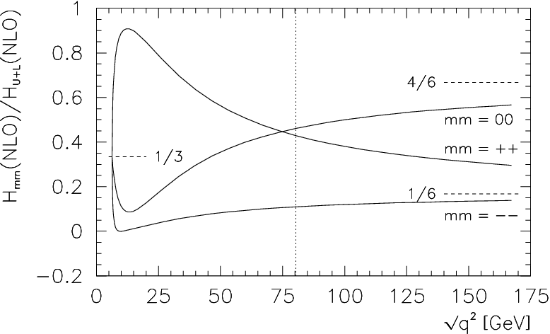
Figure 6: Energy dependence of the NLO corrections to Hm​m​(NLO)H_{mm}({\rm NLO}) (m=±,0m=\pm,0), divided by HU+L​(NLO)=H−⁣−​(NLO)+H00​(NLO)+H+⁣+​(NLO)H_{U+L}({\rm NLO})=H_{--}({\rm NLO})+H_{00}({\rm NLO})+H_{++}({\rm NLO}) for the (c​b¯)(c\bar{b}) case in the interval [mb+mc,mt−mb][m_{b}+m_{c},m_{t}-m_{b}]

In Fig. 6 we leave out the Born-term contributions and show the NLO corrections to Hm​m​(NLO)H_{mm}({\rm NLO}), divided by the sum of these. It is obvious that, at threshold, the effect of the Coulomb singularity drops out in this ratio and all three helicity structure functions contribute with a relative factor 1/31/3. On the other end of the spectrum in Fig. 6 the curves start their slow approach to the limiting values 1/61/6 (for H±⁣±H_{\pm\pm}) and 4/64/6 (for H00H_{00}).

Born mi=0m_{i}=0 Born mi≠0m_{i}\neq 0 O⁡(αs)​mi=0O(\alpha_{s})\ m_{i}=0 O⁡(αs)​mi≠0O(\alpha_{s})\ m_{i}\neq 0
W+→c​b¯W^{+}\to c\bar{b}
cfc_{f} −0.8142-0.8142 −0.8095-0.8095 −0.7348-0.7348 −0.7466-0.7466
AF​BA_{FB} −0.2280-0.2280 −0.2276-0.2276 −0.2234-0.2234 −0.2253-0.2253
cos⁡θ|max\cos\theta\,|_{\,\rm max} −0.2800-0.2800 −0.2811-0.2811 −0.3040-0.3040 −0.3018-0.3018
W+→c​s¯W^{+}\to c\bar{s}
cfc_{f} −0.8142-0.8142 −0.8138-0.8138 −0.7348-0.7348 −0.7352-0.7352
AF​BA_{FB} −0.2280-0.2280 −0.2280-0.2280 −0.2234-0.2234 −0.2235-0.2235
cos⁡θ|max\cos\theta\,|_{\,\rm max} −0.2800-0.2800 −0.2801-0.2801 −0.3040-0.3040 −0.3039-0.3039
Table 1: The measures cfc_{f}, AF​BA_{FB} and cos⁡θ|max\cos\theta\,|_{\rm\,max} for LO and NLO results at q2=mW2q^{2}=m_{W}^{2} for the cascade process t→b+W+(→cb¯,cs¯)t\to b+W^{+}(\to c\bar{b},\ c\bar{s}). Shown are massless results as well as results where the quark masses (ms=150​GeVm_{s}=150{\rm\,GeV}, mc=1.5​GeVm_{c}=1.5{\rm\,GeV} and mb=4.8​GeVm_{b}=4.8{\rm\,GeV}) are taken into account.

In Fig. 7 we plot the cos⁡θ\cos\theta distribution for W^​(θ)\widehat{W}(\theta). It is quite apparent that the distribution becomes flatter through the radiative corrections. Numerical values for the parameters cfc_{f}, AF​BA_{FB} and cos⁡θ|max\cos\theta\,|_{\,\rm max} can be found in Tab. 1. The negative value of the convexity parameter cfc_{f} means that the angular decay distribution is given by a downward-open parabola. Quark mass effects can be seen to be almost negligibly small for the W+→c​s¯W^{+}\to c\bar{s} channel.

Refer to caption
Figure 7: Normalized angular decay distribution W^​(θ)=W​(θ)/W\widehat{W}(\theta)=W(\theta)/W at LO (dashed line) and NLO (full line) for the on-shell decay t→b+W+(→cb¯)t\to b+W^{+}(\to c\bar{b}). The NLO result contains both initial-state and final-state corrections

We assume that it would be experimentally feasible to flavour-tag bottom and charm quark jets, at least for a large fraction of the corresponding top quark decays. If the hadronic flavour channel cannot be isolated, one has to take the appropriate flavour sums using the unitarity of the Kobayashi–Maskawa matrix. Furthermore, in the untagged case, the parity violating contribution proportional to cos⁡θ\cos\theta would drop out and the angular decay distribution would become symmetric in cos⁡θ\cos\theta. The resulting polar decay distribution reads

W^u​t​(cos⁡θ)=12​(W^t​(cos⁡θ)+W^t​(−cos⁡θ))\widehat{W}_{ut}(\cos\theta)=\frac{1}{2}\left(\,\widehat{W}_{t}(\cos\theta)+\widehat{W}_{t}(-\cos\theta)\,\right) (48)

where “tt” and “u​tut” stand for “flavour tagged” and “flavour untagged”.

Finite WW-width effects in top quark decays have been considered in Refs. [39, 40, 31] (see also Ref. [41]). We have recalculated the finite width correction to the total top quark width using the mass values of the present paper and find that the total width is reduced by 1.55%1.55\,\% by the finite width corrections. We also found that the longitudinal and transverse widths are reduced by 1.35%1.35\,\% and 1.99%1.99\,\%, resp., similar to the corresponding values found in Ref. [31]. Curiously enough, the respective finite width corrections are almost completely cancelled by the positive contributions of the perturbative electroweak corrections [39, 40, 31] such that these corrections taken together will affect the angular decay distributions only in a minor way.

9 The decays H→W−+W∗⁣+(→q1q¯2)H\to W^{-}+W^{\ast+}(\to q_{1}\bar{q}_{2})
and H→Z+Z∗(→qq¯)H\to Z+Z^{\ast}(\to q\bar{q})

In this section we consider quark mass and off-shell effects in the polar angle distribution of the decay W∗⁣+(↑)→q1q¯2W^{\ast+}(\uparrow)\to q_{1}\bar{q}_{2} where the off-shell W∗⁣+W^{\ast+} is produced in the Higgs decay H→W−+W∗⁣+H\to W^{-}+W^{\ast+}. We shall also briefly touch on the subject of the three-body decay H→Z+Z∗(→qq¯)H\to Z+Z^{\ast}(\to q\bar{q}). The corresponding leptonic modes have recently been observed at the LHC and are therefore adequately dubbed “Higgs discovery channels” [21, 22]. Off-shell effects in these decays will lead to additional scalar and scalar–longitudinal interference contributions in e.g. the off-shell decay W∗⁣+(↑)→q1q¯2W^{\ast+}(\uparrow)\to q_{1}\bar{q}_{2} well familiar from neutron beta decay and from the semileptonic decay Ξ0→Σ++μ−​ν¯μ\Xi^{0}\to\Sigma^{+}+\mu^{-}\bar{\nu}_{\mu} [42], or from the decay B→D(∗)+τ−​ν¯τB\to D^{(\ast)}+\tau^{-}\bar{\nu}_{\tau} [43]. The scalar and scalar–longitudinal interference contributions are quadratic in the quark masses and can thus be neglected at the scale q2=mW2q^{2}=m_{W}^{2}. However, for the off-shell decay H→W−+W∗⁣+H\to W^{-}+W^{\ast+} the scale is not set by mW2m_{W}^{2} but by the off-shellness of the W∗⁣+W^{\ast+} which extends from threshold q2=(m1+m2)2q^{2}=(m_{1}+m_{2})^{2} (maximal recoil point) to the zero recoil point at q2=(mH−mW)2q^{2}=(m_{H}-m_{W})^{2}, i.e. one has (mH=126​GeVm_{H}=126{\rm\,GeV})

(m1+m2)2≤q2≤(mH−mW)2.(m_{1}+m_{2})^{2}\leq q^{2}\leq(m_{H}-m_{W})^{2}. (49)

One will therefore have to carefully consider quark mass and W∗⁣+W^{\ast+} off-shell effects in the q2q^{2} region close to threshold.

The differential decay distribution for the decay H→W−W∗⁣+(→q1q¯2)H\to W^{-}W^{\ast\,+}(\to q_{1}\bar{q}_{2}) is given by

d​Γd​q2​d​cos⁡θ=gw41024​π3​|V12|2​|p→W|​|p→|mH2​q2​1(q2−mW2)2+mW2​ΓW2​23​Woff−shell​(θ)\frac{d\Gamma}{dq^{2}d\cos\theta}=\frac{g_{w}^{4}}{1024\pi^{3}}|V_{12}|^{2}\frac{|\vec{p}_{W}||\vec{p}|}{m_{H}^{2}\sqrt{q^{2}}}\frac{1}{(q^{2}-m_{W}^{2})^{2}+m_{W}^{2}\Gamma_{W}^{2}}\frac{2}{3}\,W_{\rm off-shell}(\theta) (50)

(gw2=8​mW2​GF/2=0.4265g_{w}^{2}=8m_{W}^{2}G_{F}/\sqrt{2}=0.4265) where the polar angle decay distribution reads

Woff−shell​(θ)=32​(−gμ​μ′+qμ​qμ′mW2)​(−gν​ν′+qν​qν′mW2)​ρμ​ν​Hμ′​ν′,W_{\rm off-shell}(\theta)=\,\frac{3}{2}\Big(-g^{\mu\mu^{\prime}}+\frac{q^{\mu}q^{\mu^{\prime}}}{m_{W}^{2}}\Big)\Big(-g^{\nu\nu^{\prime}}+\frac{q^{\nu}q^{\nu^{\prime}}}{m_{W}^{2}}\Big)\rho_{\mu\nu}H_{\mu^{\prime}\nu^{\prime}}, (51)

and where |p→W|=λ1/2​(mH2,mW2,q2)/2​mH|\vec{p}_{W}|=\lambda^{1/2}(m_{H}^{2},m_{W}^{2},q^{2})\,/2m_{H} and |p→|=q2​λ1/2​(1,μ1,μ2)/2|\vec{p}|=\sqrt{q^{2}}\lambda^{1/2}(1,\mu_{1},\mu_{2})/2 are the magnitudes of the momentum of the WW in the HH rest system and the momentum of the quarks in the W∗⁣+W^{\ast+} rest system, respectively.

We use the unitary gauge for the electroweak sector in which the numerator of the gauge boson propagator takes the unitary form written down in Eq. (51). An identical result is obtained in a general (‘t Hooft–Feynman) RξR_{\xi} gauge where one has to consider also Goldstone boson exchange. The issue of the gauge invariance of using the Breit–Wigner form for the propagator numerator has been discussed in Refs. [44, 45]. The gauge invariant complex mass scheme features such a Breit–Wigner form for the propagator denominator. In addition, complex masses have to be used in the coupling factors of the H​W​WHWW and H​Z​ZHZZ vertices (see e.g. Eq. (54)) as well as in the relation between the weak mixing angle θW\theta_{W} and the gauge boson masses. Numerically, these corrections to observable quantities amount to less than one promille and are therefore not discussed any further.

In Eq. (50) we have integrated out a trivial azimuthal angle dependence. The polarization of the W∗⁣+W^{\ast+} is encoded in the density matrix function ρμ​ν\rho_{\mu\nu} which in turn is determined from the decay H→W−​W∗⁣+H\to W^{-}W^{\ast+}. The hadron tensor Hμ​νH_{\mu\nu} contains the decay dynamics of the decay W∗⁣+→q1​q¯2W^{\ast+}\to q_{1}\bar{q}_{2} as described in Sec. 3.

One can separate the spin 1 and spin 0 parts of the propagators in Eq. (51) by writing66 6 In the analysis of Refs. [46, 47] only the spin 1 piece of the propagator is kept which is adequate for the zero lepton mass case.

(−gμ​μ′+qμ​qμ′mW2)=(−gμ​μ′+qμ​qμ′q2−qμ​qμ′q2​(1−q2mW2)).\Big(-g^{\mu\mu^{\prime}}+\frac{q^{\mu}q^{\mu^{\prime}}}{m_{W}^{2}}\Big)=\Big(-g^{\mu\mu^{\prime}}+\frac{q^{\mu}q^{\mu^{\prime}}}{q^{2}}-\frac{q^{\mu}q^{\mu^{\prime}}}{q^{2}}(1-\frac{q^{2}}{m_{W}^{2}})\Big). (52)

Note that, in the product of the two off-shell propagators in Eq. (50), the scalar–longitudinal interference term acquires an extra minus sign.

The polar angle decay distribution of a spin 1 boson decaying into a quark pair described in Sec. 3 will be augmented by the contribution of a scalar–longitudinal interference term and a scalar contribution. One has

Woff−shell​(θ)\displaystyle W_{\rm off-shell}(\theta) =\displaystyle= 32​∑m,m′=0,±ρm​m​dm​m′1​(θ)​dm​m′1​(θ)​Hm′​m′\displaystyle\frac{3}{2}\sum_{m,m^{\prime}=0,\pm}\rho_{mm}\,d^{1}_{mm^{\prime}}(\theta)\,d^{1}_{mm^{\prime}}(\theta)\,\,H_{m^{\prime}m^{\prime}} (53)
−32​(1−q2mW2)​(ρt​0​Ht​0+ρ0​t​H0​t)​cos⁡θ+32​(1−q2mW2)2​ρt​t​Ht​t.\displaystyle-\frac{3}{2}\,\Big(1-\frac{q^{2}}{m_{W}^{2}}\Big)\left(\rho_{t0}H_{t0}+\rho_{0t}H_{0t}\right)\cos\theta+\frac{3}{2}\,\Big(1-\frac{q^{2}}{m_{W}^{2}}\Big)^{2}\rho_{tt}H_{tt}.\qquad

In the next step we calculate the density matrix elements of the off-shell W∗⁣+W^{\ast+} in the decay H→W−W∗⁣+(↑)H\to W^{-}W^{\ast+}(\uparrow) where we sum over the three polarization states of the on-shell W−W^{-}. In the SM the Higgs particle couples to a pair of WW bosons via the metric tensor, i.e. the matrix element for H→W−​W+H\to W^{-}W^{+} is given by

ℳ=i​mW​gw​gμ​ν​εW−∗μ​εq∗ν,{\cal M}=im_{W}g_{w}\,g_{\mu\nu}\varepsilon^{\ast\mu}_{W^{-}}\varepsilon^{\ast\nu}_{q}, (54)

where εW−\varepsilon_{W^{-}} and εq\varepsilon_{q} denote the polarization vectors of the on-shell W−W^{-} and the off-shell W∗⁣+W^{\ast+} boson, respectively. On squaring and summing over the three spin states of the on-shell W−W^{-} one obtains the density matrix elements

ρm​m′=mW2​(−gμ​ν+pWμ​pWνmW2)​εq​μ∗​(m)​εq​ν​(m′).\rho_{mm^{\prime}}=m_{W}^{2}\left(-g^{\mu\nu}+\frac{p_{W}^{\mu}p_{W}^{\nu}}{m_{W}^{2}}\right)\varepsilon^{\ast}_{q\mu}(m)\varepsilon_{q\nu}(m^{\prime}). (55)

The square of the coupling factor gwg_{w} does not appear in Eq. (55) since we have taken the freedom to absorb gw2g_{w}^{2} in the overall factor in the rate formula (50).

We calculate the density matrix elements ρm​m′\rho_{mm^{\prime}} in the Higgs rest frame with the zz axis along the W∗⁣+W^{\ast+} momentum q=pH−pWq=p_{H}-p_{W}. Let us collect the relevant expressions for the four-momentum and the polarization vectors of the W∗⁣+W^{\ast+} boson. One has

qμ\displaystyle q^{\mu} =\displaystyle= (q0,0,0,|p→W|),q0=12​mH​(mH2+q2−mW2),εqμ​(±)=12​(0,∓1,−i,0),\displaystyle\Big(q_{0};0,0,|\vec{p}_{W}|\Big),\quad q_{0}\ =\ \frac{1}{2m_{H}}(m_{H}^{2}+q^{2}-m_{W}^{2}),\quad\varepsilon_{q}^{\mu}(\pm)\ =\ \frac{1}{\sqrt{2}}\,\Big(0;\mp 1,-i,0\Big),
εqμ​(0)\displaystyle\varepsilon_{q}^{\mu}(0) =\displaystyle= 1q2​(|p→W|,0,0,q0),εqμ​(t)=qμq2=1q2​(q0,0,0,|p→W|).\displaystyle\frac{1}{\sqrt{q^{2}}}\Big(|\vec{p}_{W}|;0,0,q_{0}\Big),\qquad\varepsilon_{q}^{\mu}(t)\ =\ \frac{q^{\mu}}{\sqrt{q^{2}}}\ =\ \frac{1}{\sqrt{q^{2}}}\Big(q_{0};0,0,|\vec{p}_{W}|\Big). (56)

The propagation of the scalar degree of freedom can be made explicit by expanding the propagator in terms of a complete set of polarization vectors (see e.g. Ref. [42, 43])

−gμ​ν+qμ​qνmW2=−∑m,m′=t,±,0εq​μ(m)εq​ν∗(m′)gm​m′-g_{\mu\nu}+\frac{q_{\mu}q_{\nu}}{m^{2}_{W}}=-\sum_{m,m^{\prime}=t,\pm,0}\varepsilon_{q\mu}(m)\varepsilon^{\ast}_{q\nu}(m^{\prime})g_{mm^{\prime}} (57)

where gm​m′=diag ​{A;−1,−1,−1}g_{mm^{\prime}}=\mbox{diag\,}\{A;-1,-1,-1\} with A=(1−q2/mW2)A=(1-q^{2}/m^{2}_{W}). The scalar degree of freedom proportional to εq​μ​(t)​εq​ν∗​(t)\varepsilon_{q\mu}(t)\varepsilon^{\ast}_{q\nu}(t) propagates from the H​W​WHWW vertex to the W​f​f¯Wf\bar{f} vertex. The scalar degree of freedom only comes into play for nonzero fermion masses.

On evaluating Eq. (55) one obtains

ρ+⁣+=ρ−⁣−\displaystyle\rho_{++}\ =\ \rho_{--} =\displaystyle= mW2,ρ00=mW2​(1+mH2q2​mW2​|p→W|2),\displaystyle m_{W}^{2},\qquad\qquad\qquad\qquad\rho_{00}\ =\ m_{W}^{2}\Big(1+\frac{m_{H}^{2}}{q^{2}m_{W}^{2}}|\vec{p}_{W}|^{2}\Big),
ρ0​t=ρt​0\displaystyle\rho_{0t}\ =\ \rho_{t0} =\displaystyle= mW2​mH​|p→W|2​mW2​q2​(mH2−mW2−q2),ρt​t=mW2​mH2q2​mW2​|p→W|2.\displaystyle m_{W}^{2}\frac{m_{H}|\vec{p}_{W}|}{2m_{W}^{2}q^{2}}\left(m_{H}^{2}-m_{W}^{2}-q^{2}\right),\qquad\rho_{tt}\ =\ m_{W}^{2}\frac{m_{H}^{2}}{q^{2}m_{W}^{2}}|\vec{p}_{W}|^{2}.\qquad (58)

At threshold (maximal recoil) when q2→(m1+m2)2q^{2}\to(m_{1}+m_{2})^{2}, and for mi→0m_{i}\to 0, the longitudinal and scalar contributions ρ00=ρt​t=ρt​0=(mH2−mW2)2/4​q2\rho_{00}=\rho_{tt}=\rho_{t0}=(m_{H}^{2}-m_{W}^{2})^{2}/4q^{2} become dominant. On the other end of the q2q^{2} spectrum (zero recoil) where |p→W|=0|\vec{p}_{W}|=0, one finds ρ+⁣+=ρ00=ρ−⁣−=mW2\rho_{++}=\rho_{00}=\rho_{--}=m_{W}^{2} and ρt​t=ρt​0=0\rho_{tt}=\rho_{t0}=0.

Since the decay H→W−​W∗⁣+H\to W^{-}W^{\ast+} is parity-conserving, the transverse density matrix elements ρ+⁣+\rho_{++} and ρ−⁣−\rho_{--} are identical to each other, i.e. one has ρ+⁣+−ρ−⁣−=0\rho_{++}-\rho_{--}=0. This means that there is no parity-violating contribution to the cos⁡θ\cos\theta coefficient in the (first) spin 1 part of Eq. (53) (see Eq. (16)). The second cos⁡θ\cos\theta contribution in Eq. (53) does not have a parity-violating origin but is a parity-odd effect. It arises from the scalar–longitudinal interference contribution with JPJ^{P} properties (0+,1−)(0^{+},1^{-}) (VV) and (0−,1+)(0^{-},1^{+}) (AA), resulting in a parity-odd contribution.

The polarized decay functions H±⁣±H_{\pm\pm} and H00H_{00} have been calculated before. The LO and NLO forms of the additional polarized decay functions Ht​tH_{tt} and Ht​0H_{t0} can be found in Sec. 2 and in Appendix D. For the convenience of the reader we list Ht​tH_{tt} and Ht​0H_{t0} together with their O⁡(μi)O(\mu_{i}) mass expansion. One has

Ht​t\displaystyle H_{tt} =\displaystyle= 4​Nc​q2​(1−μ1−μ2−λ+HS1​(αs))\displaystyle 4N_{c}q^{2}\left(1-\mu_{1}-\mu_{2}-\lambda+H^{1}_{S}(\alpha_{s})\right) (59)
=\displaystyle= 4​Nc​q2​(μ1+μ2+…+αs6​π​(18​μ1+18​μ2+12​μ1​ln⁡μ1+12​μ2​ln⁡μ2+…))\displaystyle 4N_{c}q^{2}\left(\mu_{1}+\mu_{2}+\ldots+\frac{\alpha_{s}}{6\pi}\Big(18\mu_{1}+18\mu_{2}+12\mu_{1}\ln\mu_{1}+12\mu_{2}\ln\mu_{2}+\ldots\Big)\right)\qquad

and

Ht​0\displaystyle H_{t0} =\displaystyle= H0​t= 4​Nc​q2​(−(μ1−μ2)​λ+H0​t1​(αs))\displaystyle H_{0t}\ =\ 4N_{c}q^{2}\left(-(\mu_{1}-\mu_{2}){\sqrt{\lambda}}+H^{1}_{0t}(\alpha_{s})\right) (60)
=\displaystyle= −4​Nc​q2​(μ1−μ2+…CLOSE\displaystyle-4N_{c}q^{2}\bigg(\mu_{1}-\mu_{2}+\ldots
OPEN+αs6​π​(26​μ1−14​μ2−4​π​(μ1−μ2)+12​μ1​ln⁡μ1+12​μ2​ln⁡μ2+…)).\displaystyle+\frac{\alpha_{s}}{6\pi}\Big(26\mu_{1}-14\mu_{2}-4\pi(\mu_{1}-\mu_{2})+12\mu_{1}\ln\mu_{1}+12\mu_{2}\ln\mu_{2}+\ldots\Big)\bigg).

On integrating Eq. (50) over cos⁡θ\cos\theta one obtains the differential q2q^{2} rate which is given by

d​Γd​q2\displaystyle\frac{d\Gamma}{dq^{2}} =\displaystyle= gw41024​π3​|V12|2​|p→W|​|p→|mH2​q2​1(q2−mW2)2+mW2​ΓW2\displaystyle\frac{g_{w}^{4}}{1024\pi^{3}}|V_{12}|^{2}\frac{|\vec{p}_{W}||\vec{p}\,|}{m_{H}^{2}\sqrt{q^{2}}}\frac{1}{(q^{2}-m_{W}^{2})^{2}+m_{W}^{2}\Gamma_{W}^{2}} (61)
×23​((ρ+⁣++ρ00+ρ−⁣−)​(H+⁣++H00+H−⁣−)+3​(1−q2mW2)2​ρt​t​Ht​t).\displaystyle\times\frac{2}{3}\Big((\rho_{++}+\rho_{00}+\rho_{--})(H_{++}+H_{00}+H_{--})+3(1-\frac{q^{2}}{m_{W}^{2}})^{2}\rho_{tt}H_{tt}\Big).

In the zero quark mass limit mi→0m_{i}\to 0 where H+⁣++H00+H−⁣−=8​Nc​q2H_{++}+H_{00}+H_{--}=8N_{c}q^{2} and Ht​t=0H_{tt}=0, the Born-term rate calculated from Eq. (61) can be seen to agree with the result of Refs. [48, 49] when NcN_{c} is set to one.77 7 As pointed out in Ref. [48], the corresponding result in Ref. [50] is too small by a factor of 3/43/4.

Refer to caption
Figure 8: Differential rate for the three body decay H→W−+W∗⁣+(→cb¯)H\to W^{-}+W^{\ast+}(\to c\bar{b}). The three curves correspond to (i) Born term (mi=0)(m_{i}=0) (dotted line) (ii) Born term (mi≠0)(m_{i}\neq 0) (dashed line) and (iii) O⁡(αs)O(\alpha_{s}) with (mi≠0)(m_{i}\neq 0) (full line).

In our numerical discussion we again concentrate on the mode H→W−+W∗⁣+(→cb¯)H\to W^{-}+W^{\ast+}(\to c\bar{b}) in order to highlight quark mass effects even if this mode is suppressed by |Vc​b|2=(0.041)2|V_{cb}|^{2}=(0.041)^{2}. In Fig. 8 we show the q2q^{2} dependence of the rate. Let us begin our discussion with the Born-term contributions. In the threshold region, where the longitudinal W∗⁣+W^{\ast+} dominates, the mi≠0m_{i}\neq 0 differential rate clearly shows the appropriate threshold behaviour 2​|p→|/q2=λ1/2​(1,μ1,μ2)2|\vec{p}\,|/\sqrt{q^{2}}=\lambda^{1/2}(1,\mu_{1},\mu_{2}), i.e. the differential rate vanishes at threshold. This vanishing is not seen for the mi=0m_{i}=0 curve. This can be understood by taking the mi→0m_{i}\to 0 limit of λ1/2​(1,μ1,μ2)\lambda^{1/2}(1,\mu_{1},\mu_{2}) keeping q2q^{2} small and fixed with the result λ1/2​(1,μ1,μ2)→1\lambda^{1/2}(1,\mu_{1},\mu_{2})\,\to 1. For the q2=0q^{2}=0 value of the differential mi=0m_{i}=0 rate one then obtains

d​Γd​q2|q2=0=gw41024​π3​|V12|2​Nc3​(mH2−mW2)3mH3​mW2​(mW2+ΓW2)=9.554⋅10−11​GeV−1.\frac{d\Gamma}{dq^{2}}\,\bigg|_{q^{2}=0}=\frac{g_{w}^{4}}{1024\pi^{3}}|V_{12}|^{2}\frac{N_{c}}{3}\frac{(m_{H}^{2}-m_{W}^{2})^{3}}{m_{H}^{3}m_{W}^{2}(m_{W}^{2}+\Gamma_{W}^{2})}=9.554\cdot 10^{-11}{\rm\,GeV}^{-1}. (62)

in agreement with Fig. 8. At higher values of q2q^{2} the difference between the mi=0m_{i}=0 and mi≠0m_{i}\neq 0 Born-term curves becomes smaller and smaller. The radiative corrections are largest in the threshold region. Away from the threshold region they amount to over 10%10\,\% and are thus considerably larger than what would result from the simple estimate αs/π∼3.7%\alpha_{s}/\pi\sim 3.7\,\%. We mention that the radiative corrections to the LO mi=0m_{i}=0 curve in Fig. 8 is simply given by multiplying the LO result by (1+αs/π)(1+\alpha_{s}/\pi).

Fig. 8 also shows that the O⁡(αs)O(\alpha_{s}) mi≠0m_{i}\neq 0 rate does not go to zero at threshold. This can be traced to the presence of the NLO chromodynamic Coulomb singularity at threshold. The Coulomb singularity proportional to λ−1/2\lambda^{-1/2} (see Eq. (C4)) is cancelled by the overall rate factor |p→|=q2​λ1/2/2|\vec{p}\,|=\sqrt{q^{2}}\lambda^{1/2}/2 resulting in a finite contribution at threshold proportional to αs\alpha_{s}. One can estimate the finite threshold value of the O⁡(αs)O(\alpha_{s}) rate by neglecting terms of O⁡(q2/mW2)O(q^{2}/m_{W}^{2}) in Eq. (61) whence one can express the finite threshold value in terms of the LO mi=0m_{i}=0 contribution in Eq. (62). One then obtains

d​Γd​q2|thresh≈αs​32​π3​μ1​μ2​d​Γd​q2|q2=0.\frac{d\Gamma}{dq^{2}}\,\bigg|_{\rm thresh}\approx\alpha_{s}\,\frac{32\pi}{3}\,\mu_{1}\mu_{2}\,\frac{d\Gamma}{dq^{2}}\,\bigg|_{q^{2}=0}. (63)

Using αs​(q2=(4.8+1.5)2​GeV2)=0.165\alpha_{s}(q^{2}=(4.8+1.5)^{2}{\rm\,GeV}^{2})=0.165, one obtains approximate agreement with Fig. 8. As has been emphasized before, perturbation theory cannot be trusted in the threshold region and therefore the treatment of the decay W∗⁣+→c​b¯W^{\ast+}\to c\bar{b} requires a nonperturbative treatment including a resummation of the chromodynamic Coulomb singularity. The above exercise leading to Eq. (63) merely serves to check on the consistency of our calculation.

In Fig. 9 we show a plot of the q2q^{2} dependence of the convexity parameter. The convexity parameter is obtained from Eq. (61) by replacing (ρ+⁣++ρ00+ρ−⁣−)​(H+⁣++H00+H−⁣−)(\rho_{++}+\rho_{00}+\rho_{--})(H_{++}+H_{00}+H_{--}) by 3/4​(ρ+⁣+−2​ρ00+ρ−⁣−)​(H+⁣+−2​H00+H−⁣−)3/4(\rho_{++}-2\rho_{00}+\rho_{--})(H_{++}-2H_{00}+H_{--}), setting the scalar contribution to zero, and then dividing by the differential rate (61). At threshold and at zero recoil the convexity parameter can be seen to go to zero at both ends of the q2q^{2} spectrum because one has H+⁣+−2​H00+H−⁣−→0H_{++}-2H_{00}+H_{--}\to 0 at threshold and ρ+⁣+−2​ρ00+ρ−⁣−→0\rho_{++}-2\rho_{00}+\rho_{--}\to 0 at zero recoil.

An interesting exercise is to calculate the LO convexity parameter in the threshold region. Neglecting terms of O⁡(q2/mZ2)O(q^{2}/m_{Z}^{2}), as before, one obtains

cf∼−32​(λ3−3​μ1−3​μ2−2​λ).c_{f}\sim-\frac{3}{2}\,\left(\frac{\lambda}{3-3\mu_{1}-3\mu_{2}-2\lambda}\right). (64)

The expression (64) has the correct threshold behaviour. Keeping q2q^{2} fixed (and small), and taking the limit mi→0m_{i}\to 0 one has μi→0\mu_{i}\to 0, λ→1\lambda\to 1 and one obtains cf=−3/2c_{f}=-3/2 in agreement with Fig. 9.

Refer to caption
Figure 9: Convexity parameter cf​(q2)c_{f}(q^{2}) as a function of q2q^{2}. Labelling of curves as in Fig. 8
Refer to caption
Figure 10: Differential rate d​ΓU/d​q2d\Gamma_{U}/d{q^{2}}. Labelling of curves as in Fig. 8
Refer to caption
Figure 11: Differential rate d​ΓL/d​q2d\Gamma_{L}/d{q^{2}}. Labelling of curves as in Fig. 8
Refer to caption
Figure 12: Differential rate d​ΓS/d​q2d\Gamma_{S}/d{q^{2}}. Labelling of curves as in Fig. 8

In Figs. 10–12 we decompose the total differential rate d​Γ/d​q2d\Gamma/dq^{2} in terms of the three partial unpolarized transverse (UU), longitudinal (LL) and scalar (SS) contributions d​ΓU/d​q2d\Gamma_{U}/dq^{2}, d​ΓL/d​q2d\Gamma_{L}/dq^{2} and d​ΓS/d​q2d\Gamma_{S}/dq^{2}, where the three partial rates are defined by the contributions of the density matrix elements ρ+⁣++ρ−⁣−\rho_{++}+\rho_{--}, ρ00\rho_{00} and ρt​t\rho_{tt}, respectively. The total rate is then given by d​Γ/d​q2=d​ΓU/d​q2+d​ΓL/d​q2+d​ΓS/d​q2d\Gamma/dq^{2}=d\Gamma_{U}/dq^{2}+d\Gamma_{L}/dq^{2}+d\Gamma_{S}/dq^{2}.

Fig. 10 shows that the transverse rate is weighted toward higher q2q^{2} values, whereas the longitudinal rate is more evenly distributed (Fig. 11). The scalar rate is considerably smaller and shows a peak close to threshold (Fig. 12). The peak value is strongly enhanced by the radiative corrections. The radiative corrections to the transverse rate are small. The radiative corrections to the longitudinal rate can be seen to be quite pronounced close to threshold which, in part, is due to the increase of αs\alpha_{s} due to running.

Born mi=0m_{i}=0 Born mi≠0m_{i}\neq 0 O⁡(αs)​mi=0O(\alpha_{s})\ m_{i}=0 O⁡(αs)​mi≠0O(\alpha_{s})\ m_{i}\neq 0
W∗⁣+→c​b¯W^{\ast+}\to c\bar{b}
Γ\Gamma 2.43⋅10−72.43\cdot 10^{-7} 2.30⋅10−72.30\cdot 10^{-7} 2.55⋅10−72.55\cdot 10^{-7} 2.45⋅10−72.45\cdot 10^{-7}
ΓU\Gamma_{U} 9.79⋅10−89.79\cdot 10^{-8} 9.40⋅10−89.40\cdot 10^{-8} 1.02⋅10−71.02\cdot 10^{-7} 9.98⋅10−89.98\cdot 10^{-8}
ΓL\Gamma_{L} 1.45⋅10−71.45\cdot 10^{-7} 1.29⋅10−71.29\cdot 10^{-7} 1.52⋅10−71.52\cdot 10^{-7} 1.39⋅10−71.39\cdot 10^{-7}
ΓS\Gamma_{S} 00 6.67⋅10−96.67\cdot 10^{-9} 00 6.81⋅10−96.81\cdot 10^{-9}
AF​BA_{FB} 00 0.01940.0194 00 0.01900.0190
W∗⁣+→c​s¯W^{\ast+}\to c\bar{s}
Γ\Gamma 1.37⋅10−41.37\cdot 10^{-4} 1.36⋅10−41.36\cdot 10^{-4} 1.44⋅10−41.44\cdot 10^{-4} 1.43⋅10−41.43\cdot 10^{-4}
ΓU\Gamma_{U} 5.52⋅10−55.52\cdot 10^{-5} 5.50⋅10−55.50\cdot 10^{-5} 5.77⋅10−55.77\cdot 10^{-5} 5.76⋅10−55.76\cdot 10^{-5}
ΓL\Gamma_{L} 8.19⋅10−58.19\cdot 10^{-5} 8.06⋅10−58.06\cdot 10^{-5} 8.58⋅10−58.58\cdot 10^{-5} 8.49⋅10−58.49\cdot 10^{-5}
ΓS\Gamma_{S} 00 7.46⋅10−77.46\cdot 10^{-7} 00 6.53⋅10−76.53\cdot 10^{-7}
AF​BA_{FB} 00 −0.00433-0.00433 00 −0.00339-0.00339
Z∗→b​b¯Z^{\ast}\to b\bar{b}
Γ\Gamma 7.47⋅10−67.47\cdot 10^{-6} 5.98⋅10−65.98\cdot 10^{-6} 7.82⋅10−67.82\cdot 10^{-6} 6.68⋅10−66.68\cdot 10^{-6}
ΓU\Gamma_{U} 3.03⋅10−63.03\cdot 10^{-6} 2.51⋅10−62.51\cdot 10^{-6} 3.16⋅10−63.16\cdot 10^{-6} 2.77⋅10−62.77\cdot 10^{-6}
ΓL\Gamma_{L} 4.44⋅10−64.44\cdot 10^{-6} 2.95⋅10−62.95\cdot 10^{-6} 4.66⋅10−64.66\cdot 10^{-6} 3.34⋅10−63.34\cdot 10^{-6}
ΓS\Gamma_{S} 00 5.11⋅10−75.11\cdot 10^{-7} 00 5.72⋅10−75.72\cdot 10^{-7}
AF​BA_{FB} 00 00 00 0.0005540.000554
Z∗→c​c¯Z^{\ast}\to c\bar{c}
Γ\Gamma 5.79⋅10−65.79\cdot 10^{-6} 5.65⋅10−65.65\cdot 10^{-6} 6.06⋅10−66.06\cdot 10^{-6} 5.99⋅10−65.99\cdot 10^{-6}
ΓU\Gamma_{U} 2.35⋅10−62.35\cdot 10^{-6} 2.29⋅10−62.29\cdot 10^{-6} 2.45⋅10−62.45\cdot 10^{-6} 2.42⋅10−62.42\cdot 10^{-6}
ΓL\Gamma_{L} 3.45⋅10−63.45\cdot 10^{-6} 3.20⋅10−63.20\cdot 10^{-6} 3.61⋅10−63.61\cdot 10^{-6} 3.42⋅10−63.42\cdot 10^{-6}
ΓS\Gamma_{S} 00 1.55⋅10−71.55\cdot 10^{-7} 00 1.42⋅10−71.42\cdot 10^{-7}
AF​BA_{FB} 00 00 00 0.0004240.000424
Table 2: Integrated rates Γ,ΓU,ΓL,ΓS\Gamma,\Gamma_{U},\Gamma_{L},\Gamma_{S} and forward–backward asymmetry AF​BA_{FB} for H→W−+W∗⁣+(→cb¯)H\to W^{-}+W^{\ast+}(\to c\bar{b}), H→W−+W∗⁣+(→cc¯)H\to W^{-}+W^{\ast+}(\to c\bar{c}), H→Z+Z∗(→bb¯)H\to Z+Z^{\ast}(\to b\bar{b}) and H→Z+Z∗(→cc¯)H\to Z+Z^{\ast}(\to c\bar{c}). All entries are given in units of GeV{\rm\,GeV} except for AF​BA_{FB}.

In Tab. 2 we present our numerical results for the integrated total rate and the integrated partial rates for W+→c​b¯W^{+}\to c\bar{b}. One can see that the integrated longitudinal rate ΓL\Gamma_{L} slightly dominates over the integrated transverse rate ΓU\Gamma_{U}. The scalar rate ΓS\Gamma_{S} is quite small and contributes to the total rate at the 2.9%2.9\,\% level. The LO total rate is reduced by 5.8%5.8\,\% through mass effects where the biggest reduction comes from the longitudinal rate (11.7%11.7\,\%). Radiative corrections increase the LO rates by 6.2%−7.8%6.2\,\%-7.8\,\% except for the scalar rate which is increased only by 2.1%2.1\,\%. We also list the value of the forward–backward asymmetry AF​BA_{FB} which, as has been discussed before, is a parity-odd effect contributed to by the parity-conserving scalar–longitudinal interference term. The forward–backward asymmetry is positive (see Eqs. (53) and (60)) and receives its main contribution from the region close to threshold. AF​BA_{FB} is of the same order of magnitude as ΓS/ΓL\Gamma_{S}/\Gamma_{L}. For comparison, in Tab. 2 we also include results for the process W+→c​s¯W^{+}\to c\bar{s} (|Vc​s|=0.97345±00016|V_{cs}|=0.97345\pm 00016 [27]).

Quark mass effects can be expected to play a larger role in e.g. the decay H→Z+Z∗(→bb¯)H\to Z+Z^{\ast}(\to b\bar{b}). First, the b​b¯b\bar{b} threshold is higher than the c​b¯c\bar{b} threshold, and second, the phase space is reduced due to the larger mass of the ZZ boson, i.e. the physical q2q^{2} range becomes smaller. An extra bonus is the fact that the decay Z∗→b​b¯Z^{\ast}\to b\bar{b} is not CKM suppressed. For the differential decay distribution one obtains (sin2⁡θW=0.23188\sin^{2}\theta_{W}=0.23188)

d​Γd​q2\displaystyle\frac{d\Gamma}{dq^{2}} =\displaystyle= 12​gw41024​π3​1cos4⁡θW​|p→Z|​|p→|mH2​q2​1(q2−mZ2)2+mZ2​ΓZ2\displaystyle\frac{1}{2}\,\frac{g_{w}^{4}}{1024\pi^{3}}\frac{1}{\cos^{4}\theta_{W}}\frac{|\vec{p}_{Z}||\vec{p}\,|}{m_{H}^{2}\sqrt{q^{2}}}\frac{1}{(q^{2}-m_{Z}^{2})^{2}+m_{Z}^{2}\Gamma_{Z}^{2}} (65)
×23​((ρ+⁣++ρ00+ρ−⁣−)​12​(vf2​HU+LV​V+af2​HU+LA​A)CLOSE\displaystyle\times\frac{2}{3}\Big((\rho_{++}+\rho_{00}+\rho_{--})\frac{1}{2}(v_{f}^{2}H^{VV}_{U+L}+a_{f}^{2}H^{AA}_{U+L})
OPEN+3​(1−q2mZ2)2​ρt​t​(vf2​Ht​tV​V+af2​Ht​tA​A)),\displaystyle\qquad\qquad+3(1-\frac{q^{2}}{m_{Z}^{2}})^{2}\,\rho_{tt}(v_{f}^{2}H^{VV}_{tt}+a_{f}^{2}H^{AA}_{tt})\Big),

where the gauge boson momentum now is |p→Z|=λ⁡(mH2,mZ2,q2)/2​mH|\vec{p}_{Z}|=\sqrt{\lambda(m_{H}^{2},m_{Z}^{2},q^{2})}\,/2m_{H}, and p→W,mW\vec{p}_{W},m_{W} are replaced by p→Z,mZ\vec{p}_{Z},m_{Z} in the expressions for ρm​m′\rho_{mm^{\prime}} in Eq. (58). The electroweak coupling coefficients are given by

vf\displaystyle v_{f} =\displaystyle= 1−83​sin2⁡θW,af=1foru,c,t\displaystyle 1-\frac{8}{3}\sin^{2}\theta_{W},\qquad a_{f}=1\qquad\mbox{for}\quad u,c,t
vf\displaystyle v_{f} =\displaystyle= −1+43​sin2⁡θW,af=−1ford,s,b.\displaystyle-1+\frac{4}{3}\sin^{2}\theta_{W},\qquad a_{f}=-1\qquad\mbox{for}\quad d,s,b. (66)

In Fig. 13 we provide a plot of the differential q2q^{2} rate for H→Z+Z∗(→bb¯)H\to Z+Z^{\ast}(\to b\bar{b}) where we use mZ=91.1876±0.0021​GeVm_{Z}=91.1876\pm 0.0021{\rm\,GeV}, ΓZ=2.4952±0.0023​GeV\Gamma_{Z}=2.4952\pm 0.0023{\rm\,GeV} [27]. Again the differential LO rate shows the appropriate threshold behaviour for mb≠0m_{b}\neq 0, i.e. the differential rate vanishes at threshold q2=4​mb2q^{2}=4m_{b}^{2}.

The corresponding mb=0m_{b}=0 LO rate shows no apparent vanishing at threshold for the same reason as in the corresponding H→W−​W∗⁣+H\to W^{-}W^{\ast+} case. The differential rate at q2=0q^{2}=0 and for mb=0m_{b}=0 is given by

d​Γd​q2|q2=0=12​gw41024​π3​1cos4⁡θW​Nc3​(mH2−mZ2)3mH3​mZ2​(mZ2+ΓZ2)​12​vf2+af22=0.56⋅10−8​GeV−1.\frac{d\Gamma}{dq^{2}}\,\bigg|_{q^{2}=0}=\frac{1}{2}\,\frac{g_{w}^{4}}{1024\pi^{3}}\frac{1}{\cos^{4}\theta_{W}}\frac{N_{c}}{3}\frac{(m_{H}^{2}-m_{Z}^{2})^{3}}{m_{H}^{3}m_{Z}^{2}(m_{Z}^{2}+\Gamma_{Z}^{2})}\frac{1}{2}\frac{v_{f}^{2}+a_{f}^{2}}{2}=0.56\cdot 10^{-8}{\rm\,GeV}^{-1}. (67)

in agreement with Fig. 13.

Refer to caption
Figure 13: Differential rate for the three body decay H→Z+Z∗(→b+b¯)H\to Z+Z^{\ast}(\to b+\bar{b}). Labelling of curves as in Fig. 8.

As Fig. 13 shows, the NLO rate does not go to zero at threshold. As in the charged current case this can be traced to the presence of the NLO chromodynamic Coulomb singularity at threshold. One can estimate the finite threshold value of the O⁡(αs)O(\alpha_{s}) rate by neglecting terms of O⁡(q2/mZ2)O(q^{2}/m_{Z}^{2}) in Eq. (65) whence one can express the finite threshold value in terms of the LO mb=0m_{b}=0 contribution in Eq. (67). One then obtains

d​Γd​q2|thresh≈αs​(vf2+af2)(vf2+3​af2)​16​π3​μ2​d​Γd​q2|q2=0.\frac{d\Gamma}{dq^{2}}\,\bigg|_{\rm thresh}\approx\,\alpha_{s}\,\frac{(v_{f}^{2}+a_{f}^{2})}{(v_{f}^{2}+3a_{f}^{2})}\frac{16\pi}{3}\mu^{2}\,\frac{d\Gamma}{dq^{2}}\,\bigg|_{q^{2}=0}. (68)

Note that the contribution proportional to 3​af23a_{f}^{2} results from the scalar contribution in Eq. (65). By a visual inspection of Fig. 13, the approximation can be seen to be quite good. Similar to the calculation leading up to Eq. (64) one can calculate the LO convexity parameter in the threshold region. Neglecting again terms of O⁡(q2/mZ2)O(q^{2}/m_{Z}^{2}) one finds

cf=−32​(1−4​μ1+2​μ)c_{f}=-\frac{3}{2}\left(\frac{1-4\mu}{1+2\mu}\right) (69)

which is just the limiting case of Eq. (64) for μ1=μ2:=μ\mu_{1}=\mu_{2}:=\mu. Curiously the intricate dependence on the electroweak coupling parameters cfc_{f} and afa_{f} has dropped out when taking the ratio. In the mass-zero case and at q2=0q^{2}=0 one has exactly cf=−3/2c_{f}=-3/2.

Refer to caption
Figure 14: q2q^{2} dependence of the convexity parameter cf​(q2)c_{f}(q^{2}) for H→Z+Z∗(→b+b¯)H\to Z+Z^{\ast}(\to b+\bar{b}). Labelling of curves as in Fig. 8

In Fig. 14 we show a plot of the q2q^{2} dependence of the convexity parameter cfc_{f}. In the threshold region the convexity parameter behaves very differently for mb=0m_{b}=0 and mb≠0m_{b}\neq 0 (the radiative corrections are quite small). This implies that the polar angle distributions are very different for the two cases. In order to illustrate this effect we choose q2=150​GeV2q^{2}=150{\rm\,GeV}^{2} and, in Fig. 15, plot the corresponding cos⁡θ\cos\theta distribution. At this value of q2q^{2} one is well outside of the nonperturbative threshold region. Since the convexity parameter is negative (see Eq. (69)), one has a downward open parabola. Mass effects can be seen to be crucial for the correct description of the m≠0m\neq 0 angular decay distribution which is much flatter than the m=0m=0 distribution. The three curves correspond to convexity parameters of cf=−1.154c_{f}=-1.154 (LO; mb=0m_{b}=0), cf=−0.388c_{f}=-0.388 (LO) and cf=−0.407c_{f}=-0.407 (NLO).

Refer to caption
Figure 15: Polar angle distribution for Z∗(→b+b¯)Z^{\ast}(\to b+\bar{b}) at q2=150​GeV2q^{2}=150{\rm\,GeV}^{2}. Labelling of curves as in Fig. 8

In Table 2 we have listed numerical values for the various integrated partial rates and for the asymmetry parameter AF​BA_{FB} for both Z∗→b​b¯Z^{\ast}\to b\bar{b} and for Z∗→c​c¯Z^{\ast}\to c\bar{c}. Quark mass effects and scalar contributions can be seen to be quite large in particular for the b​b¯b\bar{b} case. In the b​b¯b\bar{b} case, mass effects decrease the LO rate by 20.1%20.1\,\% where most of this reduction comes from ΓL\Gamma_{L}. The scalar contribution amounts to 8.6%8.6\,\% of the total contribution. The radiative corrections increase all four rates by O⁡(10%)O(10\,\%). The scalar–longitudinal interference contribution sets in only at O⁡(αs)O(\alpha_{s}) since the Born-term contribution to H0​tH_{0t} vanishes, i.e. the forward–backward asymmetry is proportional to αs\alpha_{s} and therefore small. This is borne out by the tiny numerical value of AF​BA_{FB} listed in Table 2. The numbers in Table 2 for the c​c¯c\bar{c} case follow a similar pattern, though quark mass and off-shell effects are smaller.

In this section we have assumed one gauge boson to be on-shell and the other opposite-side gauge boson to be off-shell. The on-shell approximation can be dropped by also taking the on-shell gauge boson off its mass shell using, again, a Breit–Wigner form for the propagator. We find upward corrections to the rate of 5.2%5.2\,\% for H→W​WH\to WW and 19.9%19.9\,\% for H→Z​ZH\to ZZ.

In the present calculation we have used a factorized form for the opposite-side fermion pair decays which is only justified when one does not have identical fermions in the final state. If one has identical fermions in the final state as in H→Z∗Z∗(→fff¯f¯)H\to Z^{\ast}Z^{\ast}(\to ff\bar{f}\bar{f}), there will be interference effects involving the pairs of identical fermions. In order to account for such interference effects, a full-fledged calculation of H→Z∗​Z∗H\to Z^{*}Z^{*} with subsequent four-body decays is required, as has been done in Refs. [34, 35]. As shown in Ref. [51], these interference effects can lead to a substantial reduction in rate. For example, for a 126​GeV126{\rm\,GeV} Higgs boson interference effects reduce the branching ratio of H→e​e​μ​μH\to ee\mu\mu by 45%45\,\% when going to the decay H→e​e​e​eH\to eeee.

10 Summary and Conclusions

We have calculated the NLO QCD corrections to the polarized decay functions in the decay of an off-shell and on-shell polarized W+W^{+} gauge boson into massive quark–antiquark pairs W+(↑)→q1q¯2W^{+}(\uparrow)\to q_{1}\,\bar{q}_{2}, keeping the quark masses finite. Using these NLO results for the decay process as well as previous results on the NLO corrections to the production process t→b+W+t\to b+W^{+} we have studied the NLO corrections to the polar angle decay distribution in the cascade decay t→b+W+t\to b+W^{+} followed by W+→q1​q¯2W^{+}\rightarrow q_{1}\,\bar{q}_{2}. We have found that the NLO final-state corrections to the decay distribution are somewhat larger than the NLO initial state corrections. Altogether we find that the NLO corrections lead to a flatter angular decay distribution W⁡(θ)W(\theta).

The decay analysis was done in the W+W^{+} rest frame which has the maximal sensitivity to W+W^{+} polarization effects. Polarization effects of the W+W^{+} boson will be visible also in other reference frames such as the laboratory frame. It is therefore always important to retain W+W^{+} polarization effects in radiative correction calculations (see e.g. Refs. [34, 35, 52, 53, 54, 55]).

We have presented our results in a general form involving the spin 0 and spin 1 pieces of the (V​V)(VV), (A​A)(AA), (V​A)(VA) and (A​V)(AV) current contributions separately. Our results can thus also be applied to on-shell ZZ decays and off-shell Z∗Z^{\ast} decays (as in Sec. 9) and also to extensions of the SM.

In this paper we have discussed the decays W+→q1​q¯2W^{+}\to q_{1}\,\bar{q}_{2} of positively charged W+W^{+} bosons. The corresponding results for negatively charged bosons W−→q¯1​q2W^{-}\to\bar{q}_{1}\,q_{2} can be obtained from the CP invariance of the interaction. One finds [14]

Hm​m(W−→q¯1q2;μ1,μ2;z′∥q2)=Hm​m(W+→q1q¯2;μ2,μ1;z′∥q1).H_{mm}(W^{-}\to\bar{q}_{1}q_{2};\mu_{1},\mu_{2};z^{\prime}\parallel q_{2})=H_{mm}(W^{+}\to q_{1}\bar{q}_{2};\mu_{2},\mu_{1};z^{\prime}\parallel q_{1}). (70)

From the experimental point of view, the leptonic decay of the WW boson is the most interesting one. In a sequel to this paper we shall calculate the corresponding NLO electroweak corrections to the decay W+(↑)→ℓ+νℓW^{+}(\uparrow)\to\ell^{+}\,\nu_{\ell}.

As a further example of much topical interest we have discussed the Higgs decay modes H→W−+W∗⁣+(→cb¯,cs¯)H\to W^{-}+W^{\ast+}(\to c\bar{b},c\bar{s}) and H→Z+Z∗(→bb¯,cc¯)H\to Z+Z^{\ast}(\to b\bar{b},\,c\bar{c}) involving the off-shell W∗⁣+W^{\ast+} and Z∗Z^{\ast} bosons. We find that quark-mass effects and scalar contributions affect the rate and the angular decay distributions in these decays in a non-negligible way especially in the vicinity of the threshold region. Quark mass effects are also non-negligible for the overall rate. For example, nonzero quark masses induce a scalar contribution to the rate which makes up 8.6%8.6\,\% of the total rate for H→Z+Z∗(→bb¯)H\to Z+Z^{\ast}(\to b\bar{b}).

It would be worthwhile to exploit the knowledge about charged and neutral current spectral functions in the heavy quark sector which has been accumulating over the last few decades for a precision analysis of the rates of the decays H→W−+W∗⁣+(→bc¯)H\to W^{-}+W^{\ast+}(\to b\bar{c}) and H→Z+Z∗(→bb¯,cc¯)H\to Z+Z^{\ast}(\to b\bar{b},\,c\bar{c}).

Acknowledgements

This work was supported by the Estonian target financed project No. 0180056s09, and by the Estonian Science Foundation under grant No. 8769. J.G.K. would like to acknowledge useful discussions with B. Jäger and K. Schilcher. S.G. acknowledges the support by the Deutsche Forschungsgemeinschaft (DFG) under Grant No. 436 EST 17/1/06 and by the Forschungszentrum of the Johannes-Gutenberg-Universität Mainz “Elementarkräfte und Mathematische Grundlagen (EMG)”.

Appendix A Decay rate terms

In this appendix we present analytical expressions for the polarized decay functions introduced in the main text. For the tree-graph contributions we define logarithmic decay rate terms

ℓ1=ln⁡(1+μ1−μ2+λ1+μ1−μ2−λ),\displaystyle\ell_{1}=\ln\left(\frac{1+\mu_{1}-\mu_{2}+{\sqrt{\lambda}}}{1+\mu_{1}-\mu_{2}-{\sqrt{\lambda}}}\right), ℓ2=ln⁡(1−μ1+μ2+λ1−μ1+μ2−λ),\displaystyle\ell_{2}=\ln\left(\frac{1-\mu_{1}+\mu_{2}+{\sqrt{\lambda}}}{1-\mu_{1}+\mu_{2}-{\sqrt{\lambda}}}\right),
ℓ0=ln⁡((1−μ1)2μ2),\displaystyle\ell_{0}=\ln\left(\frac{(1-\sqrt{\mu_{1}})^{2}}{\mu_{2}}\right), ℓ4=ln⁡((1+μ1)2−μ2μ1)\displaystyle\ell_{4}=\ln\left(\frac{(1+\sqrt{\mu_{1}})^{2}-\mu_{2}}{\sqrt{\mu_{1}}}\right)\qquad (A1)

and the linear combination ℓ3=ℓ1+ℓ2\ell_{3}=\ell_{1}+\ell_{2}. One further has dilogarithmic decay rate terms given by

Izℓ​(0)\displaystyle I^{\ell}_{z}(0)\!\!\! =\displaystyle= Li2​(−z+)−Li2​(−z−)+Li2​(z+−μ1μ1​z+−1)−Li2​(μ1​z+−1z+−μ1),\displaystyle\!\!\!{\rm Li}_{2}(-z_{+})-{\rm Li}_{2}(-z_{-})+{\rm Li}_{2}\left(\frac{z_{+}-\sqrt{\mu_{1}}}{\sqrt{\mu_{1}}z_{+}-1}\right)-{\rm Li}_{2}\left(\frac{\sqrt{\mu_{1}}z_{+}-1}{z_{+}-\sqrt{\mu_{1}}}\right), (A2)
Szℓ​(0)\displaystyle S^{\ell}_{z}(0)\!\!\! =\displaystyle= Li2​(1−μ1−μ2−λ1−μ1−μ2+λ)+Li2​(1−μ1+μ2−λ1−μ1+μ2+λ)+Li2​(1+μ1−μ2−λ1+μ1−μ2+λ)\displaystyle\!\!\!{\rm Li}_{2}\left(\frac{1-\mu_{1}-\mu_{2}-{\sqrt{\lambda}}}{1-\mu_{1}-\mu_{2}+{\sqrt{\lambda}}}\right)+{\rm Li}_{2}\left(\frac{1-\mu_{1}+\mu_{2}-{\sqrt{\lambda}}}{1-\mu_{1}+\mu_{2}+{\sqrt{\lambda}}}\right)+{\rm Li}_{2}\left(\frac{1+\mu_{1}-\mu_{2}-{\sqrt{\lambda}}}{1+\mu_{1}-\mu_{2}+{\sqrt{\lambda}}}\right) (A3)
−π22+12​ln2⁡(1−μ1−μ2−λ1−μ1−μ2+λ)+ln⁡(λ2​μ1​μ2)​ln⁡(1−μ1−μ2−λ1−μ1−μ2+λ)\displaystyle-\frac{\pi^{2}}{2}+\frac{1}{2}\ln^{2}\left(\frac{1-\mu_{1}-\mu_{2}-{\sqrt{\lambda}}}{1-\mu_{1}-\mu_{2}+{\sqrt{\lambda}}}\right)+\ln\left(\frac{\lambda}{2\mu_{1}\mu_{2}}\right)\ln\left(\frac{1-\mu_{1}-\mu_{2}-{\sqrt{\lambda}}}{1-\mu_{1}-\mu_{2}+{\sqrt{\lambda}}}\right)
+2​ln⁡(2​μ1)​ln⁡(2​μ2)−2​ln⁡(1−μ1+μ2+λ)​ln⁡(1+μ1−μ2+λ),\displaystyle+2\ln(2\sqrt{\mu_{1}})\ln(2\sqrt{\mu_{2}})-2\ln(1-\mu_{1}+\mu_{2}+{\sqrt{\lambda}})\ln(1+\mu_{1}-\mu_{2}+{\sqrt{\lambda}}),
I1ℓ​(0)\displaystyle I^{\ell}_{1}(0)\!\!\! =\displaystyle= Li2​(μ1)−Li2​(μ1​z+)−Li2​(μ1​z−)−π26\displaystyle\!\!\!{\rm Li}_{2}(\mu_{1})-{\rm Li}_{2}(\sqrt{\mu_{1}}z_{+})-{\rm Li}_{2}(\sqrt{\mu_{1}}z_{-})-\frac{\pi^{2}}{6} (A4)
+12​Li2​((z−−μ1)2(1−μ1​z−)2)+12​Li2​(z−2)−2​L​i2​(μ1​(μ1−z−)1−μ1​z−)\displaystyle+\frac{1}{2}{\rm Li}_{2}\left(\frac{(z_{-}-\sqrt{\mu_{1}})^{2}}{(1-\sqrt{\mu_{1}}z_{-})^{2}}\right)+\frac{1}{2}{\rm Li}_{2}(z_{-}^{2})-2{\rm Li}_{2}\left(\frac{\sqrt{\mu_{1}}(\sqrt{\mu_{1}}-z_{-})}{1-\sqrt{\mu_{1}}z_{-}}\right)
+ln⁡(1−z−21−μ1)​ln⁡(z−−μ11−μ1​z−)+ln⁡z−​ln⁡(z+−z−),\displaystyle+\ln\left(\frac{1-z_{-}^{2}}{1-\mu_{1}}\right)\ln\left(\frac{z_{-}-\sqrt{\mu_{1}}}{1-\sqrt{\mu_{1}}z_{-}}\right)+\ln z_{-}\ln(z_{+}-z_{-}),
S1ℓ​(0)\displaystyle S^{\ell}_{1}(0)\!\!\! =\displaystyle= Li2​(z−)−Li2​(−z−)−π24+ln⁡z−​ln⁡(1−z−1+z−)\displaystyle\!\!\!{\rm Li}_{2}(z_{-})-{\rm Li}_{2}(-z_{-})-\frac{\pi^{2}}{4}+\ln z_{-}\ln\left(\frac{1-z_{-}}{1+z_{-}}\right) (A5)
−Li2​((1+μ1)​(1−z−)(1−μ1)​(1+z−))+Li2​(−(1+μ1)​(1−z−)(1−μ1)​(1+z−)),\displaystyle-{\rm Li}_{2}\left(\frac{(1+\sqrt{\mu_{1}})(1-z_{-})}{(1-\sqrt{\mu_{1}})(1+z_{-})}\right)+{\rm Li}_{2}\left(-\frac{(1+\sqrt{\mu_{1}})(1-z_{-})}{(1-\sqrt{\mu_{1}})(1+z_{-})}\right),
Iℓ​(0)\displaystyle I^{\ell}(0)\!\!\! =\displaystyle= Li2​(μ1​z+)+Li2​(μ1​z−)−2​L​i2​(μ1)+ln2⁡z−=Sℓ​(0)\displaystyle\!\!\!{\rm Li}_{2}(\sqrt{\mu_{1}}z_{+})+{\rm Li}_{2}(\sqrt{\mu_{1}}z_{-})-2{\rm Li}_{2}(\sqrt{\mu_{1}})+\ln^{2}z_{-}\ =\ S^{\ell}(0) (A6)

where

z+=12​μ1​(1+μ1−μ2+λ)=z−−1.z_{+}=\frac{1}{2\sqrt{\mu_{1}}}\left(1+\mu_{1}-\mu_{2}+{\sqrt{\lambda}}\right)=z_{-}^{-1}\,. (A7)

The decay rate terms originating from the loop corrections read

ℓA\displaystyle\ell_{A} =\displaystyle= 2​ln⁡λ−3​ln⁡μ1​μ2,\displaystyle 2\ln\lambda-3\ln\sqrt{\mu_{1}\mu_{2}}, (A8)
ℓB\displaystyle\ell_{B} =\displaystyle= ln⁡(μ1μ2),\displaystyle\ln\left(\frac{\mu_{1}}{\mu_{2}}\right), (A9)
tA\displaystyle t_{A} =\displaystyle= (ℓA−ln⁡(1−(μ1−μ2)2))​ℓ3\displaystyle\left(\ell_{A}-\ln\left(1-(\sqrt{\mu_{1}}-\sqrt{\mu_{2}})^{2}\right)\right)\ell_{3} (A10)
+Li2​(1−α+)−Li2​(1−α−)−2​ReL′​(μ1,μ2)\displaystyle+{\rm Li}_{2}(1-\alpha_{+})-{\rm Li}_{2}(1-\alpha_{-})-2\mathop{\rm Re}\nolimits L^{\prime}(\mu_{1},\mu_{2})

where

α+=1−μ1−μ2+λ1−μ1−μ2−λ=α−−1.\alpha_{+}=\frac{1-\mu_{1}-\mu_{2}+{\sqrt{\lambda}}}{1-\mu_{1}-\mu_{2}-{\sqrt{\lambda}}}=\alpha_{-}^{-1}\,. (A11)

The complex function L′​(μ1,μ2)L^{\prime}(\mu_{1},\mu_{2}) is given by

L′​(μ1,μ2)\displaystyle L^{\prime}(\mu_{1},\mu_{2}) =\displaystyle= L⁡(v~)−Li2​((μ1−μ2)​(v~+1)2​μ1)+Li2​((μ1−μ2)​(v~−1)2​μ2)\displaystyle L(\tilde{v})-{\rm Li}_{2}\left(\frac{(\sqrt{\mu_{1}}-\sqrt{\mu_{2}})(\tilde{v}+1)}{2\sqrt{\mu_{1}}}\right)+{\rm Li}_{2}\left(\frac{(\sqrt{\mu_{1}}-\sqrt{\mu_{2}})(\tilde{v}-1)}{2\sqrt{\mu_{2}}}\right) (A12)
+Li2​(−(μ1−μ2)​(v~−1)2​μ1)−Li2​(−(μ1−μ2)​(v~+1)2​μ2)\displaystyle+{\rm Li}_{2}\left(\frac{-(\sqrt{\mu_{1}}-\sqrt{\mu_{2}})(\tilde{v}-1)}{2\sqrt{\mu_{1}}}\right)-{\rm Li}_{2}\left(\frac{-(\sqrt{\mu_{1}}-\sqrt{\mu_{2}})(\tilde{v}+1)}{2\sqrt{\mu_{2}}}\right)
+ln⁡((μ1+μ2)−(μ1−μ2)​v~(μ1+μ2)+(μ1−μ2)​v~)​ln⁡(μ1μ2)\displaystyle+\ln\left(\frac{(\sqrt{\mu_{1}}+\sqrt{\mu_{2}})-(\sqrt{\mu_{1}}-\sqrt{\mu_{2}})\tilde{v}}{(\sqrt{\mu_{1}}+\sqrt{\mu_{2}})+(\sqrt{\mu_{1}}-\sqrt{\mu_{2}})\tilde{v}}\right)\ln\left(\frac{\sqrt{\mu_{1}}}{\sqrt{\mu_{2}}}\right)

where

L⁡(v~)=Li2​(2​v~1+v~)−Li2​(−2​v~1−v~)+i​π​ln⁡(1−v~24​v~2)−π2L(\tilde{v})={\rm Li}_{2}\left(\frac{2\tilde{v}}{1+\tilde{v}}\right)-{\rm Li}_{2}\left(\frac{-2\tilde{v}}{1-\tilde{v}}\right)+i\pi\ln\left(\frac{1-\tilde{v}^{2}}{4\tilde{v}^{2}}\right)-\pi^{2} (A13)

and where the velocity parameter v~\tilde{v} has been defined in Eq. (33). The dilogarithmic and double-logarithmic terms in Eq. (A12) are real whereas L⁡(v~)L(\tilde{v}) is a complex function with its real part explicitly given in Eq. (A13). In the limit μ1=μ2=μ\mu_{1}=\mu_{2}=\mu all dilogarithmic terms and the double-logarithmic term in Eq. (A12) vanish and one remains with the contribution of L⁡(v)L(v) where v=1−4​μv=\sqrt{1-4\mu} is the usual velocity of the quarks. Note that the term L′​(μ1,μ2)L^{\prime}(\mu_{1},\mu_{2}) is a generalization of the equal-mass term (μ1=μ2=μ\mu_{1}=\mu_{2}=\mu)

L⁡(v)=Li2​(2​v1+v)−Li2​(−2​v1−v)+i​π​ln⁡(1−v24​v2)−π2L(v)={\rm Li}_{2}\left(\frac{2v}{1+v}\right)-{\rm Li}_{2}\left(\frac{-2v}{1-v}\right)+i\pi\ln\left(\frac{1-v^{2}}{4v^{2}}\right)-\pi^{2} (A14)

appearing in e+​e−→t​t¯e^{+}e^{-}\to t\bar{t} (see e.g. Ref. [19]).

Appendix B Decay rate terms in the high-energy limit

In the high-energy or, equivalently, in the mass-zero limit one obtains

ℓ0\displaystyle\ell_{0} →\displaystyle\to −ln⁡μ2,\displaystyle-\ln\mu_{2},
ℓ1\displaystyle\ell_{1} →\displaystyle\to −ln⁡μ1,\displaystyle-\ln\mu_{1},
ℓ2\displaystyle\ell_{2} →\displaystyle\to −ln⁡μ2,\displaystyle-\ln\mu_{2},
ℓ3\displaystyle\ell_{3} →\displaystyle\to −ln⁡μ1−ln⁡μ2,\displaystyle-\ln\mu_{1}-\ln\mu_{2},
ℓ4\displaystyle\ell_{4} →\displaystyle\to −12​ln⁡μ1\displaystyle-\frac{1}{2}\ln\mu_{1} (B1)

using the expansion (45). Further one has

z+→1μ1,z−→μ1z_{+}\to\frac{1}{\sqrt{\mu_{1}}},\qquad z_{-}\to\sqrt{\mu_{1}} (B2)

or, more precisely, μ1​z+→1−μ2\sqrt{\mu_{1}}z_{+}\to 1-\mu_{2}. Finally, in the tree-graph case, one obtains

Izℓ​(0)\displaystyle I^{\ell}_{z}(0) →\displaystyle\to −π23−14​ln2​μ1−12​ln⁡μ1​ln​μ2−12​ln2​μ2,\displaystyle-\frac{\pi^{2}}{3}-\frac{1}{4}\ln^{2}\mu_{1}-\frac{1}{2}\ln\mu_{1}\ln\mu_{2}-\frac{1}{2}\ln^{2}\mu_{2},
Szℓ​(0)\displaystyle S^{\ell}_{z}(0) →\displaystyle\to −π22−12​ln⁡μ1​ln​μ2−12​ln2​μ2,\displaystyle-\frac{\pi^{2}}{2}-\frac{1}{2}\ln\mu_{1}\ln\mu_{2}-\frac{1}{2}\ln^{2}\mu_{2},
Iℓ​(0)\displaystyle I^{\ell}(0) →\displaystyle\to π26+12​ln2​μ1,\displaystyle\frac{\pi^{2}}{6}+\frac{1}{2}\ln^{2}\mu_{1},
Sℓ​(0)\displaystyle S^{\ell}(0) →\displaystyle\to π26+12​ln2​μ1,\displaystyle\frac{\pi^{2}}{6}+\frac{1}{2}\ln^{2}\mu_{1},
I1ℓ​(0)\displaystyle I^{\ell}_{1}(0) →\displaystyle\to −π23−14​ln2​μ1,\displaystyle-\frac{\pi^{2}}{3}-\frac{1}{4}\ln^{2}\mu_{1},
S1ℓ​(0)\displaystyle S^{\ell}_{1}(0) →\displaystyle\to −π22.\displaystyle-\frac{\pi^{2}}{2}. (B3)

For the decay rate terms deriving from the loop corrections one has

ℓA\displaystyle\ell_{A} →\displaystyle\to −32​(ln⁡μ1+ln⁡μ2),\displaystyle-\frac{3}{2}(\ln\mu_{1}+\ln\mu_{2}),
ℓB\displaystyle\ell_{B} →\displaystyle\to ln⁡μ1−ln⁡μ2,\displaystyle\ln\mu_{1}-\ln\mu_{2},
tA\displaystyle t_{A} →\displaystyle\to π2+ln2⁡μ1+ln⁡μ1​ln⁡μ2+ln2⁡μ2.\displaystyle\pi^{2}+\ln^{2}\mu_{1}+\ln\mu_{1}\ln\mu_{2}+\ln^{2}\mu_{2}. (B4)

Finally, one obtains AS→3/4A_{S}\to 3/4 and AI→3/4A_{I}\to 3/4.

Appendix C Decay rate terms close to threshold

Close to threshold where λ→0{\sqrt{\lambda}}\to 0 one has ℓ0,ℓ1,ℓ2,ℓ3→0\ell_{0},\ell_{1},\ell_{2},\ell_{3}\to 0 while ℓ4→ln⁡4\ell_{4}\to\ln 4. Note, however, that ℓ4\ell_{4} is always multiplied with λ\lambda and, therefore, does not give any contribution in this limit. In order to calculate the dilogarithmic decay rate terms in this limit, one has to expand λ{\sqrt{\lambda}} more carefully. To that end we define a small quantity κ\kappa where κ2=(1−μ1−μ2)\kappa^{2}=(1-\sqrt{\mu_{1}}-\sqrt{\mu_{2}}\,). On expanding in κ\kappa one obtains

λ⁡(1,μ1,(1−μ1−κ2)2)=8​μ1​(1−μ1)​κ+O⁡(κ3).\sqrt{\lambda\left(1,\mu_{1},(1-\sqrt{\mu_{1}}-\kappa^{2})^{2}\right)}=\sqrt{8\mu_{1}(1-\sqrt{\mu_{1}})}\ \kappa+O(\kappa^{3}). (C1)

Using the expansion (C1), one can verify that Izℓ​(0),Szℓ​(0),I1ℓ​(0),S1ℓ​(0),Iℓ​(0)→0I^{\ell}_{z}(0),S^{\ell}_{z}(0),I^{\ell}_{1}(0),S^{\ell}_{1}(0),I^{\ell}(0)\to 0. Finally, the decay rate terms that originate from the loop corrections read

ℓA\displaystyle\ell_{A} →\displaystyle\to 2​ln⁡λ−3​ln⁡(μ1​(1−μ1)),\displaystyle 2\ln\lambda-3\ln\left(\sqrt{\mu_{1}}(1-\sqrt{\mu_{1}})\right),
ℓB\displaystyle\ell_{B} →\displaystyle\to ln⁡(μ1(1−μ1)2),\displaystyle\ln\left(\frac{\mu_{1}}{(1-\sqrt{\mu_{1}})^{2}}\right),
tA\displaystyle t_{A} →\displaystyle\to 2​π2.\displaystyle 2\pi^{2}. (C2)

The term ℓA\ell_{A} appears to be singular at threshold when λ→0\lambda\to 0. However, ℓA\ell_{A} is multiplied with λ{\sqrt{\lambda}} in Eqs. (40) or ℓ3\ell_{3} in Eq. (A10). Therefore, one finds that AIA_{I} and ASA_{S} are finite,

AI,AS→2​π2​μ1​(1−μ1).A_{I},A_{S}\to 2\pi^{2}\sqrt{\mu_{1}}(1-\sqrt{\mu_{1}}). (C3)

Note that the chromodynamic Coulomb singularity at threshold proportional to αs\alpha_{s} manifests itself in the overall factor

N=αsπ​λ​Nc​CF​q2.N=\frac{\alpha_{s}}{\pi{\sqrt{\lambda}}}N_{c}C_{F}q^{2}. (C4)

Appendix D Comparison with spectral function results

There have been claims and counterclaims in the literature about the correctness of previous results on vector and axial-vector spectral functions at O⁡(αs)O(\alpha_{s}). The present calculation gives us the opportunity to check on previous results in the literature. According to the decomposition

−gμ​ν=−gμ​ν+qμ​qνq2−qμ​qνq2-g^{\mu\nu}=-g^{\mu\nu}+\frac{q^{\mu}q^{\nu}}{q^{2}}-\frac{q^{\mu}q^{\nu}}{q^{2}} (D1)

we define the vector and axial-vector spectral functions (HV​V​(A​A)=Hμ​νV​V​(A​A)​(−gμ​ν)H^{VV(AA)}=H^{VV(AA)}_{\mu\nu}(-g^{\mu\nu}))

HV​V​(A​A)=HU+LV​V​(A​A)−HSV​V​(A​A).H^{VV(AA)}=H_{U+L}^{VV(AA)}-H_{S}^{VV(AA)}. (D2)

Following our previous work it is convenient to define the linear combinations (not to be confused with the linear combinations H1H_{1} and H2H_{2} defined in Sec. 4)

HS1=12​(HSV​V+HSA​A),HS2=12​(HSV​V−HSA​A)H_{S}^{1}=\frac{1}{2}(H_{S}^{VV}+H_{S}^{AA}),\qquad H_{S}^{2}=\frac{1}{2}(H_{S}^{VV}-H_{S}^{AA}) (D3)

and, accordingly, for H1,2H^{1,2} and HU+L1,2H_{U+L}^{1,2}. At the Born-term level we obtain

H1​(𝐵𝑜𝑟𝑛)\displaystyle H^{1}({\it Born\/}) =\displaystyle= 4​Nc​q2​(1−μ1−μ2),H2​(𝐵𝑜𝑟𝑛)=16​Nc​q2​μ1​μ2,\displaystyle 4N_{c}q^{2}(1-\mu_{1}-\mu_{2}),\qquad H^{2}({\it Born\/})=16N_{c}q^{2}\sqrt{\mu_{1}\mu_{2}}, (D4)
HS1​(𝐵𝑜𝑟𝑛)\displaystyle H_{S}^{1}({\it Born\/}) =\displaystyle= 2​Nc​q2​(1−μ1−μ2−λ),HS2​(𝐵𝑜𝑟𝑛)=−4​Nc​q2​μ1​μ2,\displaystyle 2N_{c}q^{2}(1-\mu_{1}-\mu_{2}-\lambda),\qquad H_{S}^{2}({\it Born\/})=-4N_{c}q^{2}\sqrt{\mu_{1}\mu_{2}}, (D5)
HU+L1​(𝐵𝑜𝑟𝑛)\displaystyle H_{U+L}^{1}({\it Born\/}) =\displaystyle= 6​Nc​q2​(1−μ1−μ2−λ/3),HU+L2​(𝐵𝑜𝑟𝑛)=12​Nc​q2​μ1​μ2.\displaystyle 6N_{c}q^{2}(1-\mu_{1}-\mu_{2}-\lambda/3),\qquad H_{U+L}^{2}({\it Born\/})=12N_{c}q^{2}\sqrt{\mu_{1}\mu_{2}}.\qquad (D6)

The NLO corrections read

H1(αs)=N[4(1−μ1−μ2)AS+2μ1(1+μ1)ℓ1+2μ2(1+μ2)ℓ2\displaystyle H^{1}(\alpha_{s})\ =\ N\Big[4(1-\mu_{1}-\mu_{2})A_{S}+2\mu_{1}(1+\mu_{1})\ell_{1}+2\mu_{2}(1+\mu_{2})\ell_{2}
+((1−μ1−μ2−λ)λ−8μ1μ2)ℓ3−(μ1−μ2)λλℓB−2(1+μ1+μ2−λ)λ],\displaystyle+\left((1-\mu_{1}-\mu_{2}-\lambda)\lambda-8\mu_{1}\mu_{2}\right)\ell_{3}-(\mu_{1}-\mu_{2})\lambda{\sqrt{\lambda}}\ell_{B}-2(1+\mu_{1}+\mu_{2}-\lambda){\sqrt{\lambda}}\Big],
H2​(αs)= 4​μ1​μ2​N​[4​AS−(3−μ1−3​μ2)​ℓ1−(3−3​μ1−μ2)​ℓ2+6​λ]\displaystyle H^{2}(\alpha_{s})\ =\ 4\sqrt{\mu_{1}\mu_{2}}N\Big[4A_{S}-(3-\mu_{1}-3\mu_{2})\ell_{1}-(3-3\mu_{1}-\mu_{2})\ell_{2}+6{\sqrt{\lambda}}\Big] (D7)

and

HS1(αs)=N2[4(1−μ1−μ2−λ)AS−2μ1(μ1−μ12+16μ2−μ1μ2−4μ22)ℓ1\displaystyle H_{S}^{1}(\alpha_{s})\ =\ \frac{N}{2}\Big[4(1-\mu_{1}-\mu_{2}-\lambda)A_{S}-2\mu_{1}(\mu_{1}-\mu_{1}^{2}+16\mu_{2}-\mu_{1}\mu_{2}-4\mu_{2}^{2})\ell_{1}
−2​μ2​(16​μ1−4​μ12+μ2−μ1​μ2−μ22)​ℓ2−3​((1−μ1−μ2−λ)​λ−6​μ1​μ2)​ℓ3\displaystyle-2\mu_{2}(16\mu_{1}-4\mu_{1}^{2}+\mu_{2}-\mu_{1}\mu_{2}-\mu_{2}^{2})\ell_{2}-3\left((1-\mu_{1}-\mu_{2}-\lambda)\lambda-6\mu_{1}\mu_{2}\right)\ell_{3}
+3(μ1−μ2)λλℓB+6(1−μ1−μ2−λ+2μ1μ2)λ],\displaystyle+3(\mu_{1}-\mu_{2})\lambda{\sqrt{\lambda}}\ell_{B}+6(1-\mu_{1}-\mu_{2}-\lambda+2\mu_{1}\mu_{2}){\sqrt{\lambda}}\Big],
HS2(αs)=μ1​μ2N[−4AS+(3−μ1−3μ2)ℓ1\displaystyle H_{S}^{2}(\alpha_{s})\ =\ \sqrt{\mu_{1}\mu_{2}}N\Big[-4A_{S}+(3-\mu_{1}-3\mu_{2})\ell_{1} (D8)
+(3−3μ1−μ2)ℓ2−6μ1μ2ℓ3−3(2+μ1+μ2)λ].\displaystyle+(3-3\mu_{1}-\mu_{2})\ell_{2}-6\mu_{1}\mu_{2}\ell_{3}-3(2+\mu_{1}+\mu_{2}){\sqrt{\lambda}}\Big].

Finally,

HU+L1(αs)=N2[4(3(1−μ1−μ2)−λ)AS+2μ1(2+μ1+μ12−16μ2+μ1μ2+4μ22)ℓ1\displaystyle H_{U+L}^{1}(\alpha_{s})\ =\ \frac{N}{2}\Big[4\left(3(1-\mu_{1}-\mu_{2})-\lambda\right)A_{S}+2\mu_{1}(2+\mu_{1}+\mu_{1}^{2}-16\mu_{2}+\mu_{1}\mu_{2}+4\mu_{2}^{2})\ell_{1}
+2​μ2​(2−16​μ1+4​μ12+μ2+μ1​μ2+μ22)​ℓ2−((1−μ1−μ2−λ)​λ−2​μ1​μ2)​ℓ3\displaystyle+2\mu_{2}(2-16\mu_{1}+4\mu_{1}^{2}+\mu_{2}+\mu_{1}\mu_{2}+\mu_{2}^{2})\ell_{2}-\left((1-\mu_{1}-\mu_{2}-\lambda)\lambda-2\mu_{1}\mu_{2}\right)\ell_{3}
+(μ1−μ2)λλℓB+2(1−5μ1−5μ2−λ+6μ1μ2)λ],\displaystyle+(\mu_{1}-\mu_{2})\lambda{\sqrt{\lambda}}\ell_{B}+2(1-5\mu_{1}-5\mu_{2}-\lambda+6\mu_{1}\mu_{2}){\sqrt{\lambda}}\Big],
HU+L2(αs)= 3μ1​μ2N[4AS−(3−μ1−3μ2)ℓ1\displaystyle H_{U+L}^{2}(\alpha_{s})\ =\ 3\sqrt{\mu_{1}\mu_{2}}N\Big[4A_{S}-(3-\mu_{1}-3\mu_{2})\ell_{1} (D9)
−(3−3μ1−μ2)ℓ2−2μ1μ2ℓ3+(6−μ1−μ2)λ].\displaystyle-(3-3\mu_{1}-\mu_{2})\ell_{2}-2\mu_{1}\mu_{2}\ell_{3}+(6-\mu_{1}-\mu_{2}){\sqrt{\lambda}}\Big].

The normalization factor NN has been defined in Eq. (36). The result on HU+L1​(αs)H_{U+L}^{1}(\alpha_{s}) has been listed before in the form 2​HU+L1​(αs)=HU+L​(αs)2H_{U+L}^{1}(\alpha_{s})=H_{U+L}(\alpha_{s}) in Eq. (44).

When comparing to previous results in the literature we want to remind the reader that one uses a different terminology for the spectral function results in the QCD sum rule community. What is called “longitudinal” there is called “scalar” here and what is called “transverse” there we call “transverse + longitudinal (U+LU+L)”.

We find agreement with the results of Ref. [56] which were given in terms of the correlator functions ImΠL,T+/−\mathop{\rm Im}\nolimits\Pi_{L,T}^{+/-}. These are related to our rate functions by

HS1(αs)=−NπImΠL+(s),\displaystyle H_{S}^{1}(\alpha_{s})=-\frac{N}{\pi}\mathop{\rm Im}\nolimits\Pi_{L}^{+}(s), HS2(αs)=−Nπμ1​μ2ImΠL−(s),\displaystyle H_{S}^{2}(\alpha_{s})=-\frac{N}{\pi}\sqrt{\mu_{1}\mu_{2}}\mathop{\rm Im}\nolimits\Pi_{L}^{-}(s),
HU+L1​(αs)=3​Nπ​ImΠT+​(s),\displaystyle H_{U+L}^{1}(\alpha_{s})=\frac{3N}{\pi}\mathop{\rm Im}\nolimits\Pi_{T}^{+}(s), HU+L2​(αs)=3​Nπ​μ1​μ2​ImΠT−​(s).\displaystyle H_{U+L}^{2}(\alpha_{s})=\frac{3N}{\pi}\sqrt{\mu_{1}\mu_{2}}\mathop{\rm Im}\nolimits\Pi_{T}^{-}(s). (D10)

We find also agreement with Ref. [57], where the relevant relations are

16​Nc​s​ρV/A​(s)\displaystyle 16N_{c}s\,\rho^{V/A}(s) =\displaystyle= −34​π2​λ​(H1±H2),\displaystyle-\frac{3}{4\pi^{2}}{\sqrt{\lambda}}(H^{1}\pm H^{2}),
16​Nc​s​ρLV/A​(s)\displaystyle 16N_{c}s\,\rho^{V/A}_{L}(s) =\displaystyle= 34​π2​λ​(HS1±HS2).\displaystyle\frac{3}{4\pi^{2}}{\sqrt{\lambda}}(H_{S}^{1}\pm H_{S}^{2})\,. (D11)

Taking into account the correction mentioned in the note added to Ref. [57] as well as the erratum of Ref. [57], we could not find the obvious mistakes in the integrals J1J_{1} and J2J_{2} mentioned in Ref. [56].

We mention that the correlator functions in Ref. [56, 57] have been obtained by calculating the absorptive parts of the pertinent two-loop contributions. The resulting analytical expressions for the correlator functions are somewhat simpler than our expressions. The mutual agreement was checked numerically.

Appendix E O⁡(αs)O(\alpha_{s}) results in terms of V​VVV, A​AAA,
V​AV\!A and A​VA\,V contributions

When treating the decay W+→q1​q¯2W^{+}\to q_{1}\bar{q}_{2} we have assumed a SM coupling form for the weak decay symbolically written as (V−A)μ​(V−A)ν=Vμ​Vν+Aμ​Aν−Vμ​Aν−Aμ​Vν(V-A)^{\mu}(V-A)^{\nu}=V^{\mu}V^{\nu}+A^{\mu}A^{\nu}-V^{\mu}A^{\nu}-A^{\mu}V^{\nu}. In the general case when the relative weight of the vector and axial-vector current is not as simple as in the SM charged current transitions (as e.g. in Z→q​q¯Z\to q\bar{q} or in SM extensions of the charged current transitions), one wants to be able to avail of the corresponding O⁡(αs)O(\alpha_{s}) expressions written in terms of their V​VVV, A​AAA, V​AV\!A and A​VA\,V contributions.

In this appendix we shall therefore collect all O⁡(αs)O(\alpha_{s}) expressions for the polarized decay functions in terms of their V​VVV, A​AAA, V​AV\!A and A​VA\,V components. Extending the notation of Eq. (D3) to

Hα1=12​(HαV​V+HαA​A),\displaystyle H_{\alpha}^{1}=\frac{1}{2}(H_{\alpha}^{VV}+H_{\alpha}^{AA}), Hα2=12​(HαV​V−HαA​A),\displaystyle H_{\alpha}^{2}=\frac{1}{2}(H_{\alpha}^{VV}-H_{\alpha}^{AA}),
Hα3=i2​(HαV​A−HαA​V),\displaystyle H_{\alpha}^{3}=\frac{i}{2}(H_{\alpha}^{V\!A}-H_{\alpha}^{A\,V}), Hα4=12​(HαV​A+HαA​V),\displaystyle H_{\alpha}^{4}=\frac{1}{2}(H_{\alpha}^{V\!A}+H_{\alpha}^{A\,V}), (E1)

where α\alpha is any of U+L,U,L,F,S,tt,t0,0t,00,±±U+L,U,L,F,S,tt,t0,0t,00,\pm\pm or 1,2,31,2,3 of Sec. 4, one obtains at LO

H11​(𝐵𝑜𝑟𝑛)\displaystyle H_{1}^{1}({\it Born\/}) =\displaystyle= 2​Nc​q2​(1−μ1−μ2),H12​(𝐵𝑜𝑟𝑛)= 4​Nc​q2​μ1​μ2,\displaystyle 2N_{c}q^{2}(1-\mu_{1}-\mu_{2}),\qquad H_{1}^{2}({\it Born\/})\ =\ 4N_{c}q^{2}\sqrt{\mu_{1}\mu_{2}},
H23​(𝐵𝑜𝑟𝑛)\displaystyle H_{2}^{3}({\it Born\/}) =\displaystyle= 0,H24​(𝐵𝑜𝑟𝑛)=−2​Nc​q2​λ,\displaystyle 0,\qquad H_{2}^{4}({\it Born\/})\ =\ -2N_{c}q^{2}{\sqrt{\lambda}},
H31​(𝐵𝑜𝑟𝑛)\displaystyle H_{3}^{1}({\it Born\/}) =\displaystyle= 2​Nc​q2​λ,H32​(𝐵𝑜𝑟𝑛)= 0,\displaystyle 2N_{c}q^{2}\lambda,\qquad H_{3}^{2}({\it Born\/})\ =\ 0,
Ht​t1​(𝐵𝑜𝑟𝑛)\displaystyle H_{tt}^{1}({\it Born\/}) =\displaystyle= 2​Nc​q2​(1−μ1−μ2−λ),Ht​t2​(𝐵𝑜𝑟𝑛)=−4​Nc​q2​μ1​μ2\displaystyle 2N_{c}q^{2}(1-\mu_{1}-\mu_{2}-\lambda),\qquad H_{tt}^{2}({\it Born\/})\ =\ -4N_{c}q^{2}\sqrt{\mu_{1}\mu_{2}} (E2)
Ht​01​(𝐵𝑜𝑟𝑛)\displaystyle H_{t0}^{1}({\it Born\/}) =\displaystyle= −2​Nc​q2​(μ1−μ2)​λ=H0​t1​(𝐵𝑜𝑟𝑛),Ht​02​(𝐵𝑜𝑟𝑛)= 0=H0​t2​(𝐵𝑜𝑟𝑛).\displaystyle-2N_{c}q^{2}(\mu_{1}-\mu_{2}){\sqrt{\lambda}}\ =\ H_{0t}^{1}({\it Born\/}),\qquad H_{t0}^{2}({\it Born\/})\ =\ 0\ =\ H_{0t}^{2}({\it Born\/}).

Using

H±⁣±V​V\displaystyle H_{\pm\pm}^{VV} =\displaystyle= H11+H12,H±⁣±A​A=H11−H12,\displaystyle H_{1}^{1}+H_{1}^{2},\qquad H_{\pm\pm}^{AA}\ =\ H_{1}^{1}-H_{1}^{2},
H±⁣±V​A\displaystyle H_{\pm\pm}^{V\!A} =\displaystyle= ±(H24−i​H23),H±⁣±A​V=±(H24+i​H23),\displaystyle\pm(H_{2}^{4}-iH_{2}^{3}),\qquad H_{\pm\pm}^{AV}\ =\ \pm(H_{2}^{4}+iH_{2}^{3}),
H00V​V\displaystyle H_{00}^{VV} =\displaystyle= H11−H31+(H12−H32),H00A​A=H11−H31−(H12−H32),\displaystyle H_{1}^{1}-H_{3}^{1}+(H_{1}^{2}-H_{3}^{2}),\qquad H_{00}^{AA}\ =\ H_{1}^{1}-H_{3}^{1}-(H_{1}^{2}-H_{3}^{2}),
Ht​tV​V\displaystyle H_{tt}^{VV} =\displaystyle= Ht​t1+Ht​t2,Ht​tA​A=Ht​t1−Ht​t2,\displaystyle H_{tt}^{1}+H_{tt}^{2},\qquad H_{tt}^{AA}\ =\ H_{tt}^{1}-H_{tt}^{2},
Ht​0V​V\displaystyle H_{t0}^{VV} =\displaystyle= Ht​01+Ht​02,Ht​0A​A=Ht​01−Ht​02,\displaystyle H_{t0}^{1}+H_{t0}^{2},\qquad H_{t0}^{AA}\ =\ H_{t0}^{1}-H_{t0}^{2},
H0​tV​V\displaystyle H_{0t}^{VV} =\displaystyle= H0​t1+H0​t2,H0​tA​A=H0​t1−Ht​02,\displaystyle H_{0t}^{1}+H_{0t}^{2},\qquad H_{0t}^{AA}\ =\ H_{0t}^{1}-H_{t0}^{2}, (E3)

one obtains

H±⁣±V​V​(𝐵𝑜𝑟𝑛)\displaystyle H^{VV}_{\pm\pm}({\it Born\/}) =\displaystyle= 2​Nc​q2​(1−μ1−μ2+2​μ1​μ2),\displaystyle 2N_{c}q^{2}(1-\mu_{1}-\mu_{2}+2\sqrt{\mu_{1}\mu_{2}}),
H±⁣±A​A​(𝐵𝑜𝑟𝑛)\displaystyle H^{AA}_{\pm\pm}({\it Born\/})\ =\displaystyle= 2​Nc​q2​(1−μ1−μ2−2​μ1​μ2),\displaystyle 2N_{c}q^{2}(1-\mu_{1}-\mu_{2}-2\sqrt{\mu_{1}\mu_{2}}),
H±⁣±V​A​(𝐵𝑜𝑟𝑛)\displaystyle H_{\pm\pm}^{V\!A}({\it Born\/})\ =\displaystyle= ∓2​Nc​q2​λ,\displaystyle\mp 2N_{c}q^{2}\sqrt{\lambda},
H00V​V​(𝐵𝑜𝑟𝑛)\displaystyle H^{VV}_{00}({\it Born\/}) =\displaystyle= 2​Nc​q2​(1−μ1−μ2−λ+2​μ1​μ2),\displaystyle 2N_{c}q^{2}(1-\mu_{1}-\mu_{2}-\lambda+2\sqrt{\mu_{1}\mu_{2}}),
H00A​A​(𝐵𝑜𝑟𝑛)\displaystyle H^{AA}_{00}({\it Born\/}) =\displaystyle= 2​Nc​q2​(1−μ1−μ2−λ−2​μ1​μ2),\displaystyle 2N_{c}q^{2}(1-\mu_{1}-\mu_{2}-\lambda-2\sqrt{\mu_{1}\mu_{2}}),
Ht​tV​V​(𝐵𝑜𝑟𝑛)\displaystyle H_{tt}^{VV}({\it Born\/}) =\displaystyle= 2​Nc​q2​(1−μ1−μ2−λ−2​μ1​μ2),\displaystyle 2N_{c}q^{2}(1-\mu_{1}-\mu_{2}-\lambda-2\sqrt{\mu_{1}\mu_{2}}),
Ht​tA​A​(𝐵𝑜𝑟𝑛)\displaystyle H_{tt}^{AA}({\it Born\/})\ =\displaystyle= 2​Nc​q2​(1−μ1−μ2−λ+2​μ1​μ2),\displaystyle 2N_{c}q^{2}(1-\mu_{1}-\mu_{2}-\lambda+2\sqrt{\mu_{1}\mu_{2}}),
Ht​0V​V,A​A​(𝐵𝑜𝑟𝑛)\displaystyle H_{t0}^{VV,AA}({\it Born\/}) =\displaystyle= −2​Nc​q2​(μ1−μ2)​λ=H0​tV​V,A​A​(𝐵𝑜𝑟𝑛).\displaystyle-2N_{c}q^{2}(\mu_{1}-\mu_{2}){\sqrt{\lambda}}\ =\ H_{0t}^{VV,AA}({\it Born\/}).\qquad (E4)

Note that the amplitudes H21,2H_{2}^{1,2} do not contribute to the parity even pieces of H±⁣±V​V/A​AH_{\pm\pm}^{VV/AA}.

The non-vanishing αs\alpha_{s} contributions are given by

H11​(αs)\displaystyle H_{1}^{1}(\alpha_{s}) =\displaystyle= N[2(1−μ1−μ2)AS−2μ1(1+7μ1−μ2)I1ℓ\displaystyle N\Big[2(1-\mu_{1}-\mu_{2})A_{S}-2\mu_{1}(1+7\mu_{1}-\mu_{2})I^{\ell}_{1}
−μ1​(1−12​μ1−5​μ12−2​μ2+4​μ1​μ2+μ22)​S1ℓ\displaystyle-\sqrt{\mu_{1}}(1-12\mu_{1}-5\mu_{1}^{2}-2\mu_{2}+4\mu_{1}\mu_{2}+\mu_{2}^{2})S^{\ell}_{1}
−μ1​(6+4​μ1−7​μ2)​ℓ1+μ2​(2+3​μ1)​ℓ2\displaystyle-\mu_{1}(6+4\mu_{1}-7\mu_{2})\ell_{1}+\mu_{2}(2+3\mu_{1})\ell_{2}
−4μ1μ2ℓ3−(1−11μ1+μ2)λ],\displaystyle-4\mu_{1}\mu_{2}\ell_{3}-(1-11\mu_{1}+\mu_{2}){\sqrt{\lambda}}\Big],
H12​(αs)\displaystyle H_{1}^{2}(\alpha_{s}) =\displaystyle= Nμ1​μ2[4AS+4μ1I1ℓ−2μ1(1+μ1−μ2)S1ℓ\displaystyle N\sqrt{\mu_{1}\mu_{2}}\Big[4A_{S}+4\mu_{1}I^{\ell}_{1}-2\sqrt{\mu_{1}}(1+\mu_{1}-\mu_{2})S^{\ell}_{1}
−3(1−μ1−μ2)ℓ1−3(1−μ1−μ2)ℓ2+3λ],\displaystyle-3(1-\mu_{1}-\mu_{2})\ell_{1}-3(1-\mu_{1}-\mu_{2})\ell_{2}+3{\sqrt{\lambda}}\Big],
H23​(αs)\displaystyle H_{2}^{3}(\alpha_{s}) =\displaystyle= 4​N​π​μ1​μ2​λ,\displaystyle 4N\pi\sqrt{\mu_{1}\mu_{2}}{\sqrt{\lambda}},
H24​(αs)\displaystyle H_{2}^{4}(\alpha_{s}) =\displaystyle= N2[−4λAI+4(1−3μ1−μ12−2μ2+μ22)Iℓ\displaystyle\frac{N}{2}\Big[-4{\sqrt{\lambda}}A_{I}+4(1-3\mu_{1}-\mu_{1}^{2}-2\mu_{2}+\mu_{2}^{2})I^{\ell} (E5)
−2​(2−μ1−μ12+μ2+μ1​μ2)​ℓ0−8​λ​ℓ4\displaystyle-2(2-\mu_{1}-\mu_{1}^{2}+\mu_{2}+\mu_{1}\mu_{2})\ell_{0}-8\lambda\ell_{4}
+4​λ​(1+2​μ1−μ2)​ℓ1+2​λ​(2+μ1+μ2)​ℓ2\displaystyle+4{\sqrt{\lambda}}(1+2\mu_{1}-\mu_{2})\ell_{1}+2{\sqrt{\lambda}}(2+\mu_{1}+\mu_{2})\ell_{2}
+(3+14μ1−3μ1+3μ2)((1−μ1)2−μ2)],\displaystyle+(3+14\sqrt{\mu_{1}}-3\mu_{1}+3\mu_{2})\left((1-\sqrt{\mu_{1}})^{2}-\mu_{2}\right)\Big],
H31​(αs)\displaystyle H_{3}^{1}(\alpha_{s}) =\displaystyle= N2[4λAS−12μ1(1+7μ1−μ2)I1ℓ\displaystyle\frac{N}{2}\Big[4\lambda A_{S}-12\mu_{1}(1+7\mu_{1}-\mu_{2})I^{\ell}_{1}
−6​μ1​(1−12​μ1−5​μ12−2​μ2+4​μ1​μ2+μ22)​S1ℓ\displaystyle-6\sqrt{\mu_{1}}(1-12\mu_{1}-5\mu_{1}^{2}-2\mu_{2}+4\mu_{1}\mu_{2}+\mu_{2}^{2})S^{\ell}_{1}
−2​μ1​(20+13​μ1+μ12−24​μ2+μ1​μ2+4​μ22)​ℓ1\displaystyle-2\mu_{1}(20+13\mu_{1}+\mu_{1}^{2}-24\mu_{2}+\mu_{1}\mu_{2}+4\mu_{2}^{2})\ell_{1}
+2​μ2​(4+12​μ1−4​μ12−μ2−μ1​μ2−μ22)​ℓ2\displaystyle+2\mu_{2}(4+12\mu_{1}-4\mu_{1}^{2}-\mu_{2}-\mu_{1}\mu_{2}-\mu_{2}^{2})\ell_{2}
+λ⁡(μ1+μ2−(μ1−μ2)2)​ℓ3\displaystyle+\lambda\left(\mu_{1}+\mu_{2}-(\mu_{1}-\mu_{2})^{2}\right)\ell_{3}
−(μ1−μ2)λλℓB−2(3−36μ1−μ12+8μ1μ2−μ22)λ],\displaystyle-(\mu_{1}-\mu_{2})\lambda{\sqrt{\lambda}}\ell_{B}-2(3-36\mu_{1}-\mu_{1}^{2}+8\mu_{1}\mu_{2}-\mu_{2}^{2}){\sqrt{\lambda}}\Big],
H32​(αs)\displaystyle H_{3}^{2}(\alpha_{s}) =\displaystyle= Nμ1​μ2[12μ1I1ℓ−6μ1(1+μ1−μ2)S1ℓ\displaystyle N\sqrt{\mu_{1}\mu_{2}}\Big[12\mu_{1}I^{\ell}_{1}-6\sqrt{\mu_{1}}(1+\mu_{1}-\mu_{2})S^{\ell}_{1} (E6)
+6μ1(1+μ2)ℓ1+6μ2(1+μ1)ℓ2−3(3−μ1−μ2)λ],\displaystyle+6\mu_{1}(1+\mu_{2})\ell_{1}+6\mu_{2}(1+\mu_{1})\ell_{2}-3(3-\mu_{1}-\mu_{2}){\sqrt{\lambda}}\Big],
Ht​0/0​t1​(αs)\displaystyle H_{t0/0t}^{1}(\alpha_{s}) =\displaystyle= N[−2(μ1−μ2)λAI\displaystyle N\Big[-2(\mu_{1}-\mu_{2}){\sqrt{\lambda}}A_{I} (E7)
+2​(μ1−5​μ12−μ13−μ2+μ1​μ2+μ12​μ2+2​μ22+μ1​μ22−μ23)​Iℓ\displaystyle+2(\mu_{1}-5\mu_{1}^{2}-\mu_{1}^{3}-\mu_{2}+\mu_{1}\mu_{2}+\mu_{1}^{2}\mu_{2}+2\mu_{2}^{2}+\mu_{1}\mu_{2}^{2}-\mu_{2}^{3})I^{\ell}
−(3​μ1−μ12−2​μ13−μ2−4​μ1​μ2+7​μ12​μ2+μ22+μ1​μ22)​ℓ0−4​(μ1−μ2)​λ​ℓ4\displaystyle-(3\mu_{1}-\mu_{1}^{2}-2\mu_{1}^{3}-\mu_{2}-4\mu_{1}\mu_{2}+7\mu_{1}^{2}\mu_{2}+\mu_{2}^{2}+\mu_{1}\mu_{2}^{2})\ell_{0}-4(\mu_{1}-\mu_{2})\lambda\ell_{4}
+3​(μ1−μ2)2​λ​ℓ1+(4​(μ1−μ2)+μ2​(1−μ1+μ2)+(μ1−μ2)3)​λ​ℓ3\displaystyle+3(\mu_{1}-\mu_{2})^{2}{\sqrt{\lambda}}\ell_{1}+\left(4(\mu_{1}-\mu_{2})+\mu_{2}(1-\mu_{1}+\mu_{2})+(\mu_{1}-\mu_{2})^{3}\right){\sqrt{\lambda}}\ell_{3}
−(μ1−μ12+μ2+2​μ1​μ2−μ22)​λ​ℓB∓(μ1−μ2)​λ​λ​π−((1−μ1)2−μ2)\displaystyle-(\mu_{1}-\mu_{1}^{2}+\mu_{2}+2\mu_{1}\mu_{2}-\mu_{2}^{2})\lambda\ell_{B}\mp(\mu_{1}-\mu_{2})\lambda{\sqrt{\lambda}}\pi-\left((1-\sqrt{\mu_{1}})^{2}-\mu_{2}\right)
×(5μ1−8μ1μ1+2μ12−2μ2+2μ1μ2−10μ1μ2+2μ22)],\displaystyle\times\left(5\mu_{1}-8\sqrt{\mu_{1}}\mu_{1}+2\mu_{1}^{2}-2\mu_{2}+2\sqrt{\mu_{1}}\mu_{2}-10\mu_{1}\mu_{2}+2\mu_{2}^{2}\right)\Big],
Ht​0/0​t2​(αs)\displaystyle H_{t0/0t}^{2}(\alpha_{s}) =\displaystyle= μ1​μ2N[4μ1Iℓ+2(1−μ1−μ2+3μ1μ2)ℓ0−(1+μ1−μ2)λℓ3−λℓB\displaystyle\sqrt{\mu_{1}\mu_{2}}N\Big[4\mu_{1}I^{\ell}+2(1-\mu_{1}-\mu_{2}+3\mu_{1}\mu_{2})\ell_{0}-(1+\mu_{1}-\mu_{2}){\sqrt{\lambda}}\ell_{3}-\lambda\ell_{B} (E8)
±4(μ1−μ2)λπ+3((1−μ1)2−μ2)(1−2μ1−μ1−μ2)].\displaystyle\pm 4(\mu_{1}-\mu_{2}){\sqrt{\lambda}}\pi+3\left((1-\sqrt{\mu_{1}})^{2}-\mu_{2}\right)\left(1-2\sqrt{\mu_{1}}-\mu_{1}-\mu_{2}\right)\Big].

The overall normalization factor NN has been defined in Eq. (36). Close to threshold q2=m1+m2\sqrt{q^{2}}=m_{1}+m_{2} the O⁡(αs)O(\alpha_{s}) results are given by

H±⁣±1\displaystyle H_{\pm\pm}^{1} =\displaystyle= H±⁣±2=H001=H002= 4Ncq2{μ1​μ2\displaystyle H_{\pm\pm}^{2}\ =\ H_{00}^{1}\ =\ H_{00}^{2}\ =\ 4N_{c}q^{2}\Bigg\{\sqrt{\mu_{1}\mu_{2}}
+αs3​π(8​π2λμ1μ2−μ1​μ2(16−3(μ1−μ2)(lnμ1−lnμ2))+O(λ))},\displaystyle+\frac{\alpha_{s}}{3\pi}\left(\frac{8\pi^{2}}{{\sqrt{\lambda}}}\mu_{1}\mu_{2}-\sqrt{\mu_{1}\mu_{2}}\Big(16-3(\sqrt{\mu_{1}}-\sqrt{\mu_{2}})(\ln\mu_{1}-\ln\mu_{2})\Big)+O({\sqrt{\lambda}})\right)\Bigg\},
H±⁣±3\displaystyle H_{\pm\pm}^{3} =\displaystyle= 4​Nc​q2​{±4​π​αs3​π​μ1​μ2+O⁡(λ)},\displaystyle 4N_{c}q^{2}\left\{\pm\frac{4\pi\alpha_{s}}{3\pi}\sqrt{\mu_{1}\mu_{2}}+O({\sqrt{\lambda}})\right\},
H±⁣±4\displaystyle H_{\pm\pm}^{4} =\displaystyle= 4​Nc​q2​{∓4​π2​αs3​π​μ1​μ2+O⁡(λ)},\displaystyle 4N_{c}q^{2}\left\{\mp\frac{4\pi^{2}\alpha_{s}}{3\pi}\sqrt{\mu_{1}\mu_{2}}+O({\sqrt{\lambda}})\right\},
H0​t1\displaystyle H_{0t}^{1} =\displaystyle= Ht​01= 4​Nc​q2​{−4​π2​αs3​π​μ1​μ2​(μ1−μ2)+O⁡(λ)},\displaystyle H_{t0}^{1}\ =\ 4N_{c}q^{2}\left\{-\frac{4\pi^{2}\alpha_{s}}{3\pi}\sqrt{\mu_{1}\mu_{2}}(\sqrt{\mu_{1}}-\sqrt{\mu_{2}})+O({\sqrt{\lambda}})\right\},
H0​t2\displaystyle H_{0t}^{2} =\displaystyle= −Ht​02= 4​Nc​q2​{−4​π​αs3​π​μ1​μ2​(μ1−μ2)+O⁡(λ)},\displaystyle-H_{t0}^{2}\ =\ 4N_{c}q^{2}\left\{-\frac{4\pi\alpha_{s}}{3\pi}\sqrt{\mu_{1}\mu_{2}}(\sqrt{\mu_{1}}-\sqrt{\mu_{2}})+O({\sqrt{\lambda}})\right\},
Ht​t1\displaystyle H_{tt}^{1} =\displaystyle= −Ht​t2= 4Ncq2{μ1​μ2\displaystyle-H_{tt}^{2}\ =\ 4N_{c}q^{2}\Bigg\{\sqrt{\mu_{1}\mu_{2}}
+αs3​π(8​π2λμ1μ2−μ1​μ2(12−3(μ1−μ2)(lnμ1−lnμ2))+O(λ))},\displaystyle+\frac{\alpha_{s}}{3\pi}\left(\frac{8\pi^{2}}{{\sqrt{\lambda}}}\mu_{1}\mu_{2}-\sqrt{\mu_{1}\mu_{2}}\Big(12-3(\sqrt{\mu_{1}}-\sqrt{\mu_{2}})(\ln\mu_{1}-\ln\mu_{2})\Big)+O({\sqrt{\lambda}})\right)\Bigg\},

where, again, identically vanishing contributions are not listed.

References

  • [1] S. Chatrchyan et al. [CMS Collaboration], Phys. Rev. Lett. 107 (2011) 021802
  • [2] G. Aad et al. [ATLAS Collaboration], Eur. Phys. J. C72 (2012) 2001
  • [3] G. Abbiendi et al. [OPAL Collaboration], Phys. Lett. B585 (2004) 223
  • [4] P. Achard et al. [L3 Collaboration], Phys. Lett. B557 (2003) 147
  • [5] D.E. Acosta et al. [CDF Collaboration],
    Phys. Rev. D71 (2005) 031101 [Erratum-ibid. D71 (2005) 059901]
  • [6] A. Abulencia et al. [CDF II Collaboration], Phys. Rev. D75 (2007) 052001
  • [7] T. Aaltonen et al. [CDF Collaboration], Phys. Lett. B674 (2009) 160
  • [8] V.M. Abazov et al. [D0 Collaboration], Phys. Rev. Lett. 100 (2008) 062004
  • [9] T. Aaltonen et al. [CDF Collaboration], “WW boson polarization measurement in the t​t¯t\bar{t} dilepton channel using the CDF II Detector”, arXiv:1205.0354 [hep-ex]
  • [10] T. Aaltonen et al. [CDF Collaboration], “Measurement of WW-Boson Polarization in Top-quark Decay using the Full CDF Run II Data Set”, arXiv:1211.4523 [hep-ex]
  • [11] W.J. Stirling and E. Vryonidou,
    “Electroweak gauge boson polarisation at the LHC”, [arXiv:1204.6427 [hep-ph]]
  • [12] A. Denner and T. Sack, Z. Phys. C46 (1990) 653
  • [13] A. Denner, Fortsch. Phys. 41 (1993) 307
  • [14] S. Groote, J.G. Körner and P. Tuvike, Eur. Phys. J. C72 (2012) 2177
  • [15] S. Groote, J.G. Körner and H. Veermäe, “First order electroweak corrections to the angular decay distribution of polarized WW bosons into leptons”, to be published
  • [16] S. Groote, J.G. Körner and M.M. Tung, Z. Phys. C70 (1996) 281
  • [17] S. Groote and J.G. Körner, Z. Phys. C72 (1996) 255
  • [18] S. Groote, J.G. Körner and M.M. Tung, Z. Phys. C74 (1997) 615
  • [19] S. Groote and J.G. Körner, Phys. Rev. D80 (2009) 034001
  • [20] S. Groote, J.G. Körner and J.A. Leyva, Eur. Phys. J. C63 (2009) 391
  • [21] G. Aad et al. [ATLAS Collaboration], Phys. Lett. B716 (2012) 1
  • [22] S. Chatrchyan et al. [CMS Collaboration], Phys. Lett. B716 (2012) 30
  • [23] E. Mirkes, J.G. Körner and G.A. Schuler, Phys. Lett. B259 (1991) 151
  • [24] E. Mirkes, Nucl. Phys. B387 (1992) 3
  • [25] A. Brandenburg, Z.G. Si and P. Uwer, Phys. Lett. B539 (2002) 235
  • [26] G.L. Kane, G.A. Ladinsky, C.P. Yuan, Phys. Rev. D45 (1992) 124
  • [27] K. Nakamura [Particle Data Group], J. Phys. G37 (2010) 075021
  • [28] M. Fischer, S. Groote, J.G. Körner, M.C. Mauser and B. Lampe,
    Phys. Lett. B451 (1999) 406
  • [29] M. Fischer, S. Groote, J.G. Körner and M.C. Mauser, Phys. Rev. D63 (2001) 031501
  • [30] M. Fischer, S. Groote, J.G. Körner and M.C. Mauser, Phys. Rev. D65 (2002) 054036
  • [31] H.S. Do, S. Groote, J.G. Körner and M.C. Mauser, Phys. Rev. D67 (2003) 091501
  • [32] A. Czarnecki, J.G. Körner and J.H. Piclum, Phys. Rev. D81 (2010) 111503
  • [33] J.G. Körner and M.C. Mauser, Lect. Notes Phys. 647 (2004) 212
  • [34] A. Bredenstein, A. Denner, S. Dittmaier and M.M. Weber,
    Phys. Rev. D74 (2006) 013004
  • [35] A. Bredenstein, A. Denner, S. Dittmaier and M.M. Weber, JHEP 0702 (2007) 080
  • [36] V.S. Fadin and V.A. Khoze, JETP Lett. 46 (1987) 525-529; Yad. Fiz. 48 (1988) 487
  • [37] R. Harlander, M. Jeżabek, J.H. Kühn and M. Peter, Z. Phys. C73 (1997) 477
  • [38] M. Awramik and M. Jeżabek, Acta Phys. Polon. B32 (2001) 2115
  • [39] M. Jeżabek and J.H. Kühn, Nucl. Phys. B314 (1989) 1
  • [40] M. Jeżabek and J.H. Kühn,
    Phys. Rev. D48 (1993) 1910 [Erratum-ibid. D49 (1994) 4970]
  • [41] A. Denner, S. Dittmaier, S. Kallweit and S. Pozzorini, JHEP 1210 (2012) 110
  • [42] A. Kadeer, J.G. Körner and U. Moosbrugger, Eur. Phys. J. C59 (2009) 27
  • [43] J.G. Körner and G.A. Schuler, Z. Phys. C46 (1990) 93
  • [44] A. Denner and S. Dittmaier, Nucl. Phys. Proc. Suppl. 160 (2006) 22
  • [45] A. Denner, S. Dittmaier, M. Roth and D. Wackeroth, Nucl. Phys. B560 (1999) 33
  • [46] Y. Gao, A.V. Gritsan, Z. Guo, K. Melnikov, M. Schulze and N.V. Tran,
    Phys. Rev. D81 (2010) 075022
  • [47] S. Bolognesi, Y. Gao, A.V. Gritsan, K. Melnikov, M. Schulze, N.V. Tran and A. Whitbeck, “On the spin and parity of a single-produced resonance at the LHC”, arXiv:1208.4018 [hep-ph]
  • [48] W.Y. Keung and W.J. Marciano, Phys. Rev. D30 (1984) 248
  • [49] A. Djouadi, Phys. Rept. 457 (2008) 1
  • [50] T.G. Rizzo, Phys. Rev. D22 (1980) 722
  • [51] A. Denner, S. Heinemeyer, I. Puljak, D. Rebuzzi and M. Spira,
    Eur. Phys. J. C71 (2011) 1753
  • [52] B. Jäger and G. Zanderighi, “Electroweak W+​W−​j​jW^{+}W^{-}jj production at NLO in QCD matched with parton shower in the POWHEG-BOX”, arXiv:1301.1695 [hep-ph]
  • [53] B. Jäger, S. Schneider and G. Zanderighi, JHEP 1209 (2012) 083
  • [54] C. Oleari and D. Zeppenfeld, Phys. Rev. D69 (2004) 093004
  • [55] T. Melia, K. Melnikov, R. Röntsch and G. Zanderighi, Phys. Rev. D83 (2011) 114043
  • [56] A. Djouadi and P. Gambino, Phys. Rev. D49 (1994) 3499
  • [57] K. Schilcher, M.D. Tran and N.F. Nasrallah,
    Nucl. Phys. B181 (1981) 9 [Erratum-ibid. B187 (1981) 594]