Symmetry protected topological (SPT) states are bulk gapped states with gapless edge excitations protected by certain symmetries. The SPT phases in free fermion systems, like topological insulators, can be classified by the K-theory. However, it is not known what SPT phases exist in general interacting systems. In this paper, we present a systematic way to construct SPT phases in interacting bosonic systems, which allows us to identify many new SPT phases, including three bosonic versions of topological insulators in three dimension and one in two dimension protected by particle number conservation and time reversal symmetry. Just as group theory allows us to construct 230 crystal structures in 3D, we find that group cohomology theory allows us to construct different interacting bosonic SPT phases in any dimensions and for any symmetry groups. In particular, we are going to show how topological terms in the path integral description of the system can be constructed from nontrivial group cohomology classes, giving rise to exactly soluble Hamiltonians, explicit ground state wave functions and symmetry protected gapless edge excitations.
Symmetry protected topological orders in interacting bosonic systems
pacs
71.27.+a, 02.40.ReWe used to believe that different phases of matter are different because they have different symmetries.[1, 2, 3] Recently, we see a deep connection between quantum phases and quantum entanglement[4, 5, 6] which allows us to go beyond this framework. First it was realized that even in systems without any symmetry there can be distinct quantum phases – topological phases[7, 8] due to different patterns of long-range entanglement in the states.[6] For systems with symmetries, difference in long-range entanglement and in symmetry still lead to distinct phases. Moreover, even short-range entangled states with the same symmetry can belong to different phases. These symmetric short-range entangled states are said to contain a new kind of order – symmetry protected topological (SPT) order.[9] The SPT phases have symmetry protected gapless edge modes despite the bulk gap, which clearly indicates the topological nature of this order. On the other hand, the gapless edge modes disappear when the symmetry of the system is broken, indicating that this is a different type of topological order than that found in fractional quantum Hall systems[10, 11] whose edge modes cannot be removed with any local perturbation.[12] Also, SPT orders have no factional statistics or fractional charges, while intrinsic topological orders from long range entanglement can have them. The discovery of SPT order hence greatly expands our original understanding of possible phases in many-body systems.
One central issue is to understand what SPT phases exist and much progress has been made in this regard. The first system with SPT order was discovered decades ago in spin-1 Haldane chains. The Haldane chain with antiferromagnetic interactions was shown to have a gapped bulk[13, 14] and degenerate modes at the ends of the chain[15, 16, 17] which are protected by spin rotation or time reversal symmetry of the system.[9, 18] This model has been generalized, leading to a complete classification of SPT orders in one dimension.[19, 20, 21, 22] Topological insulator [23, 24, 25, 26, 27, 28] with time reversal symmetry and particle number conservation protected gapless edge modes provides the first example of SPT order in higher dimensions. The non-interacting nature of fermions in this system allows a complete classification of such kind of SPT orders.[29, 30]
However, the understanding of SPT orders in free fermion systems is not enough, because particles in many-body systems do interact and interaction could dramatically change the phase diagram obtained for free fermion systems. Examples have been found in one[31] and two[32, 33, 34, 35, 36] dimensions where different free fermion SPT phases become the same with interactions. Moreover, new interacting SPT phases can exist which cannot be realized by free fermion systems. Therefore, to have a complete understanding of SPT order, we need to answer the following question: what SPT phases exist in general interacting systems, with topological features stable under any symmetric interaction as long as no phase transition occurs?
In this paper, we answer this question by presenting a systematic construction of SPT phases in interacting bosonic systems in any dimension and for any symmetry. The stability of the order in the constructed model can be proven under any type of symmetric interaction (at least in one and two dimension). In one dimension, our construction reproduces the classification result already known. While no bosonic SPT phases were known previously in two and higher dimensions, our construction leads to the discovery of many new SPT phases in such systems, which are summarized in table I. As listed in the first row, we find one kind of bosonic topological insulator in 2D and three kinds in 3D with boson number conservation symmetry and time reversal symmetry . If boson numbers are allowed to fluctuate but time reversal symmetry is preserved, then we find one kind of bosonic topological superconductor in every odd spatial dimension, as listed in the second row. More generally, for systems in spatial dimension and with symmetry of group , we are going to present a way to write down a quantized topological term in the path integral in dimensional space-time based on the nontrivial group cohomology of . From the path integral, we can find the ground state wave function, identify the gapless edge states and understand how symmetry protects the gaplessness of the edge and hence the SPT order even against strong interactions. For simplicity, we are going to first present the construction in detail for the one dimensional Haldane chain, demonstrate the emergence of its SPT order from the nontrivial group cohomology of time reversal symmetry and then generalize to higher dimensions and to all other symmetries.
| Symmetry | ||||
|---|---|---|---|---|
The fixed point ground state wave-function of the Haldane chain[9] takes a simple dimer form as shown in Fig.1, where each site contains two spin ’s which are connected into singlet pairs between neighboring sites. 11 1 The usual spin degrees of freedom in the Haldane chain can be obtained by projecting the two spin ’s on each site to their symmetric subspace, but we will ignore this projection here so that the wave-function is in simpler form and still contains the same topological features. Time reversal symmetry acts as on each spin , where is complex conjugation and is the component of the spin operator. The wave-function is invariant under the symmetry action. Note that for each spin while on each site with two spins . So the states on each site form a representation of , the symmetry group generated by time reversal symmetry.

The wave-function on a closed chain is the gapped ground states of anti-ferromagnetic Heisenberg interactions between each pair of spin ’s, where and are spin operators for the left and right spin on each site respectively. Obviously, the Hamiltonian is time reversal invariant. Therefore we have a situation where the ground state does not break any symmetry of the system, yet the system is far from a trivial phase which becomes evident when we put the system on an open chain. When the chain is open, the dangling spin at each end forms a nontrivial projective representation of with , which does not allow a one-dimensional representation (for definition of projective representations, see appendix A). Therefore, the degeneracy of the edge state is robust under any perturbation as long as time reversal symmetry is preserved.
Indeed, the nontrivial projective representation on the edge is the key to the existence of SPT order in the Haldane chain and applies in general to all one dimensional bosonic SPT phases.[19, 22] A generic way to write projective representations of group is to define symmetry operations () on group element labeled states () as
| (1) |
where the -cocycle is a function from three group elements to a phase factor satisfying
| (2) | |||
| (3) |
if is unitary and if is antiunitary. (We prove this in appendix A.) The projective representation on the edge of the Haldane chain is of exactly this form if we relabel the spin states with group elements. The time reversal symmetry group contains two elements with . For the left spin on each site, label / as / and for the right one, label / as /. The total wave-function becomes
| (4) |
Time reversal symmetry on the edge spin then acts as and , which indeed takes the form in Eq.(1) with the -cocycle of time reversal symmetry given by
| (5) | |||
This essential feature of D SPT phases can be reproduced from a simple construction of the low energy effective path integral as we show in the following for the Haldane phase. The path integral formulation not only provides understanding of the nontrivial physics from a bulk perspective but also forms the basis for the generalization of SPT phases into higher dimensions.
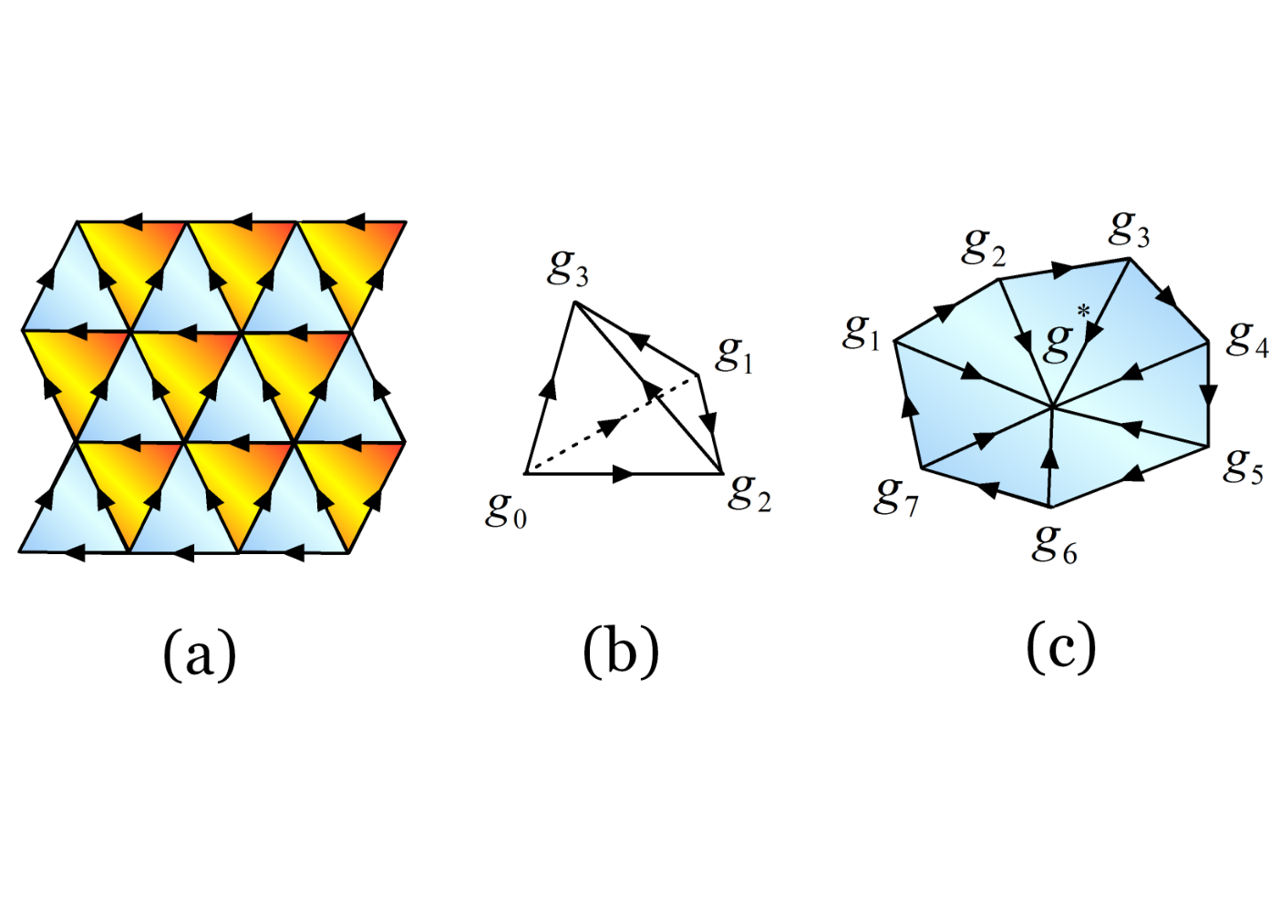
To write the path integral for disordered phases, we first realize that the field of the system fluctuates strongly at all length scales and the low energy effective theory has no continuous limit. Therefore, we choose to write the path integral on discrete space-time. Imagine that we discretize the space time of the Haldane chain with a branched triangularization as shown in Fig.2(a). On each vertex of the space-time complex, we put a . Time reversal acts as complex conjugation together with a mapping from to . The path integral is then written as
| (6) |
is the number of elements in ( for the time reversal symmetry), is the number of vertices in the complex. Also, depending on the orientation of the triangle. Compared to the continuous formulation of path integral corresponds to the field and corresponds to the path integral . is the action-amplitude on the discretized space-time that corresponds to of the continuous formulation and corresponds to the action-amplitude on a single triangle .The above term can be formally regarded as the discrete symmetry group and discrete space time generalization of topological -term for an non-linear sigma model.(For details see appendix C.)
From the properties of , it can be checked that the path integral as defined is symmetric under time reversal symmetry with an action amplitude that is in a fixed point form and is always equal to on a closed surface. First because (see Eq.(2)), the path integral is invariant under time reversal. Secondly, Eq.(3) gives rise to a renormalization flow under which the form of the action amplitude remains invariant (for details see appendix D). Finally, Eq.(3) also guarantees that the action amplitude on a closed space time surface is always . This can be easily verified on the simplest discrete closed surface – a tetrahedron, as shown in Fig.2(b). More complicated closed surfaces are obtained by putting tetrahedrons together, hence the action amplitude will always be . Therefore, we have constructed a quantized topological term for the path integral description of systems with time reversal symmetry on discrete space time.
But how do we know that this quantized topological term describes the SPT order in Haldane chain? This can be made explicit by finding the ground state wave-function of the system from the quantized topological term. The ground state wave-function can be obtained by imaginary time evolution from time until time . In our formulation, this is equivalent to imaginary time path integral on a space-time geometry with a boundary (at time ). Denote the boundary as and the whole manifold (a disk) as . As we are considering a fixed point path integral, it does not matter how big the interior of is and we can reduce it, for example, to just one point as shown in Fig.2 (c).
To obtain the ground state wave-function, we fix the degrees of freedom on and choose an arbitrary configuration, for example , for degrees of freedom in the interior of . We find
| (7) |
where is product over all triangles on and for simplicity of notation we have chosen all triangles to be oriented clockwise. The wave-function on does not depend on the choice of . Note that time reversal acts as complex conjugate together with a change of basis , on each and the wave-function is invariant under this action.

This form of wave-function does not look exactly the same as the dimer form shown in Fig.1, but it will be after a duality transformation as shown in Fig.3. First expand each into two degrees of freedom and such that and the amplitude of each configuration in the wave-function remains unchanged, . Then combine and into one site and apply a change of basis on each site
The amplitude of all configurations in the new basis becomes , which can be equivalently written as a product of dimers between neighboring sites . In this way we have mapped each degree of freedom into a dimer and the total wave-function takes the same form as Eq.(4).
It is also important to check that time reversal symmetry acts as in Eq.(1) on the edge degree of freedom in the ground state. To see this, note that after the duality transformation, time reversal symmetry acts separately on each site and is composed of complex conjugation together with unitary transformation on the basis states
which factorizes on the two degrees of freedom and acts in the same way as in Eq.(1) on the edge. Therefore, our quantized topological term Eq.(6) provides a proper description of the SPT order in the Haldane chain.
The advantage of reformulating the Haldane chain in the path integral language is that it can be easily generalized to all spatial dimensions and all symmetry groups . The two cocycles used in the construction have higher dimensional analogues – the -cocycles , which are maps from group elements to a phase factor and satisfy
A quantized topological term in the path integral of a system can be written in terms of the -cocycles by (1) discretizing the space time with triangularization (triangle in and tetrahedron in etc ); (2) putting group element labeled degrees of freedom onto the vertices (3) assigning action amplitude to each simplex with the corresponding cocycle. The path integral then takes the form
| (8) |
where depending on the orientation of the simplex . Similar to the case, it can be shown that the path integral is symmetric under symmetries in group , the action amplitude is in a fixed point form and is quantized to on a closed manifold.
The ground state wave-function can be obtained from the action amplitude on a open geometry as discussed before , where is on and is inside . is the product over all simplices. An exactly soluble Hamiltonian can be constructed to realize this state as the gapped ground state. To see this, note that can be mapped through a local unitary transformation to a total product state . As is the gapped ground state of , , is the gapped ground state of , which is local and has symmetry .
The nontrivial SPT order of the system can be seen explicitly from its boundary. The path integral of degrees of freedom on the boundary can be obtained by putting the topological term on an open geometry as shown in Fig.2 (c) for . Note that the manifold now corresponds to the space time manifold of the boundary degrees of freedom. The path integral for the boundary then reads
| (9) |
where is the field on and is inside . The action amplitude for each configuration does not depend on the choice of .
This term can be thought of as a discretized version of the Wess-Zumino-Witten(WZW) term[37, 38] in nonlinear -models because 1. it is a path integral of dimensional systems written on an extended manifold with a boundary 2. the action amplitude does not depend on how the extended field in the interior of the manifold is chosen 3. its field takes value in a group and the path integral is invariant under the action of . On the other hand, this term is more general than the original continuous WZW term because it applies to discrete groups like while the continuous WZW term only works for continuous groups. We expect that the boundary theory described by such a discretized WZW term will be gapless as long as symmetry is not broken, similar to systems described by continuous WZW terms. Actually this has been firmly established in and . In , as we have discussed with the example of time reversal symmetry, symmetry action on the edge degree of freedom does not have a one-dimensional representation, therefore the edge state will always be degenerate. In , we have proved rigorously using the tool of matrix product unitary operator that the symmetry action on the boundary requires it to be gapless as long as symmetry is not broken.[39, 40] Therefore, the boundary of the systems we constructed carries gapless excitations protected by certain symmetry, which reflects the nontrivial SPT order of the system.
In conclusion, we have presented a systematic construction of symmetry protected topological phases in bosonic systems in any spatial dimension and with any symmetry of group . In particular, we wrote down a quantized topological term in the path integral of the system based on nontrivial -cocycles of the symmetry group. From the quantized topological term we found that the ground state wave-function is short range entangled and the boundary of the systems carries gapless excitations protected by the symmetry of the system, which clearly demonstrates the nontrivial SPT order of the system. The number of nontrivial cocycles, hence the number of nontrivial SPT phases, for some simple symmetry groups are summarized in table 1. Our construction is non-perturbative and works for strongly interacting bosonic systems.
This research is supported by NSF Grant No. DMR-1005541 and NSFC 11074140. Z.C.G. is supported by NSF Grant No. PHY05-51164.
Appendix A Projective Representation
Matrices form a projective representation of symmetry group if
| (10) |
Here and , which is called the factor system of the projective representation. The factor system satisfies
| (11) |
for all , where if is unitary and if is anti-unitary. If , this reduces to the usual linear representation of .
A different choice of pre-factor for the representation matrices will lead to a different factor system :
| (12) |
We regard and that differ only by a pre-factor as equivalent projective representations and the corresponding factor systems and as belonging to the same class .
Suppose that we have one projective representation with factor system of class and another with factor system of class , obviously is a projective presentation with factor system . The corresponding class can be written as a sum . Under such an addition rule, the equivalence classes of factor systems form an Abelian group, which is called the second cohomology group of and is denoted as . The identity element is the class that corresponds to the linear representation of the group.
can be equivalently expressed as with correspondence
| (13) |
where is the identity element in the symmetry group . satisfies
| (14) |
and the condition Eq.(11) satisfied by becomes
| (15) |
Similarly, can be equivalently written as where
| (16) |
The equivalence relation Eq.(12) between ’s then becomes
| (17) |
In the following we will show defined in Eq.(1) forms a projective representation of symmetry group . It is easy to check that:
with . We note that in the last line, the sign factor arises because the complex conjugate could have a nontrivial action on if is an antiunitary. According to the -cocycle condition Eq. (15), we have:
| (19) |
Now it is clear that defined in Eq.(1) forms a projective representation of the symmetry group . However, is usually reducible. It can be reduced to a direct sum of several irreducible projective representations which belong to the same class. Only irreducible projective representations describe the edge states of general 1D SPT phases.
Appendix B Group cohomology
The above discussion on the factor system of a projective representation can be generalized which gives rise to a cohomology theory of groups. In this section, we will briefly describe the group cohomology theory.
For a group , let be a G-module, which is an abelian group (with multiplication operation) on which acts compatibly with the multiplication operation (ie the abelian group structure) on M:
| (20) |
For the cases studied in this paper, is simply the group and a phase. The multiplication operation is the usual multiplication of the phases. The group action is trivial (, ) if is unitary and if is anti-unitary.
Let be a function of group elements whose value is in the G-module . In other words, . satisfies
| (21) |
We will call such a map an -cochain: Let be the space of all -cochains. Note that is an Abelian group under the function multiplication . We define a map from to :
| (22) |
Let
and
and are also Abelian groups which satisfy where . The -cocycle of is defined as
| (23) |
Let us discuss some simple cases. From
we see that
Since is trivial, . If we define , it is easy to see that the first-cocycle is related to the one-dimensional representations of the group .
From
| (24) |
we see that
and
which give us the 3-cocycle .
Appendix C Relationship with the topological- term of the non-linear sigma model
In the section, we will show the amplitudes Eq.(6) can be formally regarded as the discrete group and discrete space time generalization of topological term of non-linear sigma model. We will first review that the Haldane phase (a non-trivial 1D SPT phase) is described by a -quantized topological term in continuous non-linear -model.[41] However, such kind of -quantized topological terms cannot describe more general 1D SPT phases. We argue that to describe SPT phases correctly, we must generalize the -quantized topological terms to discrete space-time.
Before considering a spin- chain, let us first consider a D non-linear -model that describes a single spin, whose imaginary-time action is given by
| (25) |
where is an unit 3d vector and we have assumed that the time direction form a circle. The second term is the Wess-Zumino-Witten (WZW) term.[37, 38] We note that the WZW term cannot be calculated from the field on the time-circle. We have to extend to a disk bounded by the time-circle: (see Fig. 4). Then the WZW term can be calculated from . When is an integer, WZW terms from different extensions only differ by a multiple of . So is determined by and is independent of how we extend to the disk .

The ground states of the above non-linear -model have fold degeneracy, which form the spin- representation of . The energy gap above the ground state approaches to infinite as . Thus a pure WZW term describes a pure spin- spin.

To obtain the action for the symmetric antiferromagnetic spin-1 chain, we can assume that the spins are described by a smooth unit vector field : (see Fig. 5b). Putting the above single-spin action for different spins together, we obtain the following (1+1)D non-linear -model[42]
| (26) |
where and is the topological term.[42] If the space-time manifold has no boundary, then when . We will call such a topological term – a -quantized topological term. The above non-linear -model describes a gapped phase with short range correlation and the symmetry, which is the Haldane phase.[13] In the low energy limit, flows to infinity and the fixed-point action contains only the -quantized topological term. Such a non-linear -model will be called topological non-linear -model.
It appears that the -quantized topological term has no contribution to the path integral and can be dropped. In fact, the -quantized topological term has physical effects and cannot be dropped. On an open chain, the -quantized topological term becomes a WZW term for the boundary spin (see Fig. 5).[41] The motion of is described by Eq.(25) with . So the Haldane phase of spin-1 chain has a spin-1/2 boundary spin at each chain end![15, 16, 41]
We see that the Haldane phase is described by a fixed point action which is a topological non-linear -model containing only the -quantized topological term. The non-trivialness of the Haldane phase is encoded in the non trivially quantized topological term.[41, 43] From this example, one might guess that various SPT phases can be classified by various topological non-linear -models, and thus by various -quantized topological terms. But such a guess is not correct.
This is because the fixed-point action (the topological non-linear -model) describes a short-range-correlated state. Since the renormalized cut-off length scale of the fixed-point action is always larger than the correlation length, the field fluctuates strongly even at the cut-off length scale. Thus, the fixed-point action has no continuum limit, and must be defined on discrete space-time. On the other hand, in our fixed-point action, is assumed to be a continuous field in space-time. The very existence of the continuum -quantized topological term depends on the non-trivial mapping classes from the continuous space-time manifold to the continuous target space . It is not self consistent to use such a continuum topological term to describe the fixed-point action for the Haldane phase.
As a result, the continuum -quantized topological terms fail to classify bosonic SPT phases. For example, different possible continuum -quantized topological terms in Eq.(26) are labeled by integers, while the integer spin chain has only two gapped phases protected by spin rotation symmetry: all even-integer topological terms give rise to the trivial phase and all odd-integer topological terms give rise to the Haldane phase. Also non-trivial SPT phases may exist even when there is no continuum -quantized topological terms (such as when the symmetry is discrete).
However, the general idea of using fixed-point actions to classify SPT phases is still correct. But, to use -quantized topological terms to describe bosonic SPT phases, we need to generalize them to discrete space-time. In the following, we will show that this indeed can be done, using the (1+1)D model (26) as an example.
A discrete (1+1)D space-time is given by a branched triangularization (see Fig. 2 (a)). Since , on triangularized space-time, we can rewrite
| (27) |
where is the action on a single triangle. We see that, on discrete space-time, the action and the path integral are described by a 3-variable function , which is called action amplitude. The symmetry requires that
| (28) |
In order to use the action amplitude to describe a -quantized topological term, we must have on any sphere. This can be satisfied iff on a tetrahedron – the simplest discrete sphere (See Fig. 2(b)):
| (29) |
(Another way to define topological term on discretized space-time can be found in .)
A that satisfies Eq.(28) and Eq.(29) is called a 2-cocycle. If is a 2-cocycle, then
| (30) |
is also a 2-cocycle, for any satisfying , . Since and can continuously deform into each other, they correspond to the same kind of -quantized topological term. So we say that and are equivalent. The equivalent classes of the 2-cocycles give us – the 2-cohomology group of sphere with coefficient. classifies the -quantized topological term in discrete space-time and with as the target space.
Does classify the SPT phases with symmetry? The answer is no. We know that is just one of the symmetric spaces of . To classify the SPT phases, we need to replace the target space by the maximal symmetric space, which is the group itself (see for more discussions). So we need to consider discrete non-linear -model described by , . Now the 2-cocycle conditions becomes
| (31) |
which defines a “group cohomology” . It classifies the -quantized topological term for the maximal symmetric space. It also classifies the SPT phases with symmetry in (1+1)D.
Appendix D Branched triangulation and topological invariant amplitudes
As we have shown, the bosonic symmetry protected order in D can be described by the amplitude:
| (32) |
where are group elements of the symmetry group and is the order of . The -cocycle is defined on the branched -simplex, with uniquely determined by the orientation of the corresponding -simplex. In the following, we will show they are topological invariant amplitudes. Hence, they represent a class of fixed point amplitudes of (symmetry protected) topologically ordered phases.
First, we need to give a branching structure to the discretized space-time. A branching is a choice of an orientation of each edge of an -simplex such that there is no oriented loop on any triangle. For example, Fig. 6 (a) is a branched -simplex and (c) is a branched -simplex. However, (b) is not an allowed branching because all its three edges contain the same orientations and thus form an oriented loop. (d) is also not allowed because one of its triangle contains an oriented loop. It is easy to check that any consistent branched structure can induce a canonical ordering for the vertices of -simplex. Indeed, the branching structure will also induce an canonical orientation of the -simplex, see Fig. 7.
To understand the geometric meaning of the topological invariance of the above amplitude, let us first discuss (1+1)D fixed-point action-amplitude with a symmetry group . For a D system on a complex with a branching structure, a fixed-point action-amplitude (see Fig. 8)
| (33) |
where each triangle contribute to a phase factor , multiply over all the triangles in the complex Fig. 8. Note that the first variable in correspond to the vertex with two out going edges, the second variable to the vertex with one out going edges, and the third variable to the vertex with no out going edges. depending on the orientation of to be anti-clock-wise or clock-wise.
In order for the action-amplitude to represent a quantized topological -term, we must choose such that
| (34) |
on closed space-time complex without boundary, in particular, on a tetrahedron with four triangles (see Fig. 2(b)):
| (35) |
Also, in order for our system to have the symmetry generated by the group , its action-amplitude must satisfy
| (36) |
where is the time-reversal transformation. This requires
| (37) |
Eq.(36) and Eq.(37) happen to be the conditions of 2-cocycles of . Thus the action-amplitude Eq.(33) constructed from a 2-cocycle is a quantized topological -term.
If satisfy Eq.(36) and Eq.(37), then
| (38) |
also satisfy Eq.(36) and Eq.(37), for any satisfying , . So also gives rise to a quantized topological -term. As we continuously deform , the two quantized topological -terms can be smoothly connected. So we say that the two quantized topological -terms obtained from and are equivalent. We note that and differ by a 2-coboundary . So the equivalence classes of is nothing but the cohomology group . Therefore, the quantized topological -terms are classified by .
We can also show that Eq.(33) is a fixed-point action-amplitude from the cocycle conditions on . The cocycle condition Eq.(35) induces two renormalization moves in the discretized manifold. Fig. 9 represents a moves:
| (39) |
and Fig. 10 represents a move:
| (40) |
By using these two moves, different triangularization of the space-time can be mapped into each other without changing the action amlitude Eq.(32). Therefore, the action-amplitude is a fixed point form.
Geometrically, these two moves can be obtained by projecting a 3 simplex onto two two-dimensional surfaces. Fig.11 (a) gives the move and Fig.11 (b) gives the move. Note that the projection from opposite directions will induce opposite chiralities for the boundary of the tetrahedron, that’s why we need to change the chiralities of the triangular in one side of basic moves. Such a change correspond to inverse when we move it from left side to right side of the above equation, which is consistent with our rules of algebra. Similar process also works in higher dimensions. Different moves in -dimension can be obtained from projecting a -simplex in different ways. Such moves induces a renormalization flow in the discrete space-time under which the action-amplitude Eq.(32) is a fixed point.
References
- [1] L. D. Landau, Phys. Z. Sowjetunion 11, 26 (1937).
- [2] V. L. Ginzburg and L. D. Landau, Zh. Ekaper. Teoret. Fiz. 20, 1064 (1950).
- [3] L. D. Landau and E. M. Lifschitz, Statistical Physics - Course of Theoretical Physics Vol 5 (Pergamon, London, 1958).
- [4] A. Kitaev and J. Preskill, Phys. Rev. Lett. 96, 110404 (2006).
- [5] M. Levin and X.-G. Wen, Phys. Rev. Lett. 96, 110405 (2006).
- [6] X. Chen, Z.-C. Gu, and X.-G. Wen, Phys. Rev. B 82, 155138 (2010).
- [7] X. G. Wen, International Journal of Modern Physics B 4, 239 (1990).
- [8] X. G. Wen and Q. Niu, Phys. Rev. B 41, 9377 (1990).
- [9] Z.-C. Gu and X.-G. Wen, Phys. Rev. B 80, 155131 (2009).
- [10] D. C. Tsui, H. L. Stormer, and A. C. Gossard, Phys. Rev. Lett. 48, 1559 (1982).
- [11] R. B. Laughlin, Phys. Rev. Lett. 50, 1395 (1983).
- [12] X.-G. Wen, Advances in Physics 44, 405 (1995), eprint http://www.tandfonline.com/doi/pdf/10.1080/00018739500101566.
- [13] F. D. M. Haldane, Physics Letters A 93, 464 (1983a).
- [14] I. Affleck, T. Kennedy, E. H. Lieb, and H. Tasaki, Communications in Mathematical Physics 115, 477 (1988), ISSN 0010-3616, 10.1007/BF01218021.
- [15] M. Hagiwara, K. Katsumata, I. Affleck, B. I. Halperin, and J. P. Renard, Phys. Rev. Lett. 65, 3181 (1990).
- [16] S. H. Glarum, S. Geschwind, K. M. Lee, M. L. Kaplan, and J. Michel, Phys. Rev. Lett. 67, 1614 (1991).
- [17] T.-K. Ng, Phys. Rev. B 50, 555 (1994a).
- [18] F. Pollmann, E. Berg, A. M. Turner, and M. Oshikawa, Phys. Rev. B 85, 075125 (2012).
- [19] X. Chen, Z.-C. Gu, and X.-G. Wen, Phys. Rev. B 83, 035107 (2011a).
- [20] L. Fidkowski and A. Kitaev, Phys. Rev. B 83, 075103 (2011).
- [21] A. M. Turner, F. Pollmann, and E. Berg, Phys. Rev. B 83, 075102 (2011).
- [22] N. Schuch, D. Perez-Garcia, and I. Cirac, Phys. Rev. B 84, 165139 (2011).
- [23] C. L. Kane and E. J. Mele, Phys. Rev. Lett. 95, 226801 (2005a), eprint cond-mat/0411737.
- [24] B. A. Bernevig and S.-C. Zhang, Phys. Rev. Lett. 96, 106802 (2006).
- [25] C. L. Kane and E. J. Mele, Phys. Rev. Lett. 95, 146802 (2005b), eprint cond-mat/0506581.
- [26] J. E. Moore and L. Balents, Phys. Rev. B 75, 121306 (2007), eprint cond-mat/0607314.
- [27] L. Fu, C. L. Kane, and E. J. Mele, Phys. Rev. Lett. 98, 106803 (2007), eprint cond-mat/0607699.
- [28] X.-L. Qi, T. L. Hughes, and S.-C. Zhang, Phys. Rev. B 78, 195424 (2008).
- [29] A. Kitaev, AIP Conference Proceedings 1134, 22 (2009).
- [30] S. Ryu, A. P. Schnyder, A. Furusaki, and A. W. W. Ludwig, New Journal of Physics 12, 065010 (2010).
- [31] L. Fidkowski and A. Kitaev, Phys. Rev. B 81, 134509 (2010).
- [32] Z. C. Gu and X.-G. Wen (2012), eprint 1201.2648.
- [33] X.-L. Qi (2012), eprint 1202.3983.
- [34] Z. C. Gu and M. Levin (2012), eprint to appear.
- [35] H. Yao and S. Ryu (2012), eprint 1202.5805.
- [36] S. Ryu and S.-C. Zhang (2012), eprint 1202.4484.
- [37] J. Wess and B. Zumino, Physics Letters B 37, 95 (1971), ISSN 0370-2693.
- [38] E. Witten, Nuclear Physics B 223, 422 (1983), ISSN 0550-3213.
- [39] X. Chen, Z.-X. Liu, and X.-G. Wen, Phys. Rev. B 84, 235141 (2011b).
- [40] M. Levin and Z. C. Gu (2012), eprint 1202.3120.
- [41] T.-K. Ng, Phys. Rev. B 50, 555 (1994b).
- [42] F. D. M. Haldane, Phys. Rev. Lett. 50, 1153 (1983b).
- [43] A. P. Schnyder, S. Ryu, A. Furusaki, and A. W. W. Ludwig, Phys. Rev. B 78, 195125 (2008).
- [44] N. Seiberg, Phys. Rev. Lett. 53, 637 (1984).
- [45] X. Chen, Z.-C. Gu, Z.-X. Liu, and X.-G. Wen, ArXiv e-prints (2011), eprint 1106.4772.