Bootstrap Testing of the Rank of a Matrix via Least Squared Constrained Estimation.
Abstract
In order to test if an unknown matrix has a given rank (null hypothesis), we consider the family of statistics that are minimum squared distances between an estimator and the manifold of fixed-rank matrix. Under the null hypothesis, every statistic of this family converges to a weighted chi-squared distribution. In this paper, we introduce the constrained bootstrap to build bootstrap estimate of the law under the null hypothesis of such statistics. As a result, the constrained bootstrap is employed to estimate the quantile for testing the rank. We provide the consistency of the procedure and the simulations shed light one the accuracy of the constrained bootstrap with respect to the traditional asymptotic comparison. More generally, the results are extended to test if an unknown parameter belongs to a sub-manifold locally smooth. Finally, the constrained bootstrap is easy to compute, it handles a large family of tests and it works under mild assumptions.
Keywords. Rank estimation, Least squared constrained estimation, Bootstrap, Hypothesis testing.
1 Introduction
Let be an unknown matrix (arbitrarily ). To infer about the rank of with hypothesis testing, the general framework usually considered is the following: there exists an estimator of such that
| (1) |
where vectorizes a matrix by stacking its columns. In the whole paper the hatted quantities are random sequences that depends on the sample number , all the limit are taken with respect to . Moreover there exists an estimator such that
| (2) |
and in some cases, one may ask that
| (3) |
Let be the rank of and , we consider the set of hypotheses
| (4) |
Thus can be estimated the following way: we start by testing , if is rejected we go a step further , if not we stop the procedure and the estimated rank is . In this paper, by considering the hypotheses (4) we focus on each step of this procedure.
Many different statistical tests appeared in the literature for this purpose. For instance Cragg and Donald [11] introduced a statistic based on the LU decomposition of , Kleibergen and Paap [19] studied the asymptotic behaviour of some transformation of the singular values of , and Cragg and Donald [12] considered the minimum of a squared distance under rank constraint. In some other fields with similar issues, close ideas have been developed : Bura and Yang [7] examined a Wald type statistic depending on the singular decomposition of and Cook and Ni [10] also considered the minimum of a squared distance under rank constraint. Although based on different considerations, each of the previous work relies on the test described by (4). For comprehensiveness, in this paper we consider the following three statistics. The first one is introduced by Li [21] as
| (5) |
where are the singular values of arranged in descending order. Under and (1), this statistic converges in law to a weighted chi-squared distribution [7]. The main drawback of such a test is that is not pivotal, i.e. its asymptotic law depends on unknown quantities that are and . Accordingly the consistency of the associated test requires assumptions (1) and (2). In [7] a standardized version of is studied with
| (6) |
where stands for the Moore-Penrose inverse of and and are respectively the orthogonal projectors on the left and right singular spaces associated with the smallest singular values of . The authors proved that under , if (1) and (2) hold, the Wald-type statistic is asymptotically chi-squared distributed. Besides, [12] and [10] proposed a constrained estimator by minimizing a squared distance under a fixed-rank constraint as
| (7) |
which is also asymptotically chi-squared distributed under , assuming (1), (2) and (3). We will refer the minimum discrepancy approach. Although the statistics and have the convenience of being pivotal, they both require the inversion of a large matrix and this may cause robustness problems when the sample number is not large enough. For and under the relevant assumptions, each of these statistics , and , is consistent at level in testing (4), i.e. the level goes to and the power goes to as goes to .
Nevertheless the estimation of the quantile is difficult because either the asymptotic distribution depends on the data (non pivotality represented by ), or the true distribution may be quite different than the asymptotic one (slow rates of convergence represented by and ). The objective of the paper is to propose a bootstrap method for quantile estimation in this context.
An important remark which instigates the sketch of the paper is that all the previous statistics share the form
| (8) |
where is the Euclidean norm, , . The values of and corresponding to the statistics , and are summarized in the Table 1 (See Section 2 for the details).
We refer to traditional testing (resp. bootstrap testing) when the statistic is compared to its asymptotic quantile (resp. bootstrap quantile). The bootstrap test is said to be consistent at level if
| (9) |
where is the quantile of level calculated by bootstrap. The advantage of bootstrap testing is its high level of accuracy under with respect to traditional testing. This fact is emphasized by considering the two possibilities: when the statistic is pivotal and when the asymptotic law of the statistic depends on unknown quantities. First, as highlighted by Hall [15], when the statistic is pivotal, under some conditions the gap between the distribution of the statistic and its bootstrap distribution is . Since the normal approximation leads to a difference , the bootstrap enjoys a better level of accuracy. Secondly if the asymptotic law of the statistic is unknown, the bootstrap appears even more as a convenient alternative because it avoids its estimation. In [17], Hall and Wilson give two advices for the use of the bootstrap testing:
- A)
Whatever the sample is under or , the bootstrap estimates the law of the statistic under .
- B)
The statistic is pivotal.
The first guideline is the most crucial because if it fails it may lead to inconsistency of the test. The second guideline aims at improving the accuracy of the test by taking full advantage of the accuracy of the bootstrap. In this paper we propose a new procedure for bootstrap testing in least square constraint estimation (LSCE) (estimators as (8) are particular cases), called constrained bootstrap (CS bootstrap). More precisely, the CS bootstrap aims at testing whether a parameter belongs or not to a submanifold and so generalised the test (4). Our main result is the consistency of the CS bootstrap under mild conditions. As a consequence we provide a consistent bootstrap testing procedure for testing (4) with the statistic , and . For the sake of clarity, we address the CS bootstrap in the next section. Section 3 is dedicated to rank estimation with special interest to the bootstrap of the statistic , and . Finally, the last section emphasizes the accuracy of the bootstrap in rank estimation by providing a simulation study in sufficient dimension reduction (SDR). Accordingly, the sketch of the paper is as follows:
The CS bootstrap in LSCE
Bootstrap testing procedure for , and
Application to SDR
2 The constrained bootstrap for LSCE and hypothesis testing
Because of (8) LSCE has a central place in the paper. Moreover since LSCE intervenes in many statistical fields as M-estimation or hypothesis testing, this section is independent from the rest of the paper.
2.1 LSCE
Let be called the parameter of interest, and let be an estimator of . We define the constrained estimator of as
| (10) |
where is a submanifold of with co-dimension , and . The constrained statistic is defined as
| (11) |
where . Note that if is full rank, the unique minimizer of (10) without constraint is , hence it could be understood as the unconstrained estimator. We introduce now the notion of nonsingular point in . This one is needed to express the Lagrangian first order condition of the optimization (10). For any function , define its Jacobian as , where stands for the gradient operator.
Definition 1.
We say that is -nonsingular if and if there exists a neighbourhood and a function continuously differentiable on with full rank such that
As a consequence any point of a submanifold locally smooth is nonsingular, e.g. any matrix with rank is a nonsingular point in the submanifold . We prove in Proposition 2 that if is -nonsingular, and is full rank, then we have
| (12) |
where the ’s are i.i.d. Gaussian random variables and the ’s are the eigenvalues of the matrix . Especially, the case is interesting because is asymptotically chi-squared distributed with degrees of freedom. Otherwise, if , goes to infinity in probability. Those facts shed light on a consistent testing procedure based on LSCE with the hypotheses
| (13) |
and the decision rule to reject if is larger than a quantile of its asymptotic law. Accordingly the previous framework can be seen as an extension of the Wald test statistic which handles the simple hypothesis with the statistic .
2.2 The bootstrap in LSCE
Since LSCE is a particular case of estimating equation, we review the bootstrap literature with two principal directions: estimating equation and hypothesis testing. For clarity we alleviate the framework in this section: let be an i.i.d. sequence of real random variables with law , define , , we put , , and where stands for the empirical mean.
The original bootstrap was introduced in [14] in the following way. Let be an i.i.d. sequence of real random variables with law , define , the distribution of conditionally on the sample, that we call the bootstrap distribution, is “close” to the distribution of , that we call the true distribution (in the rest of the paper we just say “conditionally” instead of “conditionally on the sample”). For instance, it is shown in [23] that the bootstrap distribution converges weakly to the true distribution almost surely. One says that bootstraps and we will write
where and both mean the asymptotic laws with the difference that the later is conditional on the sample. Equivalently, one has for every , , but the use of the bootstrap is legitimate by a more general results stated in [15], which says that
| (14) |
with , provided that is non-lattice. Besides, one has
where is the cumulative distribution function (c.d.f.) of the standard normal law. Variations of Efron’s resampling plan are proposed in [2] under the name of weighted bootstrap. For a complete introduction about the bootstrap we refer to [15]. We now present three different bootstrap techniques related to LSCE11 1 A bootstrap with a Delta-method approach (see [23], chapter 23, Theorem 5) fails because is not continuously differentiable on the unit circle..
- (i)
The classical bootstrap (C bootstrap)
The literature about the bootstrap in Z and M-estimation, see respectively [9] and [1], is based on the following principle: if is estimated by where is an open set, then the bootstrap of is carried out by the quantity with
(15) where is a sequence of random variables. The particular case where the vector is distributed as leads to a direct application of original Efron’s bootstrap to M-estimation. Since such a bootstrap has been extensively studied, we refer to the C bootstrap. To the knowledge of the authors, the C bootstrap when has empty interior has not been studied yet. Nevertheless one may sight its bad behaviour for the test of equal mean . The associated least squared constrained statistic
is indeed the score statistic associated to the M-estimator with and . Clearly the C bootstrap through does not work because of its bad behaviour under for instance. In this case it is better to use
but it cannot handle the cases of more involved hypotheses22 2 We refer to [17] for a study of this bootstrap in order to test .. Whereas the C bootstrap is not really connected with hypothesis testing, the two following bootstrap procedures are more related to the present work.
- (ii)
The biaised bootstrap (B bootstrap)
The B bootstrap is introduced in [16] and is directly motivated by hypothesis testing. The original idea of their work is to re-sample with respect to the distribution , where the ’s maximize
Since the ’s minimize the Kulback-Leibler distance between and , one can see the resulting distribution as the closest to the original one satisfying the mean constraint. The authors presented interesting results for the test of equal mean , essentially the bootstrap statistic , with , sampled from , has a chi-squared limiting distribution either or is assumed. As a result both guidelines (A) and (B) are checked. They go further by showing that the B bootstrap outclasses the asymptotic normal approximation for quantile estimation in the sense that whereas , where , and are the quantile functions of the standard normal distribution, the statistic under and the bootstrapped statistic, respectively. Although the B bootstrap matches the context of hypothesis testing, it has been designed to handle the particular test of equal mean. To the knowledge of the authors the study of the B bootstrap has not been extended to other tests. Facing (ii), the main drawback of the B bootstrap deals with algorithmic difficulties. Indeed when the constraint becomes more involved, solving (ii) is more difficult. As a result it is not sure that this method could handle other situations such as fixed-rank constraints.
- (iii)
The estimating function bootstrap (EF bootstrap)
Now . Some other ideas about the bootstrap of the -estimators can be found in [20] and [18], and can be summarized as follows. Considering the score statistic , [18] showed that it could be bootstrapped by
where is a sequence of random variables. This bootstrap is called the EF bootstrap and revealed nice computational properties. Moreover the authors argued for its use in quantile estimation in order to test if , where is the constraint function, by recommending essentially to use . Applying it to the least squared context , the EF bootstrap is carried out by
Although it verifies both guidelines (A) and (B) (see the article for details), one can see that the good behaviour of such an approach is more based on the rank deficiency of than on the bootstrap of . Indeed bootstraps the non constrained estimator . Then as the authors noticed, it is first of all a bootstrap of the Wald-type statistic which has fortunately the same asymptotic law than the targeted one. This may induce some loss in accuracy. Moreover, it requires the knowledge of the function which is not the case for fixed rank constraints where the depends on the limit (see Remark 1 for some details).
Essentially both (i) and (ii) provide a bootstrap for testing simple hypotheses. The EF bootstrap proposed in (iii) extends this limited scope by including tests of the form where is known. Nevertheless it does not handle the test (4) as it is highlighted by the following remark.
Remark 1.
Testing (4) with results in an optimization with the constraint . Since the subspace of fixed rank matrices is a submanifold locally smooth with co-dimension , at every point , there exists a neighbourhood and a function such that and has full rank. Moreover, we have
If now (1) holds, the right-hand side term goes to in probability and . As a consequence, if is invertible, for any neighbourhood of , from a certain rank, belongs to it with probability . Then under since has rank the constrained estimator has the expression
with depending on . Unfortunately we do not know neither nor . This entails some problems relating to the later approach.
2.3 The constrained bootstrap
The CS bootstrap is introduced in order to solve all the issues we have raised through the previous little review which are essentially: computational difficulties and small scope of the existing methods. The CS bootstrap targets an estimation of the quantile under of . The consistency of the procedure, i.e. (9), forms the main result about the CS bootstrap. Another important issue which occurs beforehand in the section is the bootstrap of the law of
Basically, we show that a bootstrap of the unconstrained estimator allows a bootstrap of the constrained estimator under . We point out that the CS bootstrap heuristic is rather different than the C and EF bootstrap. Otherwise it shares the idea to “reproduce” even if is realized with the B bootstrap. Assuming that we can bootstrap , the CS bootstrap calculation of the statistic is realized as follows:
The CS bootstrap procedure Compute (18) where the simulation of can be done by a standard bootstrap procedure33 3 The bootstrap procedure to get is not specified because it depends on . For instance, if is a mean over some i.i.d. random variables, one can use the Efron’s traditional bootstrap and if is a M-estimator, one should use a bootstrap as detailed by equation (15).. Calculate (19) where and 44 4 Assumptions about and are provided further in the statements of the propositions..
Intuitively, this choice appears natural because equals plus a small perturbation going to . Accordingly is somewhat reproducing the behaviour of under , especially because has the right asymptotic variance. As we should notice, and could be chosen as and but this is not the best choice in practice. As it is highlighted in (14), we should normalized by the associated bootstrap quantities (e.g. the variance computed on the bootstrap sample). The following lemma gives a first order decomposition of the bootstrap law under mild conditions. The following lemma is proved in the Appendix.
Lemma 1.
Let be a submanifold. Assume there exists and a -nonsingular point such that . If moreover exists a.s. and conditionally a.s. is full rank, then we have conditionally a.s.
with .
Note that if is -nonsingular and exists, we can apply Lemma 1 with . This gives the following proposition:
Proposition 2.
Let be a submanifold. Assume that exists with -nonsingular. Assume also that is full rank, then we have
with .
Proposition 2 leads easily to (12) and extends classical results [6] about constrained estimators with constraint to manifold type constraints. Besides statements of Lemma 1 and Proposition 2 together explain the preceding definition of in (18). They also lead to the following theorem.
Theorem 3.
Let be a submanifold. Assume that with -nonsingular and hold. If moreover (18) holds and conditionally a.s. is full rank, then we have
Essentially, Theorem 3 is an application of Lemma 1 under , indeed as we seen in the proof of Lemma 1, equation (25), the assumption implies that . Nevertheless under nothing guarantee such a convergence (see Example 1 below). Roughly speaking, asking for an equality in law under as in Theorem 3 may be too much to ask. However as stated in the following theorem we do not require that converges a.s. to a constant to provide that the power of the corresponding test goes to . This leads to the consistency of the CS bootstrap for hypothesis testing. For the statement of the consistency theorem, we need to define the quantile function of the bootstrap statistic
where is the c.d.f. of conditionally on the sample.
Theorem 4.
Let be a manifold. Assume that with -nonsingular under . We assume also that is full rank, . If moreover a.s. has a density, and conditionally a.s. , , then we have
In other words, the test described in (13) with statistic and CS bootstrap calculation of quantile is consistent.
We provide the following example under , where does not converge to a constant in probability. Although we cannot get the conclusion of Theorem 3, the least squared constrained statistic still converges in distribution.
Example 1.
Let be a i.i.d. sequence such that . Define , and . Clearly does not hold and naturally the statistic goes to infinity in probability. One can find that which does not converge. Since
we get that a.s. and naturally, we do not have the asymptotic given by Theorem 3. Besides, the convergence to a chi-squared distribution holds for the quantity .
3 Rank estimation with hypothesis testing
In this section through a review of the literature about rank estimation, we apply the results obtained in section 2.1 to provide a consistent bootstrap procedure for the test described by (4) associated with the statistics , and . We define the dimension of the kernel of . We denote by the singular values of arranged in descending order and we write the SVD of as
with , , , , and . For , we note and we write the SVD of as
with , , , , and . We also introduce the orthogonal projectors
Whereas the link between and LSCE is evident, the one conecting and to LSCE relies on the following classical lemma, whose proof is avoided.
Lemma 5.
Let , it holds that
where are the singular values of arranged in descending order, and and are orthogonal right and left singular projectors of associated with .
Note that in the previous lemma, and are uniquely determined if and only if .
3.1 Nonpivotal statistic
As stated in the introduction, the statistic can be used to arbitrate between the hypotheses of (4). Basically, if is realized, all the eigenvalues of the sum goes to and has a weighted chi-squared limiting distribution. Otherwise, at least one eigenvalue converges in probability to a positive number and for any , . The following proposition describes the asymptotic behaviour of 55 5 A similar proposition can be stated applying Proposition 12. Following this way, the asymptotic depends on which is difficult to estimate for rank constraints (see Remark 1).. It was stated in [8] and some recent extension can be found in [7]. Our statement goes further because we are also concerned about the estimation of the asymptotic law of , i.e. the estimation of the weights that intervenes in the weighted chi-squared asymptotic law. Besides, the proof we give in the Appendix is quite simple66 6 We no longer need the results of [13] about the asymptotic behaviour of singular values..
Proposition 6.
Remark 2.
Unlike Theorem 1 in [8] or Theorem 1 in [7], we prefer to state this theorem with the quantities and rather than with and . Because we do not assume that the kernel of has dimension , the vectors that form or are not unique because vector spaces with dimension larger than have an infinite number of basis. As a consequence it does not make sense to estimate either or . To characterize convergence of spaces, a suitable object is their associated orthogonal projectors.
In general, we do not know the asymptotic distribution of because it depends on . On the first hand, one can estimate consistently this matrix to get an approximation of the law of under . Some conditions providing the consistency of the estimation are stated in Proposition 6. On the other hand, one can apply the CS bootstrap to estimate the quantile of in order to test. The main advantage of such an approach is that we no longer need to have a consistent estimator of so that (2) is not needed anymore. Following section 2.1 and by using Lemma 5, we define
| (20) |
with defined in (1). Accordingly, we introduce the CS bootstrap statistic
with the smallest singular values of . The following proposition is a straightforward application of Theorem 4 with the submanifold .
3.2 Wald-type statistic
The Wald-type statistic has been introduced in [7] to get a pivotal statistic77 7 We write the expression of another way for the reasons explained in Remark 2 but one can recover the original expression by noting that for any symmetric matrix , if is an orthonormal basis of a vector subspace of .. They obtained the following theorem for which we provide a different proof in the appendix.
3.3 Minimum Discrepancy approach
Noting that has co-dimension and applying (12) we get the following proposition88 8 See [12] for the original proof..
In general a minimizer
does not have an explicit form as it was for the constrained matrix associated with and . Therefore, we define
| (21) |
where is defined in (1). We also define the associated CS bootstrap statistic
and applying Theorem 4 we have the following result.
Proposition 11.
Remark 3.
The set of assumptions needed to obtain Proposition 10 is stronger than the ones stated in propositions 6 and 8 ensuring the convergence of and . As a consequence this is also true for Proposition 11 with respect to propositions 7 and 9. The main difference is that we add the assumption on to be non deficient. This assumption cannot be alleviated in the statement but is not as restrictive in practice. On the first hand, if is deficient the optimization under constraint has a free coordinate which implies the non-convergence of the minimizer. On the other hand, because of the semi-definite character of the projection of on the null space of is null. Then one can apply the proposition to the restriction of on the range of . This is the case in the application to SDR in Section 4.
Remark 4.
Unlike the situation of and , an optimization algorithm is needed to obtain and , this point out an important issue of such a procedure. In [10], the authors noticed that
where is the set of orthogonal basis lying in with dimension . We follow their algorithm in the computation of (see [10], Section 3.3 for the details).
3.4 The statistics , , through an example
In the introduction, we already mentioned several drawbacks and advantages of the use of , , or . The remark relied on both pivotality of the statistics and large matrix inversion. Here we develop another point of view related to the algebraic nature of the statistics. Facing the representation provided by Table 1, each statistic and evaluates a different distance between and . The first one is the distance that is optimized, but the second is another one. This has raised the issue we present here through the following example. For the sake of clarity, we consider
and we test against . We assume that , we have . Otherwise, one can show that , with . For it is clear that the minimization can be done over the diagonal matrix and one has
Accordingly, by Proposition 7, 9 and 11, the three tests can be summarized by
where . Assume there is less variance on the estimate of the smallest eigenvalue, i.e. such that , this situation may arise when and have similar values but different variances. Then to conduct the test, the statistic is a better choice than . As a consequence, unlike and , the statistic appears as a coherent choice because its associated minimization takes into account the variance of the estimation.
4 Application to sufficient dimension reduction
We focus on a particularly famous method in SDR called sliced inverse regression (SIR) which has been introduced in [21] to deal with the regression model
| (22) |
where , , and is a projector on the vector space with dimension , called the central subspace. The objective is to estimate . If is elliptically distributed, then we have that with , for any measurable function . Accordingly, in order to recover the whole central subspace one needs to consider many functions . For a given family of functions we define . Under some additional conditions [22], the image of the matrix is equal to . Then one can make the svd of an estimator of this matrix to obtain vectors that form an estimated basis of . Motivated by the curse of dimensionality, the estimation of is one of the most crucial points in SDR. To make that possible, a popular way consists in estimating the rank of using the hypothesis testing framework given by (4) (see for example [21], [8] and [10]). Since we are interested in estimating the rank, we prefer to deal directly with to avoid the introduction of an additional noise due to the estimation of the matrix . Assume that is a i.i.d. sequence from model (22), denote by its associated empirical c.d.f. and define the quantity
associated with its empirical estimator
We apply the CS bootstrap to calculate the quantiles of each statistic. Facing (20) and (21), we use an independent weighted bootstrap to reproduce the asymptotic law of , that is we define the bootstrap matrix
| (23) |
where stands for the solution of an optimization problem depending on the selected statistic , or (see Section 3 for the details) and is a sequence of i.i.d. random variables. We also define
To apply propositions 7, 9, and 11, we need the following result which is of particular interest since it provides a new bootstrap procedure for SIR that is different than the one proposed in [3].
Proposition 12.
Assume that , and are finites, if moreover is a i.i.d. sequence of real random variables with mean and variance , then we have
Remark 5.
Taking a partition of the range of we recover the original SIR method with the family formed by the ’s with . Then with and , is estimated by with , , . We have the expansion
As a consequence, the matrix and the weights ’s are playing an important role on the asymptotic of the matrix SIR. They introduce some other terms in the asymptotic distribution and clearly the simple bootstrap presented before does not work for SIR as it was originally defined. Even if we believe that a more evolved weighted bootstrap works to bootstrap , we emphasize that it may be less accurate than the one we propose since it complicates the asymptotic without being necessary for testing the rank.
Recall that is a non-negative integer, for and we calculate independent copies with the CS bootstrap algorithm corresponding to each statistic. Then we estimate the quantile with
is the integer ceiling function and stands for the rank statistic associated to the sample . On the first hand, we conduct the test described by (4) using the CS bootstrap, i.e.
| (24) |
On the other hand, the traditional test is conducted by comparing the statistic and to the quantile of their asymptotic law respectively given by propositions 8 and 10. For , in general the limit in law is quite complicated99 9 When the predictors are normally distributed, it has been shown that is asymptotically chi-squared distributed (see [8]). The authors also pointed out that it was less robust than the weighted chi-squared asymptotic as soon as the predictors distribution deviates from normality. As a result, we keep in the nonparametric framework by avoiding such asymptotic in this simulation study. (see Proposition 6), so that we use approximations: the Wood’s approximation (see [24]) as it is computed in the R software, an adjusted version , with , , and a re-scaled version , (see [4] for these two corrections).
In all the simulations we compute the matrix by taking where the ’s form an equi-partition of the range of the data . In the whole study we put , and we consider . Although the parameter does not really affect the SIR method, we choose it globally good with respect to all the situations.
The first model we study is the following standard model:
In order to highlight guidelines (A) and (B), we produce in figure 1 two graphics each representing situation under and for the statistic . Similar graphics dealing with have been drawn but are not presented here.
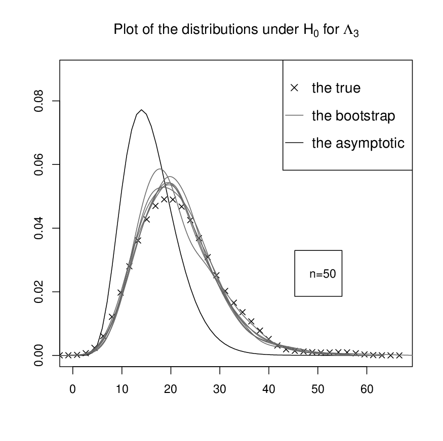

On the first one we see that even if the sample is under the bootstrap distribution reflects . As a consequence, guideline (A) is satisfied and the power of the bootstrap test is going to . The second graph shows that the statistic distribution is closer to the bootstrap distribution than its asymptotic distribution. This has no reason to occur when the statistic is not pivotal (see the introduction and [15] for the details). As a consequence, we believe that this good fitting is due to Guideline B.
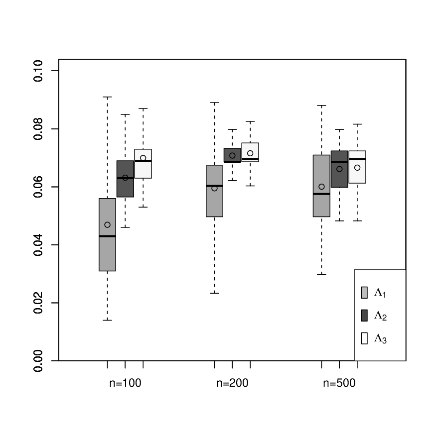
In figure 2 we analyse the asymptotic distribution of in model I for each statistic. To measure the error we consider the behaviour of
which is optimally equal to . To make that possible, is estimated with a large sample size so that the estimation error is negligible. Then we run over samples the CS bootstrap to provide, for each sample, a bootstrap estimation of the quantile . The associated boxplot for , , are provided in Figure 2. As a consequence, we may notice that the behaviour of and are quite similar facing the one of . Even if every boxplot argues for convergence to , testing with seems a better choice when n is small because of a quasi immediate convergence of the bias. When n increase, this is no longer evident because the variance of either or is smaller.
Furthermore, we go into details in Table 2 by running Model I over samples. For each of them and every statistic, we conduct the bootstrap test (24) and its traditional version. The table presents for each , the proportion of rejected tests. This corresponds to either estimate of the power or estimate of the level.
| Wood | Resc. | Adj. | CB | CB | CB | ||||
|---|---|---|---|---|---|---|---|---|---|
| 0.9988 | 0.9998 | 0.9988 | 0.9988 | 1.0000 | 1.0000 | 1.0000 | 1.0000 | ||
| 0.0326 | 0.0590 | 0.0336 | 0.0494 | 0.3466 | 0.0744 | 0.3098 | 0.07 | ||
| 1.0000 | 1.0000 | 1.0000 | 1.0000 | 1.0000 | 1.0000 | 1.0000 | 1.0000 | ||
| 0.0386 | 0.052 | 0.0388 | 0.0456 | 0.1494 | 0.0676 | 0.1466 | 0.0722 | ||
| 1.0000 | 1.0000 | 1.0000 | 1.0000 | 1.0000 | 1.0000 | 1.0000 | 1.0000 | ||
| 0.0474 | 0.055 | 0.0476 | 0.0514 | 0.096 | 0.0646 | 0.0954 | 0.0664 | ||
| 1.0000 | 1.0000 | 1.0000 | 1.0000 | 1.0000 | 1.0000 | 1.0000 | 1.0000 | ||
| 0.0492 | 0.0514 | 0.0494 | 0.0516 | 0.0656 | 0.0584 | 0.0654 | 0.0584 | ||
Although it has not the best power, the clear winner is the tests based on . Inside this group, for any sample number, the bootstrap and the rescaled version are the closest to the nominal level. Concerning and the result are quite impressive when is small: for , whereas traditional testing makes a type I error % of the time, the bootstrap testing goes wrong around %. This confirms observation on the second graph of Figure 1.
| Wood | Resc. | Adj. | CB | CB | CB | ||||
|---|---|---|---|---|---|---|---|---|---|
| 0.9646 | 0.9928 | 0.9656 | 0.9682 | 1.0000 | 1.0000 | 1.0000 | 1.0000 | ||
| 0.0318 | 0.0628 | 0.0324 | 0.0496 | 0.3412 | 0.0588 | 0.3042 | 0.0628 | ||
| 0.9996 | 1.0000 | 0.9996 | 0.9996 | 1.0000 | 1.0000 | 1.0000 | 1.0000 | ||
| 0.0336 | 0.0486 | 0.0344 | 0.0412 | 0.1516 | 0.0696 | 0.1432 | 0.0718 | ||
| 1.0000 | 1.0000 | 1.0000 | 1.0000 | 1.0000 | 1.0000 | 1.0000 | 1.0000 | ||
| 0.0378 | 0.0486 | 0.038 | 0.0424 | 0.0844 | 0.0602 | 0.0832 | 0.0604 | ||
| 1.0000 | 1.0000 | 1.0000 | 1.0000 | 1.0000 | 1.0000 | 1.0000 | 1.0000 | ||
| 0.0454 | 0.0502 | 0.0458 | 0.0474 | 0.0638 | 0.0606 | 0.0634 | 0.0608 | ||
| Wood | Resc. | Adj. | CB | CB | CB | ||||
|---|---|---|---|---|---|---|---|---|---|
| 1.0000 | 1.0000 | 1.0000 | 1.0000 | 1.0000 | 1.0000 | 1.0000 | 1.0000 | ||
| 0.034 | 0.1072 | 0.034 | 0.0378 | 0.2122 | 0.0396 | 0.1394 | 0.015 | ||
| 1.0000 | 1.0000 | 1.0000 | 1.0000 | 1.0000 | 1.0000 | 1.0000 | 1.0000 | ||
| 0.037 | 0.0904 | 0.0374 | 0.0404 | 0.0986 | 0.0572 | 0.0614 | 0.0284 | ||
| 1.0000 | 1.0000 | 1.0000 | 1.0000 | 1.0000 | 1.0000 | 1.0000 | 1.0000 | ||
| 0.0484 | 0.096 | 0.0488 | 0.0518 | 0.0708 | 0.066 | 0.056 | 0.0506 | ||
| 1.0000 | 1.0000 | 1.0000 | 1.0000 | 1.0000 | 1.0000 | 1.0000 | 1.0000 | ||
| 0.0486 | 0.0912 | 0.0486 | 0.0490 | 0.0598 | 0.0664 | 0.0612 | 0.0674 | ||
In Table 3 and Table 4 we consider the same model than Model I excepted that we change the distribution of the predictors: in Model Ia, has independent coordinates with a student distribution with degrees of freedom, in Model Ib, with , , . For this two models, we have similar conclusions than model I with two new things. First, the rescaled version is not robust to the distribution of the predictors (Table 4). Second, the algorithm employed to optimized could failed at very small sample size.
We introduce a non linear relationship by considering the model
In Table 5, we present similar results as in tables 3-5 with the difference that the nominal level is in order to highlight differences in the power of each test. Again, the CS bootstrap induces a large improvement of the accuracy of the test with and . At , the test based on is less powerful than the others but it is more accurate under . The winner remains the CS bootstrap with . A new important things is that at , it seems better to use the CS bootstrap with and . Actually this is due to the variance of the formers which is smaller than the variance of as it was already highlighted in Figure 2.
| Wood | Resc. | Adj. | CB | CB | CB | ||||
|---|---|---|---|---|---|---|---|---|---|
| 0.9308 | 0.9884 | 0.9428 | 0.9448 | 1.0000 | 0.9988 1.0000 | 0.9988 | |||
| 0.0036 | 0.0148 | 0.0050 | 0.0086 | 0.1816 | 0.0148 | 0.1404 | 0.0130 | ||
| 1.0000 | 1.0000 | 1.0000 | 1.0000 | 1.0000 | 1.0000 | 1.0000 | 1.0000 | ||
| 0.0072 | 0.0122 | 0.0082 | 0.0096 | 0.0536 | 0.02 | 0.0496 | 0.021 | ||
| 1.0000 | 1.0000 | 1.0000 | 1.0000 | 1.0000 | 1.0000 | 1.0000 | 1.0000 | ||
| 0.0076 | 0.0114 | 0.0086 | 0.0102 | 0.0252 | 0.0192 | 0.0248 | 0.02 | ||
| 1.0000 | 1.0000 | 1.0000 | 1.0000 | 1.0000 | 1.0000 | 1.0000 | 1.0000 | ||
| 0.0068 | 0.0076 | 0.007 | 0.0082 | 0.012 | 0.011 | 0.012 | 0.011 | ||
We conclude by increasing difficulty considering the following model, introduced in [21],
We still present in Table 6 the estimated level and power with the nominal level for each test. For such a model the conclusions are quite mitigated because it induces a trade-off between high power and accurate level. Indeed when is small, the better powers are provided by the traditional tests with and . Nevertheless the more accurate levels can be found looking at the CS bootstrap with (n = 100) or (n = 200). Moreover the tests associated to without bootstrap are the worst concerning this model. Accordingly, the simulation study highlighted the good behaviour of the CS bootstrap: in every model it improves the accuracy of the traditional test for each statistic. One may remember that the bias of the CS bootstrap with has the faster rate of convergence with respect to the CS bootstrap of or . Otherwise, the variance of may be greater than the variance of or . Finally, for the simple models it seems better to use the CS bootstrap with the statistic .
| Wood | Resc. | Adj. | CB | CB | CB | ||||
|---|---|---|---|---|---|---|---|---|---|
| 0.9950 | 0.9992 | 0.9962 | 0.9960 | 1.0000 | 0.9966 | 1.0000 | 0.9966 | ||
| 0.3750 | 0.5342 | 0.3990 | 0.4676 | 0.9074 | 0.5066 | 0.8344 | 0.3270 | ||
| 0.0078 | 0.0156 | 0.0086 | 0.0240 | 0.0620 | 0.0164 | 0.0344 | 0.0136 | ||
| 1.0000 | 1.0000 | 1.0000 | 1.0000 | 1.0000 | 1.0000 | 1.0000 | 1.0000 | ||
| 0.9330 | 0.9556 | 0.9368 | 0.9446 | 0.9952 | 0.9842 | 0.9934 | 0.9806 | ||
| 0.0134 | 0.0176 | 0.0138 | 0.0210 | 0.0306 | 0.0228 | 0.0266 | 0.0278 | ||
| 1.000 | 1.0000 | 1.000 | 1.0000 | 1.0000 | 1.0000 | 1.0000 | 1.0000 | ||
| 1.000 | 1.0000 | 1.000 | 1.0000 | 1.0000 | 1.0000 | 1.0000 | 1.0000 | ||
| 0.0154 | 0.0182 | 0.0158 | 0.0198 | 0.025 | 0.024 | 0.0244 | 0.026 | ||
| 1.0000 | 1.000 | 1.0000 | 1.0000 | 1.0000 | 1.000 | 1.0000 | 1.0000 | ||
| 1.0000 | 1.000 | 1.0000 | 1.0000 | 1.0000 | 1.0000 | 1.0000 | 1.0000 | ||
| 0.0184 | 0.0194 | 0.0184 | 0.02 | 0.0228 | 0.0228 | 0.0228 | 0.023 | ||
5 Concluding remarks
Along this study, we found that the main advantages of the CS bootstrap are:
- 1.
Alternative to the asymptotic comparison. This argument is even stronger since the asymptotic law can be unknown (or difficult to estimate) or the asymptotic law remains too much different from the statistic law (e.g. large matrix inversion).
- 2.
By Theorem 4, which provides its consistency, the CS bootstrap works under mild assumptions. Essentially, we ask the manifold to be locally smooth, and we require a bootstrap 18 of the unconstrained estimator.
- 3.
The CS bootstrap is computationally as simple than the considered statistic.
- 4.
In the case of rank testing, the CS bootstrap clearly improves the accuracy of traditional testing (cf. the simulation study).
Besides, there exists some natural extensions of the previous work. First although it is suitable for testing, the form of the objective function bQ is quiet restrictive. For example, we believe that the CS bootstrap could be extended to M and Z estimation. Secondly, conditions that guarantee
have not been provided yet. This would valid theoretically the use of the CS bootstrap with respect to traditional testing.
Appendix
Proof of Lemma 1
The whole proof is made conditionally on the sample. By definition of , with high probability, is full rank for large enough, we have
| (25) |
Then since , and because is full rank, one gets that . Therefore, since is -nonsingular and reffering to Definition 1, we get
with continuously differentiable on and full rank. By assumption on , , at least for large enough, satisfies the first order conditions, that are
where is the Lagrange multiplier. Using a Taylor expansion of around , we get , and with the previous equations we have
Now by Slutsky’s lemma, we get
and the conclusion follows by multiplying on the left by the matrix
with .
∎
Proof of Theorem 4
The proof is divided in two parts each corresponding to the level and the power of the test. Assume and define and respectively as the c.d.f. of and the weak limit of . Note that we can apply Proposition 2 to get
and Theorem 3 to get conditionally a.s.
with detailed in the statement of Proposition 2. Using (11), (19) and Slutsky’s theorem we have
In other words, with probability , converges pointwise to . As in [23] chapter 23, Lemma 3, consider the set of discontinuity of . For every , we have a.s. (see for instance [23], chapter 21). Using Slutsky’s theorem, we get , accordingly
Because is continuous . Since is non-decreasing, is denumerable, since is non-decreasing with continuous limit, the convergence is uniform and so holds for every . This concludes the proof for the level. It remains to show that the power of the test goes to . Assume and let , the statistic goes to infinity in probability and it suffices to show that with probability the bootstrap quantile remains bounded. This means exactly that conditionally a.s. the sequence is tight. Note that conditionally a.s. we have
where converges in distribution by (18), and is therefore tight. ∎
Proof of Proposition 6
We have
| (26) |
By the Delta method and because is realized, we can apply convergence results about eigenprojectors to both matrices and to obtain the -convergence for and . Then we write
which suffices to obtained the first statement of the theorem. For the second statement, the symmetric matrix is estimated consistently by and so are its eigenvalues. ∎
Proof of Proposition 8
We can notice that has the same asymptotic law than whose asymptotic variance is consistently estimated by (see the proof of Proposition 6). ∎
Proof of Proposition 12
Recall that , and define . First note that, by Slutsky’s theorem, has the same asymptotic law than . Then we can develop
Checking a Lindeberg condition as bellow to ensure the weak convergence of and , and using the Slutsky’s theorem we get conditionally a.s.
We can apply the multidimensional version of the Lindeberg’s central limit theorem (see for instance [5], Corollary 18.2), provided that
where and . The above convergence is a consequence of the Lebesgue domination theorem which ensure that each term of the sum goes to , afterwards we can conclude by the Cesaro’s Lemma. Thus we have proved that conditionally a.s.
and it remains to note that the variance of the limit in law of provided that has a finite order moment. For the second convergence, we note that conditionally a.s.
then by noting a coordinate of we calculate
which goes to a.s. provided that has a finite order moment. We conclude by using the Markov inequality to get that conditionally a.s.. ∎
References
- [1] Miguel A. Arcones and Evarist Giné. On the bootstrap of -estimators and other statistical functionals. In Exploring the limits of bootstrap (East Lansing, MI, 1990), Wiley Ser. Probab. Math. Statist. Probab. Math. Statist., pages 13–47. Wiley, New York, 1992.
- [2] Philippe Barbe and Patrice Bertail. The weighted bootstrap, volume 98 of Lecture Notes in Statistics. Springer-Verlag, New York, 1995.
- [3] M. Pilar Barrios and Santiago Velilla. A bootstrap method for assessing the dimension of a general regression problem. Statist. Probab. Lett., 77(3):247–255, 2007.
- [4] M. Peter Bentler and Jun Xie. Corrections to test statistics in principal hessian directions. Statist. Probab. Lett., 47(4):381–389, 2000.
- [5] R. N. Bhattacharya and R. Ranga Rao. Normal approximation and asymptotic expansions. John Wiley & Sons, New York-London-Sydney, 1976. Wiley Series in Probability and Mathematical Statistics.
- [6] Dennis D. Boos. On generalized score tests. Amer. Statist., 46:327–333, 1990.
- [7] E. Bura and J. Yang. Dimension estimation in sufficient dimension reduction: a unifying approach. J. Multivariate Anal., 102(1):130–142, 2011.
- [8] Efstathia Bura and R. Dennis Cook. Extending sliced inverse regression: the weighted chi-squared test. J. Amer. Statist. Assoc., 96(455):996–1003, 2001.
- [9] Snigdhansu Chatterjee and Arup Bose. Generalized bootstrap for estimating equations. Ann. Statist., 33(1):414–436, 2005.
- [10] R. Dennis Cook and Liqiang Ni. Sufficient dimension reduction via inverse regression: a minimum discrepancy approach. J. Amer. Statist. Assoc., 100(470):410–428, 2005.
- [11] John G. Cragg and Stephen G. Donald. On the asymptotic properties of LDU-based tests of the rank of a matrix. J. Amer. Statist. Assoc., 91(435):1301–1309, 1996.
- [12] John G. Cragg and Stephen G. Donald. Inferring the rank of a matrix. J. Econometrics, 76(1-2):223–250, 1997.
- [13] Morris L. Eaton and David Tyler. The asymptotic distribution of singular values with applications to canonical correlations and correspondence analysis. J. Multivariate Anal., 50(2):238–264, 1994.
- [14] B. Efron. Bootstrap methods: another look at the jackknife. Ann. Statist., 7(1):1–26, 1979.
- [15] Peter Hall. The bootstrap and Edgeworth expansion. Springer Series in Statistics. Springer-Verlag, New York, 1992.
- [16] Peter Hall and Brett Presnell. Intentionally biased bootstrap methods. J. R. Stat. Soc. Ser. B Stat. Methodol., 61(1):143–158, 1999.
- [17] Peter Hall and Susan R. Wilson. Two guidelines for bootstrap hypothesis testing. Biometrics, 47(2):757–762, 1991.
- [18] Feifang Hu and John D. Kalbfleisch. The estimating function bootstrap. Canad. J. Statist., 28(3):449–499, 2000. With discussion and rejoinder by the authors.
- [19] Frank Kleibergen and Richard Paap. Generalized reduced rank tests using the singular value decomposition. J. Econometrics, 133(1):97–126, 2006.
- [20] S. Lele. Resampling using estimating equations. In Estimating functions, volume 7 of Oxford Statist. Sci. Ser., pages 295–304. Oxford Univ. Press, New York, 1991.
- [21] Ker-Chau Li. Sliced inverse regression for dimension reduction. J. Amer. Statist. Assoc., 86(414):316–342, 1991.
- [22] François Portier and Bernard Delyon. Optimal transformation: A new approach for covering the central subspace. To appear in Journal of Multivariate Analysis, 2012.
- [23] A. W. van der Vaart. Asymptotic statistics, volume 3 of Cambridge Series in Statistical and Probabilistic Mathematics. Cambridge University Press, Cambridge, 1998.
- [24] Andrew T. A. Wood. An approximation to the distribution of a linear combination of chi-squared variables. Comm. Statist. Simulation and Computation, 18(4):1439–1456, 1989.