Energy-Delay Tradeoffs in a Load-Balanced Router
Abstract
The Load-Balanced Router architecture has received a lot of attention because it does not require centralized scheduling at the internal switch fabrics. In this paper we reexamine the architecture, motivated by its potential to turn off multiple components and thereby conserve energy in the presence of low traffic.
We perform a detailed analysis of the queue and delay performance of a Load-Balanced Router under a simple random routing algorithm. We calculate probabilistic bounds for queue size and delay, and show that the probabilities drop exponentially with increasing queue size or delay. We also demonstrate a tradeoff in energy consumption against the queue and delay performance.
I Introduction
The concept of a Load-Balanced Router was studied at length at the beginning of last decade. See for example [6, 7, 22, 21, 9, 8, 15]. In this work we analyze various performance aspects of a Load-Balanced Router, motivated by the potential energy saving enabled by this architecture.
Energy efficiency in networking has recently attracted a large amount of attention. One of the main aims in much of this work is captured by the slogan energy-follows-load, also known as energy-proportionality. In other words, we wish to make sure that the energy consumed by a networking device matches the amount of traffic that the device needs to carry. This is in contrast to more traditional architectures for which the device operates at full rate at all times even if it is lightly loaded. Indeed, by a conservative estimate in a study conducted by the Department of Energy in 2008, at least 40% of the total consumption by network elements such as switches and routers can be saved if energy proportionality is achieved. This translates to a saving of 24 billion kWh per year attributed to data networking [1]. A recent study [12] further confirms that the power consumption of some state-of-the-art commercial routers stays within a small percentage of the peak power profile regardless of traffic fluctuation, for example the significant daily variation in traffic load [26].
Various approaches have been proposed in order to achieve energy-proportionality. Speed scaling, also known as rate adaptation, and powering down are two popular methods for effectively matching energy consumption to traffic load. The former refers to setting the processing speed of a network element according to traffic load. It is typically assumed that the energy consumption is superlinear with respect to the operating rate. The latter refers to turning off the element at certain times and so it either operates at the full rate or zero rate. Both methods are the subject of active research, though most of the work focuses on optimizing an individual element in isolation [16, 14, 29, 23, 3, 5, 17, 18, 25, 13]. A central question to both methods is to set the speed so as to minimize energy usage while maintaining a desirable performance, e.g. latency or throughput.
The Load-Balanced Router architecture has the potential to handle the traffic in such a way that portions of the device can be turned off in response to lightly loaded traffic. We provide what we believe is the first detailed analysis of queue size and delay in a Load-Balanced Router, and we provide a tradeoff between energy consumption and queue size/delay. In order to describe our results in more detail we now give a brief description of the Load-Balanced Router architecture.
I-A Motivation for Traditional Load-Balanced Architecture
One of the most fundamental goals of any router architecture is to achieve stability, which is sometimes referred to as 100% throughput. In other words the router aims to process all the arriving traffic so long as no input and no output are inherently overloaded. The key difficulty with doing this is that the arriving traffic may be highly non-uniform, i.e. if is the arrival rate for traffic going from input to output , we will typically have for . Early work on switching considered a crossbar architecture in which matchings between the inputs and the outputs are set up at every time step. It was shown in [24] that the Maximum Weight Matching algorithm (with weights equal to the backlog for each input-output pair) can ensure stability. Subsequent papers looked at simplifications of this scheduler that could still achieve stability.
However, a major drawback of all these approaches is that they require a centralized scheduler with information about the backlogs of data on each input-output pair. A solution is the Load-Balanced Router that could make use of randomized routing ideas first proposed by Valiant [28]. In the Load-Balanced Router there is a middle stage placed between the input nodes and the output nodes. Each arriving packet is routed to a middle-stage node chosen at random. After passing through the middle stage each packet is then forwarded to its designated output. In order to realize this architecture we place a switching fabric between the input stage and middle stage and between the middle stage and the output stage. The beauty of this design is that the random routing ensures that for each of these switching fabrics no complicated scheduling is needed. All we need to do is repeat a uniform schedule in which each connection is served at least once [6].
I-B Energy Consideration for Revisiting Load-Balanced Architecture
Our motivation for revisiting the Load-Balanced Router architecture is that it provides an attractive framework for studying energy proportionality [2]. For example, the number of active nodes in the middle stage can be reduced in the presence of light traffic, and increased with heavier traffic. The switch fabric between the input and middle stage and between the middle stage and the output can be functionally viewed as full meshes, as indicated in Figure 1. One possibility is to implement the mesh with round-robin crossbars. For example, Keslassy’s thesis [22] assumes that the input, output and the middle stage are all of size and each fabric is an crossbar that operates in a time-slotted fashion. At each time slot the first fabric connects input node to middle node and the second fabric connects middle node to output node . In this implementation, if the number of active nodes in the middle stage is reduced then the crossbar can either slowdown or be turned off periodically.
Adjusting the size of the middle stage or the speed of the switching fabric requires considerable technological and engineering challenges. In this note we do not aim to address these issues. Our focus is on analyzing queue size and delay given the active portion of the middle stage, which leads to a tradeoff between power consumption and the size of the active middle stage.
I-C Model and Definition
We formally define the Load-Balanced Router architecture as follows. The router has inputs and outputs. We normalize the line rate such that it equals 1 on each input and output link. We also have a middle stage lying in between the inputs and outputs that consists of nodes. The traditional Load-Balanced Router has . However, here we treat as a separate parameter. In between the input and the middle stage we have an mesh. Effectively each link in this mesh operates at rate for a speedup of . Similarly, in between the middle and the output stage we have an mesh with link rate for a speedup factor of . Each of the two meshes is input-buffered, i.e. each input node has a separate buffer for each middle node and each middle node has a separate buffer for each output node. See Figure 1.

From now on, we use to index the input, the middle stage and the output. We refer to the packets that wish to go from input to output as packets. Similarly, link connects input and node in the middle stage and link connects node in the middle stage and output . Buffer (resp. ) at node (resp. ) buffers packets that are waiting to traverse link (resp. ).
The key to possible energy savings is that we assume that not all nodes need to be active at periods of low load. We suppose that at any time we can choose nodes to be active in the middle stage and that such a configuration requires power for some function .
When an packet arrives we choose a random middle node among the active nodes in the middle stage and place in buffer at node . 11 1 Note that round robin is another possibility for choosing a middle-stage node. However, a random choice is more robust against adversarial types of traffic arrivals. We do not go into details here. The link operates continuously at rate and transmits packets in the buffer in a FIFO manner. Similarly, when arrives at node in the middle stage, it is placed in the buffer . The link continuously operates at rate and transmits packets in the buffer in a FIFO manner. As we can see the scheduling for both stages requires no centralized intelligence and is extremely simple.
Lastly we describe our traffic model. As is common in work on scheduling in routers, we assume that packets are of unit size (or else are partitioned into cells of unit size). For any let be the amount of traffic arriving at the router in the time interval and let and . We assume that the traffic, the input traffic and the output traffic are , and constrained respectively for some burst parameters and , for some rate parameters and for some load parameter . In other words we assume that,
We remark that the arrival rates will typically vary over time. Indeed, the energy savings that we hope to gain come precisely from the fact that we can match the number of active components to the traffic. However, we assume that this happens over a slow timescale and so we perform our scheduling analysis as if the rates are fixed.
I-D Results
- •
In Section II we make the simple statement that active middle-stage nodes suffice for handling the traffic load where for all and for all . This in turn implies that the energy required to serve the traffic over the long-term is .
- •
In Sections III to IV-E we present a probabilistic analysis that bounds the queue sizes at the input and middle stages and bounds the delay experienced by packets as they travel from the router input to the router output. We first bound the probability for a queue size to exceed a certain amount , and the delay to exceed a certain amount of , assuming a fixed sized number of middle stages. An important feature of our bounds is that they decrease exponentially with and . For a fixed traffic load, we then derive a trade off between the queue size/delay performance and the number of active middle-stage nodes which in turn gives a energy-delay and energy-queue tradeoff.
Leaving energy minimization aside, we believe that this is the first detailed analysis of the delay and queue performance of a Load-Balanced Router, which may be interesting in its own right.
- •
In Section V we present some numerical examples to validate our analytical findings.
We note that our approach is different from the traditional powerdown and rate adaptation techniques since we will be directing traffic in such a way that enables some components to be off. In other words for the middle stage nodes we are not trying to match service rate to a traffic process that is exogenous. We are trying to match the active middle stage nodes to a traffic process that is under our control due to our ability to route within the router.
We also remark that our bounds could be used to govern how many middle nodes are active in a Load-Balanced Router without necessarily computing all the bounds on the fly. We could instead precompute the bounds and create a simple look-up table that determines how many middle stage nodes should be active based on measurements of the load at the inputs and outputs.
II Throughput Analysis
Recall that represents the current arrival rate of traffic that wishes to be routed from input to output . Let and let . Let be such that and for all .
Lemma 1.
If we use middle stage elements then the router is not overloaded if . Hence the power required to serve all the traffic in the long-term is at most .
Proof.
Follows from the fact that if we turn on middle stage elements then for each middle element , , the traffic rate that will be routed on link will be at most which by assumption is at most . Since the capacity on the link is for some , this implies that the link is not overloaded. A similar argument applies to each link between the middle and output stages ∎
III Overview of Delay Analysis
Before diving into details of the delay analysis, we first provide a high level overview of our techniques.
III-A Relationship with Stochastic Network Calculus
We use a variant of network calculus [10, 11, 4] sometimes referred to as stochastic network calculus. The original form of network calculus derives delay bounds by imposing upper bounds on the amount of traffic arriving at a node via arrival curves and lower bounds on the amount of traffic served by a node via service curves. By relating these two curves we can both obtain a bound on the delay suffered by data at a network element and also characterize the arrival curves for the data at any downstream nodes. However, in the traditional network calculus all such bounds are required to hold with probability 1. In our context this will lead to extremely weak bounds since there is a non-zero probability that the router will send a large number of packets to a single middle-stage node, thus condemning them all to extremely poor service.
An alternative therefore is to use a stochastic network calculus in which we only wish for bounds on service to hold with high probability. A detailed formulation of a stochastic network calculus was outlined in a series of papers by Jiang and others [20, 19]. At a high level Jiang’s approach obtains curves that bound the probability that the delay exceeds a certain amount at upstream elements, and then use these curves to bound the worst-case arrivals at downstream elements. However, we follow a slightly different approach since we are able to obtain better bounds by not directly utilizing the service curves at the input nodes to bound the arrivals at the middle-stage nodes. We instead base our calculations at the middle stage on the external arrivals of various ensembles of flows that might then be time-shifted due to delays at the input. This allows us to avoid handling complicated convolutions of arrival and service curves. We elaborate further on this distinction later.
III-B Our Approach
We divide our analysis into a series of pieces.
Bound the queue build-up at the input
Recall that between input and middle-stage node we effectively have a link with speed . Also recall that the input has a buffer especially dedicated to the traffic that wishes to go from input to middle-stage node . Suppose that at some time this buffer has level . Let be the last time that this buffer was empty. Note that during the time interval the link served data of total size . Therefore the total data that arrived for link during the time interval is at least .
Therefore the probability that link has a backlog of size at time is upper bounded by the probability that for some , the amount of data arriving at link during the interval is at least . However, recall that the traffic arriving to input arrives at rate at most and each packet is sent to a middle-stage node chosen uniformly at random. Hence, for fixed and , we can use a Chernoff bound to bound the probability that the amount of data arriving during the interval is at least . It is easy to show that this probability decreases exponentially in and so we can use a union bound to bound the probability that this occurs for any .
Bound the delay experienced at the input
Translating our bound on queue size into a bound on delay is simple. Since the transmission rate on the link is , the event that the head of line packet for the link at time has experienced delay , implies the event that at time , the queue size for the link was at least . An upper bound on the probability of the latter event can be derived using the method described earlier.
Bound the queue build-up at middle stage
We now give an overview of how we perform the analysis at the head of the queue at middle element . This forms the crux of our analysis since we are in a more complicated situation due to the fact that the packet arrivals at the middle stage are affected by how they are served at the input. As before note that if the queue for link has size at time , then for some time , the arrivals for link at middle-stage node during the time interval must be at least . Now suppose that the oldest of this data arrived at the input at time , and suppose in addition that this data arrived at middle-stage node on link . We can therefore state that the total amount of data arriving at the system in the time interval that is destined for link is at least and the delay experienced by data arriving at link at time is at least . Via union bounds we can calculate the probability that this occurs for any . In particular, for small we can say that the probability that the arrivals exceed is small whereas if is large then the probability that the link delay is at least is small.
We make three points about this analysis at the middle stage.
- •
This is where our analysis deviates slightly from the traditional methodology of network calculus. We do not calculate a service curve for the input and use that service curve to bound the arrivals at the middle stage. Instead we analyze the delay behavior at the input and then use that calculation to bound the middle stage queue size using an expression that still involves arrivals at the input.
- •
Our initial analysis makes a slight approximating assumption in that for the defined above, we treat the arriving traffic for link and the delay behavior on link as independent. In reality of course they will be correlated due to traffic that passes from input to output through middle-stage node . However, this approximation will typically not have a large effect for larger values of since the traffic only forms a fraction of the total . However, in order to get a more accurate bound, in Section IV-E we present a more detailed expression that deals with the correlation explicitly.
- •
Our analysis is based on Chernoff bounds. However, the form of the Chernoff bound that we use changes depending on whether the bound on data arrivals that we are considering for a particular link is close to or far from the expected number of data arrivals for that link. This unfortunately leads to a somewhat involved case analysis.
Bound the delay experienced at the middle stage
The conversion of the queue-size bound to a delay bound at the middle stage can be done in the exact same way as for the input. Now that we have an expression for the delay at both stages we can convert it into an expression for the end-to-end delay from the inputs to the outputs.
IV Analytical Bounds on Delay
We now present the details of our delay analysis. We rely heavily on the following Chernoff bounds [27]. In particular we use (2) to derive analytical bounds and we use (1) to derive tighter bounds for numerical simulation.
Theorem 2 (Chernoff Bound).
Let be independent binary random variables, and let be an upper bound on the expectation . For all ,
| (1) | |||||
| (2) |
In what follows we sometimes refer to as the aggregated mean and as the excess factor. For conciseness we shall often use the aggregated mean even though is strictly speaking a bound on the mean.
IV-A Input stage analysis
We begin by computing the queue distribution at the head of link , where is an input and is in the middle stage. As in Section II we assume that and for all and we assume that middle stage elements are currently active. Initially, in order to keep the formulas manageable, we shall derive our formulas for the case in which and . We shall also assume that the arriving traffic is smooth and so we do not have the burst terms and . Later on, we shall show how to adapt the formulas when these assumptions do not hold.
Let be the binary random variable that indicates whether a packet with input output is mapped to middle stage at time . We use to denote , the total arrival in the duration . Let be the random variable for the queue size at the head of link at time . To compute , let us assume be the last time that the queue at is empty. For to be larger than a value , the arrival over all must be at least since link is operated at a rate . Formally,
| (3) |
We now bound the right-hand-side of (3). Since are independent binary variables, we apply the Chernoff bound to every term in the summation. The following is the aggregated mean and the excess factor for the above probability.
since . If , we have and we use (2) to derive,
| (5) |
If , we have when . Otherwise . We apply (2) as follows.
| (6) | |||||
Note that both expressions are exponentially decreasing in . For the time being we shall proceed according to the case since this leads to more manageable formulas. Later on, we shall indicate where to adapt the formulas when we are in a scenario where .
Let be the maximum delay that some packet has experienced at time in the queue . For this delay to be more than at time , some packet must be in the queue at time . Since link operates at rate in a FIFO manner, the queue at time must be at least . Therefore,
By a union bound,
| (7) |
Recall that the above analysis was performed in the absence of the burst term . If we do have bursty traffic then we can adjust the formulas by making the following changes to the aggregated mean and the excess factor and propagating these changes through the resulting formulas.
IV-B Middle stage analysis
We now compute the queue distribution at the head of link , where is in the middle stage and is an output. Let be defined similarly as . To bound at time , let be the last time that the queue was empty. For to be larger than , there must be at least distinct packets in during the time period . Further, let be the earliest time one of these packets arrived at an input, say . This packet must experience a delay of at least in . Therefore,
Note that the bound (7) on the delay distribution at the input stage is independent of the time index. We can therefore move to outside the summation indexed by time in the second inequality above.
We proceed to bound based on the following expressions for the expectation and the excess factor .
since . There are two cases to consider, or .
For , we further consider the following subcases, depending on , the value of when . Note that as increases, the value of approaches .
| (10) | |||||
| 1a | (11) | ||||
| 1b | (12) | ||||
| 2 | (13) | ||||
| 3a | (14) | ||||
| 3b | (15) | ||||
| 3c | (16) |
| 1a | ||||
| 1b | ||||
| 2 | ||||
| 3a | ||||
| 3b | ||||
| 3c | ||||
Note that every term above decreases exponentially with the queue size .
The case in which is simpler. We omit the analysis for space consideration. Recall that all of the above formulas are for the case . If then we need to replace all the factors (5),
with (6)
If output has a burst term then as in the input stage we can reflect this by adjusting the aggregated mean and the excess factor to,
We conclude this section by bounding the delay distribution at the middle stage. be the maximum delay that some packet has experienced at time in the queue . For this delay to be more than at time , some packet must be in the queue at time . Since link operates in a FIFO manner, the queue at time must be at least . Hence .
IV-C Eventual end-to-end delay
Now that we have delay bounds for the two stages of the router we can obtain a bound on the end-to-end delay distribution. In the following we let be a shorthand for the upper bound that we have derived on and a shorthand for our upper bound on . Suppose that an packet is still traversing the router at time , but it arrived at the router before time . It is not hard to see that either it is still waiting to traverse the input stage at time , or it arrived at the middle stage by time . Hence the probability that the end-to-end delay is at least is at most,
IV-D Characterizing the tradeoff with the number of middle elements
In the above delay analysis we made a number of simplifying assumptions to keep the notation manageable. For example we held and . We now demonstrate that we can use the above formulas to handle the case of arbitrary and . This in turn allows to characterize the tradeoff between energy consumption and end-to-end delay. The main idea is to scale time so that the arrival rate at the inputs is scaled to . We also adjust the link rates on the two stages of the mesh. In particular, if we wish to analyze a system with a given , , , and , we define a new system characterized by , , , and in which we set,
Then it is not hard to see that if we scale time by a factor , the new system has exactly the same behavior as the old one. However, we are now working in a system with and . Hence we can apply the analysis that we have already derived.
Our main result is thus,
Theorem 3.
If we run the router with middle stage elements then it uses energy and the probability that the end-to-end delay is at least is bounded by,
IV-E Dealing with dependence
In our analysis of the middle stage we implicitly made the simplifying assumption that is independent from . However, this is not strictly true since the arrivals for the path will affect both as well as . Since the flow represents only a fraction of the traffic that contributes to , this will typically have a negligible effect on the eventual results. However, if we required a true upper bound on the probability distribution of we must use the following adaptation of the formula, which for each , conditions the event on whether or not is greater than . More formally,
IV-F Queues at output
We conclude this section by explaining how the analysis can be extended if we also wish to bound the delay on the output link from the router. Let be the queue at the head of the output link and recall that this link has speed . To bound at time , let be the last time that queue was empty. For to be larger than , there must be at least distinct packets in during the time period . Further, let be the earliest time one of these packets arrived at an input. Suppose that the path of this packet is . Then the packet must either be waiting in the queue at time or it must be waiting in the queue at time . In the former case the packet must have experienced delay of in at time and in the latter case it must have experienced delay of in at time . Therefore,
In addition, as before, we can convert this bound to a bound on delay for the third stage. Let be the maximum delay that some packet has experienced at time in the queue . For this delay to be more than at time , some packet must be in the queue at time . Since link operates in a FIFO manner, the queue at time must be at least . Hence .
V Numerical Results
In this section we show numerical examples of the queue bounds. In particular for these calculations we use formulas that are similar to those derived in Section IV but we use Chernoff bounds of the form (1) rather than (2) since the former are tighter.
Figure 2 plots the logarithm of the probability of a middle-stage queue exceeding packets against the queue size . For this instance, the router is . The traffic is fully loaded for each of the inputs and outputs. We vary the speedup in the range of and . As we can see from the figure the logarithm of the probability decreases linearly with the queue size, which means the probability decreases exponentially with the queue. As expected, we can also see that with increasing speedup, the probability of the queue size exceeding drops.
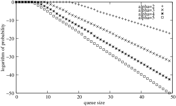
Figure 3 demonstrates the tradeoff between the queue size and the number of active middle-stage nodes. For this instance, the router is again . The link rate of the interconnect is set to . The traffic is fully loaded for each of the inputs and outputs. If we keep all nodes in the middle stage active, we can see from the bottom curve of Figure 3 that the queue size is the smallest. However, this option is also the most energy consuming as all 80 middle-stage nodes are kept active. For the other extreme, we can activate 40 middle-stage nodes, which is the most energy efficient. However, we can see from the bottom curve of Figure 3 that the queue size is the smallest. The curves in between correspond to the intermediate cases in which the number of active middle-stage nodes are 50, 60 and 70.

VI Conclusion
In this paper we revisit the Load-Balanced Router architecture, motivated by its potential of delivering energy proportionality for routers. We offer a detailed analysis on the queue lengths and packet delays under a simple random routing algorithm which is robust against all admissible traffic. This allows us to observe a trade off between performances such as queue size against energy consumption.
Our paper does not focus on algorithms that optimize the number of active middle-stage nodes. We give a very simple argument for which the size of the active middle stage is proportional to the maximum traffic load over all inputs and outputs. It is an intriguing open question to see how one could make sure that the size of the active middle stage is proportional to the traffic average over all input, not to the maximum.
References
- [1] Routing telecom and data centers toward efficient energy use. In Proceedings of the Vision and Roadmap Workshop, U.S. Department of Energy, October 2008.
- [2] S. Antonakopoulos, S. Fortune, A. Francini, T. Klein, R. McLellan, D. Nielson, and L. Zhang. Personal communication, 2011.
- [3] N. Bansal, T. Kimbrel, and K. Pruhs. Speed scaling to manage energy and temperature. Journal of the ACM, 54(1), 2007.
- [4] J. Y. L. Boudec and P. Thiran. Network Calculus. Springer Verlag, http://ica1www.epfl.ch/ PS_files/NetCal.htm, 2004.
- [5] H.-L. Chan, W.-T. Chan, T. W. Lam, L.-K. Lee, K.-S. Mak, and P. W. H. Wong. Energy efficient online deadline scheduling. In Proceedings of ACM-SIAM SODA, pages 795–804, 2007.
- [6] C. Chang, D. Lee, and Y. Jou. Load balanced Birkhoff-von Neumann switches, part I: one-stage buffering. In IEEE HPSR ’01, Dallas, TX, 2001.
- [7] C. Chang, D. Lee, and C. Lien. Load balanced Birkhoff-von Neumann switches, part II: multi-stage buffering. Computer Comm., 25:623 – 634, 2002.
- [8] C. Chang, D. Lee, and Y. Shih. Mailbox switch: a scalable two-stage switch architecture for conflict resolution of ordered packets. In Proceedings of IEEE INFOCOM 2004, Hong Kong, 2004.
- [9] C. Chang, D. Lee, and C. Yue. Providing guaranteed rate services in the load balanced Birkhoff-von Neumann switches. In Proceedings of IEEE INFOCOM 2003, San Francisco, CA, 2003.
- [10] R. L. Cruz. A calculus for network delay, Part I: Network elements in isolation. IEEE Transactions on Information Theory, 37(1):114 – 131, 1991.
- [11] R. L. Cruz. A calculus for network delay, Part II: Network analysis. IEEE Transactions on Information Theory, 37(1):132 – 141, 1991.
- [12] A. Francini, S. Fortune, T. Klein, and M. Ricca. Energy profiling of network equipment for rate adaptation technologies. Internal Technical Documents, Alcatel-Lucent, 2011.
- [13] A. Francini and D. Stiliadis. Energy efficiency with rate adaptation. In Proc. of IEEE HPSR, 2010. http://ect.bell-labs.com/who/francini/ra9.pdf.
- [14] M. Garrett. Powering down. Commun. ACM, 51(9):42–46, 2008.
- [15] N. M. I. Keslassy, S.T. Chuang. A load-balanced switch with an arbitrary number of linecards. In Proceedings of IEEE INFOCOM 2004, Hong Kong, 2004.
- [16] S. Irani and K. Pruhs. Algorithmic problems in power management. SIGACT News, 36(2):63–76, 2005.
- [17] S. Irani, S. K. Shukla, and R. Gupta. Algorithms for power savings. ACM Transactions on Algorithms, 3(4), 2007.
- [18] S. Irani, S. K. Shukla, and R. K. Gupta. Online strategies for dynamic power management in systems with multiple power-saving states. ACM Trans. Embedded Comput. Syst., 2(3):325–346, 2003.
- [19] Y. Jiang. A basic stochastic network calculus. In Proceedings of ACM SIGCOMM ’06, pages 123 – 134, New York, NY, 2006.
- [20] Y. Jiang and P. J. Emstad. Analysis of stochastic service guarantees in communication networks: A server model. In In Proc. of the International Workshop on Quality of Service (IWQoS 2005, pages 233–245, 2005.
- [21] I. Keslassy, S.-T. Chuang, D. M. K. Yu, M. Horowitz, and O. Solgaard. Scaling internet routers using optics. In Proceedings of ACM SIGCOMM ’03, Karlsruhe, Germany, 2003.
- [22] I. Keslassy and N. McKeown. Maintaining packet order in two-stage switches. In Proceedings of IEEE INFOCOM 2002, New York, NY, June 2002.
- [23] M. Li, B. J. Liu, and F. F. Yao. Min-energy voltage allocation for tree-structured tasks. In Proceedings of COCOON, pages 283–296, 2005.
- [24] N. W. McKeown, V. Anantharam, and J. Walrand. Achieving 100% throughput in an input-queued switch. In Proceedings of IEEE INFOCOM ’96, pages 296 – 302, San Francisco, CA, March 1996.
- [25] S. Nedevschi, L. Popa, G. Iannaccone, S. Ratnasamy, and D. Wetherall. Reducing network energy consumption via sleeping and rate-adaptation. In Proceedings of NSDI, pages 323–336, 2008.
- [26] M. Roughan, A. Greenber, C. Kalmanek, M. Rumescwicz, J. Yates, and Y. Zhang. Experience in measuring internet backbone traffic variability. In Proc. ACM SIGCOMM IMW, pages 91 – 92, 2002.
- [27] C. Scheideler. Probabilistic Methods for Coordination Problems. Habilitation thesis, Paderborn University, 2000.
- [28] L. G. Valiant. A scheme for fast parallel communication. SIAM J. Comput., 11(2):350 – 361, 1982.
- [29] F. F. Yao, A. Demers, and S. Shenker. A scheduling model for reduced CPU energy. In Proceedings of IEEE FOCS, pages 374–382, 1995.