Catching the fish – Constraining stellar parameters for TX Psc using spectro-interferometric observationsThanks: Based on observations made with ESO telescopes at Paranal Observatory under program IDs 74.D-0601, 60.A-9224, 77.C-0440, 60.A-9006, 78.D-0112, 84.D-0805
Abstract
Context. Stellar parameter determination is a challenging task when dealing with galactic giant stars. The combination of different investigation techniques has proven to be a promising approach. We analyse archive spectra obtained with the Short-Wavelength-Spectrometer (SWS) onboard of ISO, and new interferometric observations from the Very Large Telescope MID-infrared Interferometric instrument (VLTI/MIDI) of a very well studied carbon-rich giant: TX Psc.
Aims. The aim of this work is to determine stellar parameters using spectroscopy and interferometry. The observations are used to constrain the model atmosphere, and eventually the stellar evolutionary model in the region where the tracks map the beginning of the carbon star sequence.
Methods. Two different approaches are used to determine stellar parameters: (i) the ‘classic’ interferometric approach where the effective temperature is fixed by using the angular diameter in the -band (from interferometry) and the apparent bolometric magnitude; (ii) parameters are obtained by fitting a grid of state-of-the-art hydrostatic models to spectroscopic and interferometric observations.
Results. We find a good agreement between the parameters of the two methods. The effective temperature and luminosity clearly place TX Psc in the carbon-rich AGB star domain in the H-R-diagram. Current evolutionary tracks suggest that TX Psc became a C-star just recently, which means that the star is still in a ‘quiet’ phase compared to the subsequent strong-wind regime. This is in agreement with the C/O ratio being only slightly larger than 1.
Key Words.
Stars: AGB and post-AGB - Stars: atmospheres - Stars: carbon - Stars: fundamental parameters - Techniques: interferometric - Techniques: spectroscopic1 Introduction
The asymptotic giant branch (AGB) is the late evolutionary stage of low- to intermediate- mass
stars ( ). On the early-AGB the carbon-to-oxygen-ratio is smaller than one. After
several thermal pulses, the atmospheres of objects with masses between will
very likely turn from oxygen-rich into carbon-rich because of the third dredge-up (Iben & Renzini 1983).
Good estimates of stellar parameters are needed for a profound understanding of the evolution of
this stage. Their determination is a challenging task because of the complexity of the atmospheres
of these objects. It is demonstrated that the combined use of spectroscopic and
interferometric observing techniques can efficiently help to ascertain stellar parameters
(Wittkowski et al. 2001; Wittkowski et al. 2008; Wittkowski et al. 2011; Neilson & Lester 2008; Paladini et al. 2011; Sacuto et al. 2011a; Martí-Vidal et al. 2011, e.g.).
At the same time these observations provide constraints for existing model atmospheres:
e.g. COMARCS (Aringer et al. 2009), Höfner et al. (2003), PHOENIX (Hauschildt et al. 1999), ATLAS (Kurucz 1993, e.g.),
CODEX (Ireland et al. 2008; Ireland et al. 2011).
TX Psc is one of the brightest and closest carbon-rich AGB stars. It is listed as an irregular variable in
the General Catalogue of Variable stars (Samus et al. 2009) with a mean brightness of
5 mag and a peak-to-peak amplitude of 0.4 mag in the -band (Jorissen et al. 2011). Distance
estimates range from 275 to 315 pc (van Leeuwen 2007; Claussen et al. 1987; Bergeat & Chevallier 2005). Different ISO/SWS
spectra of TX Psc (Jørgensen et al. 2000; Gautschy-Loidl et al. 2004) show that there is a difference in the 3 m
feature between 1996 and 1997. With the help of plane-parallel, hydrostatic models
Jørgensen et al. (2000) interpret this difference as a change in temperature of 100 K. The
photometry and spectra were successfully modeled by Gautschy-Loidl et al. (2004) with dust-free dynamical
models that reproduce the region between m. They claim that the region between
m is affected almost solely by CS.
The authors suggest that observations from m show the deep
photosphere, while the expected absorption of HCN and
C2H2 originating from the higher layers is not observed. As this object is almost (carbon)
dust-free we may infer it became a carbon star quite recently. Therefore, this star is a perfect candidate
to constrain the region where the transition from oxygen- to carbon-rich occurs.
In this work we present a study of the atmosphere and a stellar parameter determination for TX Psc. We
combine spectro-interferometric observations of VLTI/MIDI and spectroscopic observations from ISO/SWS
and compare them to geometric, hydrostatic, and evolutionary models.
A description of observations and data reduction is given in
Sect. 2. Models and approaches to derive synthetic observables are
presented in Sect. 3. The stellar parameters are derived in Sect. 4
and compared to state-of-the-art evolutionary tracks in Sect. 5. A summary of the results is
given in Sect. 6.
2 Observations and Data Reduction
Sections 2.1 and 2.2 discuss the interferometric and spectroscopic observations obtained with VLTI/MIDI and ISO/SWS, respectively. Section 2.3 discusses possible cycle-to-cycle and intra-cycle variability of the data.
2.1 MIDI visibilities and spectra

TX Pscwas observed in 2004 with the 8.2 m Unit Telescopes and in 2005, 2006 and 2011 with
the 1.8 m Auxiliary Telescopes of the Very Large Telescope Interferometer MIDI (Leinert et al. 2003). MIDI
covers the -band and provides spectrally dispersed visibilities, differential phases and fluxes
(resolution for observations in 2004, for observations in 2005,
2006 and 2011).
The journal of available MIDI observations is given in Table 1 (electronic version only).
The -coverage is plotted in Fig. 1.
\onltab1
| # | Object | Date/Time | Configuration | Proj.Base | Proj.Angle | Obs. seeing | Airmass |
| [m] | [∘] | [″] | |||||
| 1 | TXPSC | 2006-08-28 02:50 | E0-G0 | 9.4 | 81 | 1.41 | 1.718 |
| 2 | TXPSC a aa a aa Calibrated spectrum available | 2006-10-19 00:19 | E0-G0 | 11.9 | 70 | 1.387 | |
| HD48915 | 2006-10-19 08:26 | … | … | … | 0.57 | 1.325 | |
| 3 | TXPSC | 2006-10-18 05:46 | E0-G0 | 13.2 | 66 | 0.89 | 1.659 |
| HD48915 | 2006-10-18 06:57 | … | … | … | 0.87 | 1.278 | |
| 4 | TXPSC | 2005-06-29 08:55 | E0-G0 | 13.7 | 82 | 0.54 | 1.238 |
| 5 | TXPSC | 2010-09-07 04:13 | E0-G0 | 14.4 | 73 | 0.93 | 1.194 |
| 6 | TXPSC | 2006-08-28 05:48 | E0-G0 | 15.6 | 73 | 1.30 | 1.136 |
| 7 | TXPSC | 2009-11-15 02:18 | E0-G0 | 15.7 | 72 | 1.26 | 1.225 |
| 8 | TXPSC a aa a aa Calibrated spectrum available | 2006-10-18 03:18 | E0-G0 | 16.0 | 73 | 1.00 | 1.149 |
| HD48915 | 2006-10-18 06:57 | … | … | … | 0.87 | 1.278 | |
| 9 | TXPSC | 2006-09-20 02:28 | D0-G0 | 25.1 | 71 | 1.21 | 1.327 |
| 10 | TXPSC | 2006-09-20 03:23 | D0-G0 | 29.0 | 73 | 1.90 | 1.189 |
| 11 | TXPSC | 2006-10-16 02:12 | H0-G0 | 30.5 | 73 | 0.67 | 1.150 |
| 12 | TXPSC | 2009-11-16 02:13 | H0-G0 | 31.0 | 72 | 0.95 | 1.219 |
| 13 | TXPSC | 2006-09-20 05:47 | D0-G0 | 31.6 | 72 | 1.64 | 1.201 |
| HD20720 | 2006-09-20 09:48 | … | … | … | 0.89 | 1.095 | |
| 14 | TXPSC | 2009-11-16 01:20 | H0-G0 | 32.0 | 73 | 1.36 | 1.146 |
| 15 | TXPSC | 2006-09-21 01:48 | K0-G0 | 44.0 | 68 | 1.01 | 1.489 |
| 16 | TXPSC a aa a aa Calibrated spectrum available | 2006-09-21 03:32 | K0-G0 | 59.3 | 73 | 1.02 | 1.169 |
| HD48915 | 2006-09-21 08:36 | … | … | … | 1.51 | 1.309 | |
| 17 | TXPSC | 2006-09-17 04:20 | A0-G0 | 62.0 | 73 | 1.36 | 1.140 |
| 18 | TXPSC a aa a aa Calibrated spectrum available | 2006-09-21 05:55 | K0-G0 | 62.6 | 72 | 1.39 | 1.225 |
| HD48915 | 2006-09-21 08:36 | … | … | … | 1.51 | 1.309 | |
| 19 | TXPSC | 2008-09-27 04:45 | G1-D0 | 63.6 | 133 | 1.00 | 1.155 |
| 20 | TXPSC | 2006-08-17 07:00 | A0-G0 | 63.8 | 73 | 0.39 | 1.137 |
| HD224935 | 2006-08-17 07:23 | … | … | … | 0.43 | 1.060 | |
| 21 | TXPSC | 2004-10-30 03:28 | UT2-UT4 | 84.3 | 80 | 0.78 | 1.244 |
| HD49161 | 2004-10-30 09:19 | … | … | … | 0.72 | 1.196 | |
| 22 | TXPSC | 2006-08-16 07:06 | A0-G1 | 87.1 | 113 | 0.85 | 1.137 |
| HD18884 | 2006-08-16 07:57 | … | … | … | 0.81 | 1.353 | |
| 23 | TXPSC | 2006-08-15 06:20 | A0-G1 | 90.3 | 113 | 0.88 | 1.145 |
| 24 | TXPSC | 2011-09-21 05:39 | I1-A1 | 104.0 | 84 | 1.03 | 1.186 |
| 25 | TXPSC | 2011-10-05 04:21 | K0-A1 | 129.0 | 67 | 0.57 | 1.158 |
| 26 | TXPSC a aa a aa Calibrated spectrum available | 2011-10-02 05:44 | A1-J3 | 140.0 | 46 | 1.02 | 1.305 |
| HD45348 | 2011-10-02 06:42 | … | … | … | 0.88 | 1.512 |
Data are reduced using MIA+EWS 1.7.122
2
http://www.strw.leidenuniv.nl/jaffe/ews/MIA+EWS-
Manual/index.html
(Jaffe 2004; Ratzka 2005; Leinert et al. 2004).
Observations are not used if one or more of the selection criteria discussed in Klotz et al. (2012a) are
violated (observations that are not boldfaced in Table 1).
Uniform-disk angular diameters and IRAS 12 m flux of the calibrator targets are given in
Table 2 (electronic version only).
\onltab2
| HD | Name | Sp. T.
a
aa
a
aa
http://www.eso.org/observing/dfo/quality/MIDI/qc/
calibrators_obs.html |
a
aa
a
aa
http://www.eso.org/observing/dfo/quality/MIDI/qc/
calibrators_obs.html |
b bb b bb http://simbad.u-strasbg.fr/simbad/ |
|---|---|---|---|---|
| [Jy] | [mas] | |||
| HD 48915 | Sirius | A1 | 143.13 | 6.08 |
| HD 20720 | 04 Eri | M3/M4 | 162.76 | 10.140.04 |
| HD 224935 | YY Psc | M3 | 86.95 | 7.250.03 |
| HD 49161 | 17 Mon | K4 | 10.45 | 2.440.01 |
| HD 18884 | Cet | M1.5 | 234.73 | 12.280.05 |
| HD 45348 | Canopus | F0 | 154.83 | 6.870.03 |
As only one suitable calibrator is available per observation, a standard multiplicative
error of 10% is assumed for the calibrated visibilities (Chesneau 2007) . Some calibrated visibilities at baselines shorter than
30 m are significantly noisier and sometimes larger than unity after 11.5 m. Therefore,
in the following, spectro-interferometric observations are considered only for wavelengths shorter than
11.5 m.
For the calibrated spectra additional selection criteria are applied (Chesneau 2007):
(i) the airmass difference between science and calibrator observations is ,
(ii) the spectral type of the calibrator is not later than M0. Considering these criteria, five spectra are derived
(flagged with ‘a’ in Table 1).
TX Psc is almost unresolved for baselines shorter than 32 m. Therefore, we
expect that the star is unresolved by the single-dish UTs. Thus, most of the mid-infrared (mid-IR) flux is located
within the field-of-view (FoV) of the UTs and consequently also in the FoV of the ATs and ISO, which
makes the spectra fully comparable to each other.
2.2 ISO spectra
Three spectra of TX Psc were observed with the Short-Wavelength-Spectrometer (de Graauw et al. 1996, SWS,) onboard of ISO (Sloan et al. 2003; Jørgensen et al. 2000). Two spectra have a resolution of and range from m. The other spectrum ranges from m and has a resolution of which has been binned to the resolution of the other spectra. For the ISO spectra a multiplicative error of % is assumed from 2.38-4.05 m and % afterwards (Sloan et al. 2003).
2.3 Interferometric and spectroscopic variability
In the left panel of
Fig. 2 the calibrated MIDI spectra are overplotted to the ISO/SWS spectra. The flux level of the MIDI
observations is the same (within the error bars) as the ISO/SWS spectra taken at 1996 Nov 26 and 1997 Dec 11.
This suggests that no significant cycle-to-cycle variation is expected in the mid-IR.
The right plot of Fig. 2 shows part of the lightcurve of TX Psc in taken from AAVSO. The spectra
from 1996 Nov 26/1997 Dec 11 were observed at a ’local’ visual maximum/minimum, respectively.
In the following we will use these two spectra to derive the parameters
of the star at different phases. As we do not have any information on the magnitude of the spectrum from 1997
May 24, this spectrum is not used in the subsequent sections. Additionally, the phase for all the MIDI observations
is unknown. However, AAVSO visual estimates from one specific observer revealed that none of the MIDI
observations were taken at visual minima or maxima.
Simulations with dust-free model atmospheres show that the effect of pulsation on
the -band UD-radius is smaller than 0.1 mas at 1 kpc (Paladini et al. 2009). For a star at the distance of TX Psc this
would be 0.3 mas. This value is beyond the limit of resolution of MIDI. Therefore, we do not expect any
observed intra-cycle variability effect that is larger than the errors. This allows to combine all calibrated
visibilities for the further analysis.


3 Model description
In the following we present the different classes of models and the derivation of synthetic observables that will be compared to observations in Sect. 4.
3.1 Hydrostatic models
Observed spectra and visibilities are compared to the grid of spherical hydrostatic model atmospheres and spectra of
Aringer et al. (2009). These models are computed with COMARCS and are generated assuming hydrostatic local thermal and chemical equilibrium.
The molecular and atomic opacities are treated in the opacity sampling (OS) approximation. The parameters that
characterize a model are: effective temperature Teff, metallicity , surface gravity , mass ,
and carbon to oxygen ratio C/O.
For this work we limit the sample to
models having solar metallicity as the effect of metallicity is expected to be small for low-resolution
spectroscopy. Additionally, there is no indication for largely non-solar metallicity from other properties
of this star.
The spectra cover the following parameters: K with steps of
100 K; ; logcm s; ; C/O. In order to get precise estimates of Teff, additional model atmospheres were
produced resulting in a grid spacing of T=10 K. All the main molecular
opacities typical for C-stars were included: CO (Goorvitch & Chackerian 1994), C2
(Querci et al. 1974), HCN (Harris et al. 2006), CN (Jørgensen 1997) in the form of line lists, while C2H2 and
C3 (Jorgensen et al. 1989) as OS data. CS is not included due to the lack of line lists and OS data.
Synthetic spectra with a resolution of 18 000 are
computed in the wavelength range m. The spectra are convolved in order to get the same
resolution as the observed data.
Among the output of the spherical radiative transfer code COMA is the monochromatic spatial intensity profile.
This profile is used to calculate a synthetic visibility profile in the mid-IR for a subset of the models in the
grid. A detailed
description of the computation of the visibility profiles is given in Paladini et al. (2009).
3.2 Evolutionary tracks
The luminosity and effective temperature that are determined from hydrostatic models are compared to thermally-pulsing (TP) AGB evolutionary tracks from Marigo et al. (in prep). We selected TP-AGB sequences with an initial scaled-solar chemical composition (, ), where and denote the mass fractions of metals and helium, respectively. TP-AGB evolutionary calculations are carried out from the first thermal pulse - extracted from the PARSEC database of stellar models (Bressan et al. 2012) - to the complete ejection of the envelope due to stellar winds. The TP-AGB tracks are based on numerical integrations of complete envelope models in which, for the first time, molecular chemistry and gas opacities are computed on-the-fly with the ÆSOPUS code (Marigo & Aringer 2009). This guarantees a full consistency of the envelope structure with the surface chemical abundances that may significantly vary due to the third dredge-up episodes and hot-bottom burning. The transition from C/O to C/O is followed accurately, in particular in the narrow range from C/O , where an abrupt change in the molecular chemistry and opacity is expected to occur (Marigo & Aringer 2009, see figures 11 and 16 in). This point is particularly relevant in the context of the present work, as TX Psc is found to have a surface C/O slightly above unity.
4 Stellar parameter determination
Stellar parameters for TX Psc were determined by a number of authors. A summary is given in Table 3.
| Reference | log | Mass | C/O | d | |||
|---|---|---|---|---|---|---|---|
| [K] | [] | [mas] | [m] | [pc] | |||
| Lasker et al. (1973) | 9.00 | 0.66 | |||||
| de Vegt (1974) | 8.00 | 0.71 | |||||
| Dunham et al. (1975) | 10.20 | 0.69 | |||||
| Lambert et al. (1986) | 3 030 | 0.0 | 1.03 | ||||
| Claussen et al. (1987) | 280 | ||||||
| Quirrenbach et al. (1994) | 2 805 | 11.20 | 0.7-0.8 | ||||
| Richichi et al. (1995) | 8.38 | 0.55-3.60 | |||||
| Dyck et al. (1996) | 2 921 | 11.20 | 2.2 | ||||
| Jørgensen et al. (2000) | 3 000 | -0.5 | 1.02 | ||||
| Ohnaka et al. (2000) | 3 000 | 1.07 | |||||
| 3 100 | 1.17 | ||||||
| Bergeat et al. (2001) | 3 115 | ||||||
| Harris et al. (2003) | 3 050 | 0.0 | 1.02 | ||||
| Gautschy-Loidl et al. (2004) | 3 200 | -0.3 | 1 | 1.10 | |||
| Bergeat & Chevallier (2005) | 3 125 | 315 | |||||
| Ragland et al. (2006) | 9.89 | 1.65 | |||||
| van Leeuwen (2007) | 275 |
In the following two different approaches will be used to determine the stellar parameters of TX Psc: (i) in Sect. 4.1 we use the ‘classical approach’ of interferometrists where spectro-interferometric observations are used to determine the effective temperature ; (ii) in Sect. 4.2 we follow the approach of Paladini et al. (2011, P11 hereafter) where spectroscopic/interferometric measurements are compared to hydrostatic models to determine and C/O ratio and to constrain mass and log .
4.1 Approach 1: Geometric models
Interferometry is a powerful tool for constraining the morphology and size
of stars and their environments.
A deviation from spherical symmetry for the circumstellar environment of TX Psc was detected
by several authors at different spatial scales and wavelengths
(e.g. Cruzalèbes et al. 1998; Ragland et al. 2006; Sacuto et al. 2011b; Jorissen et al. 2011, Hron et al in prep.).
Clearly, the circumstellar environment of TX Psc is very complex and most likely unrelated effects shape the
morphology in different regions, resulting in a large variety of structures. To study the geometry of the innermost
region of the star in the -band, the geometrical model fitting tool GEM-FIND (Klotz et al. 2012b) was used to fit
the MIDI interferometric observations of TX Psc.
A spherical UD-model is able to reproduce the calibrated visibilities, i.e. TX Psc can be assumed to be
spherically symmetric in the mid-IR at spatial scales probed by
our MIDI observations. The reason why the asymmetrical structures detected by other works are not observed is that
they were either detected at
distances outside the FoV of MIDI or at smaller spatial scales beyond
the detection limit of MIDI. This is supported by the differential phase measurements
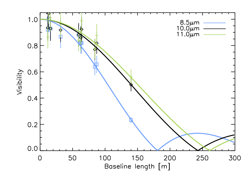
of MIDI, which do not show any deviation from zero. The calibrated visibilities are plotted together with
the best-fitting UD-model in the
left panel of Fig. 3 for three different wavelenghts.
The right panel of Fig. 3 shows the wavelength dispersed diameter calculated with the UD-model
(dark grey shaded area). The star appears larger between 8 and 9 m. According to Gautschy-Loidl et al. (2004)
CS is affecting this wavelength range. Because of this molecular contamination, this region is omitted
and a mean angular diameter of mas
is calculated by averaging the diameter from 9-11.5 m.

4.1.1 Effective temperature
The temperature can be determined using the apparent bolometric magnitude
and the angular Rosseland diameter .
The apparent bolometric magnitude mag was derived by F. Kerschbaum
by fitting a combination of blackbodies to near-IR and IRAS data44
4
Method described in
Kerschbaum & Hron (1996a) and references therein; near-IR data from the IRAS catalogue and Fouque et al. (1992)..
Various definitions for the radius can be found in literature (Baschek et al. 1991; Scholz 2003, c.f. reviews by), where the most
commonly used radius in atmospheric modeling is the Rosseland radius. It is defined by the distance between the
center of the star and the layer having Rosseland optical depth . This radius, however,
is not an observable quantity and observed radii have to be converted
by using model considerations.
In the following we will derive this conversion factor for hydrostatic C-stars by using a subset
of the hydrostatic models in the grid of Aringer et al. (2009) to derive a mean
UD-radius in the mid-IR ( m).
This mean UD-radius is plotted versus the Rosseland radius of the corresponding hydrostatic model in Fig. 4.
There is a clear correlation between the two radii, yielding
| (1) |

This implies that for a hydrostatic C-star the Rosseland radius can be approximated by
the mid-IR UD-radius if the derived correction factor of 0.95 is applied.
Applying this correction factor yields an angular Rosseland diameter mas. Together with the bolometric
magnitude the distance-independent effective temperature can be derived.
Using the three different distance estimates that are available for TX Psc (see Table 3) a linear radius and
luminosity can be calculated.
Table 4 lists the derived and calculated stellar parameters of approach 1. Errors on the temperature
are determined by using
the errors on and by assuming an arbitrary error of for mbol that accounts for the
stellar variability and the fitting error. These values are in agreement with
those given in literature (see Table 3).
| pc] | [mas] | [mas] | [K] | [] | [] |
|---|---|---|---|---|---|
| 275 | 10.510.70 | 9.99 | 3127 | 294 | 7 406 |
| 280 | 10.510.70 | 9.99 | 3127 | 299 | 7 678 |
| 315 | 10.510.70 | 9.99 | 3127 | 337 | 9 717 |
4.2 Approach 2: Hydrostatic models
The short wavelength part of the ISO spectrum of TX Psc is dominated by the 3 m feature which has
contributions from HCN and C2H2.
The 5 m feature, on the other hand, is due to C3 and the fundamental band of CO. The region from 7 to
8 m is dominated by HCN and C2H2 and according to Gautschy-Loidl et al. (2004) the region from 8 to 9 m
is affected by CS opacity. The low variability in the -band
( mag) justifies the use of
hydrostatic models in the near- as well as mid-IR.
Additionally, hydrostatic models are able to reproduce large parts of the overall ISO
as well as MIDI spectra. This indicates that the circumstellar environment of TX Psc
is optically thin and contains almost no dust.
In Sect. 4.2.1 and 4.2.2 low-resolution spectroscopic observations are compared with synthetic
spectra of hydrostatic models to fix the fundamental stellar parameters C/O ratio and . The
overall energy distribution as well as the bands of the molecules that are present from 2.3-6 m put strong
constraints on these parameters (Jørgensen et al. 2000; Loidl et al. 2001; P11).
Low resolution spectroscopy does not allow to ascertain mass and log (Fig. 6-10 in P11). To determine
these parameters Sect. 4.2.3 follows the approach described in P11: spectro-interferometric observations are
compared to models of fixed and C/O ratio but varying log and mass.
4.2.1 C/O ratio
Jørgensen et al. (2000) found the ratio between the 3 m feature (HCN and C2H2) and the 5.1 m feature (CO and C3) to be a sensitive measure of the C/O ratio. In order to be independent of distance each model spectrum is normalized to the ISO flux at 2.9 m (Aringer et al. 2009, local minimum of molecular absorption,). A test is applied between 2.9 - 6.0 m to compare the observed ISO spectra (1996 Nov 26 and 1997 Dec 11) to the models. For both ISO spectra we find that the best solution is obtained with a C/O ratio of 1.05. Considering all solutions lying within the 68% confidence level a C/O ratio of 1.1 can be defined as an upper limit. Due to the coarse grid spacing for C/O this value is not a strict upper limit and no lower limit can be assigned. Figs. 5 and 6 show the ISO/SWS spectrum plotted together with models of different temperatures and C/O ratios. The upper panels draw the region around the 3 m and 5.1 m feature to a larger scale. These plots demonstrate that a synthetic spectrum with a C/O ratio larger or equal 1.4 is not able to reproduce the observations, because it over-evaluates the depth of the 5.1 m feature. This finding is consistent with the C/O ratios given in literature (see Table 3).


4.2.2 Effective temperature
We expect the 3 m feature to be a good temperature indicator for hydrostatic stars (P11). Consequently, in order to find the best
temperature for TX Psc, a test is used to compare the observed ISO spectra and the model spectra between 2.9 -
3.6 m. Only model spectra lying within the confidence level of C/O (1.05, 1.1; see Sect. 4.2.1) are used
for this test.
The large grid of models allows to determine Teff very precisely. All solutions lying within the 68% confidence
level have a temperature of 3 080 / 3 170 K for the visual minimum/maximum, respectively. The upper
left panel of Figs. 5 and 6 show that models with higher/lower temperatures do not reproduce the depth
of the 3 m feature.
The temperature derived with approach 1 in Sect. 4.1.1 is within the errors of the temperature that is
derived here for the visual minimum and maximum.
We confirm the finding of Jørgensen et al. (2000) that the difference in the two ISO spectra can be explained by a temperature
change. The lightcurve suggests that this difference is due to variability effects, but time-series spectroscopy is needed to
confirm this finding.
4.2.3 Surface gravity and mass
Interferometric observations are compared to synthetic visibilities of hydrostatic models of varying log g and mass
using a test.
All synthetic visibilities are computed for the best-fitting values of Teff and C/O-ratio from
Sects. 4.2.1 and 4.2.2. Synthetic visibilities are derived at
3 different distances: 275 pc, 280 pc, 315 pc
(van Leeuwen 2007; Claussen et al. 1987; Bergeat & Chevallier 2005, respectively). In Fig. 7 the wavelength-dispersed calibrated visibilities are plotted together with the
synthetic visibilities of the best-fitting models. The region between 8 - 9 m is not considered in the fitting, as the
hydrostatic models do not include the CS opacity data.
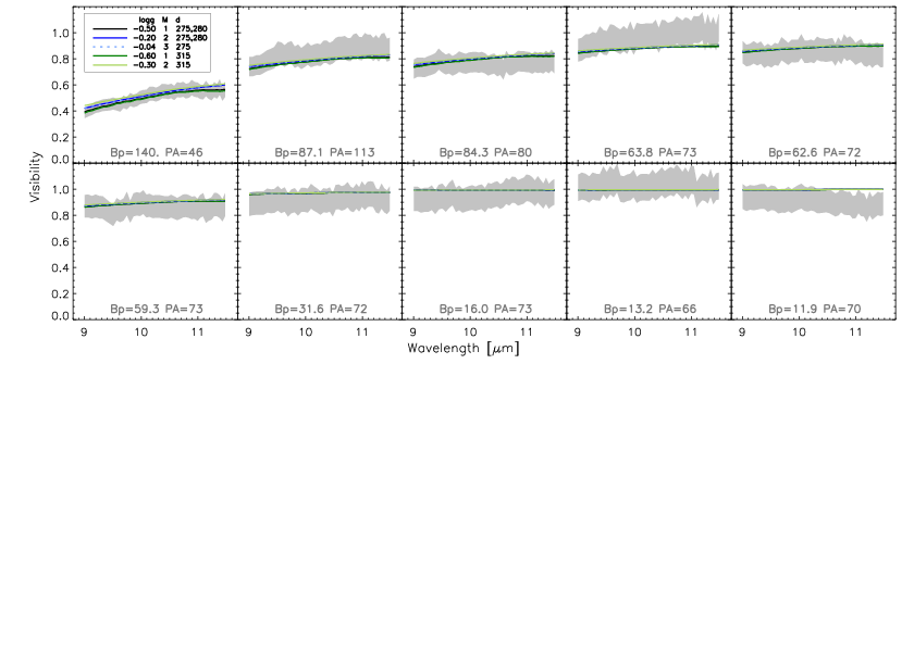
The middle block of Table 5 gives the best-fitting stellar parameters for a given distance that were determined using
approach 2.
It is clear from the table and from Fig. 7 that, given the error bars on the visibilities, there
is a degeneracy between log and mass.
As the distance defines the level of visibility, there is also a degeneracy between distance and log .
From current TP-AGB evolutionary calculations (e.g. Karakas et al. 2002; Marigo & Girardi 2007, Marigo et
al. in prep.) we expect that a TP-AGB star with solar metallicity does not make the
transition to the C-rich domain.
This suggests that the log values in Table 5 found for are the more reliable ones.
But, considering the degeneracy
and the limited mass sampling ( ) in the grid, also models with higher masses
would reproduce the observed visibilities. To support this statement, one additional model with 3 is calculated and
overplotted in Fig. 7 as dashed line. The models are almost indistinguishable.
The right part of Table 5 gives stellar parameters that are calculated from the derived log , mass
and effective temperature.
The luminosities are significantly larger than the used by Gautschy-Loidl et al. (2004), but
comparable to derived by Claussen et al. (1987). The luminosities and radii are also in perfect agreement
with the ones determined with approach 1 (see Sect. 4.1).
4.2.4 Photometric constraints on the best model
The best fitting hydrostatic models of visual minimum/maximum (model with lowest in Table 5) are overplotted to the ISO and MIDI spectra as well as to photometric measurements in Fig. 8. Photometric measurements from Johnson et al. (1966), Mendoza V. & Johnson (1965) and Catchpole et al. (1979) were observed with the Johnson filter system. Zero points to convert these measurements from magnitudes to Jansky are taken from Cox (2000). These zero points are also used to convert observations from Bergeat et al. (1976) and Bergeat & Lunel (1980) as the authors claim that their filter system is similar to the Johnson filter system. Zero points for 2MASS photometry (Cutri et al. 2003) are given in Cohen et al. (2003). Olofsson et al. (1993) and Kerschbaum et al. (1996b) used the ESO filter system. Zero points are taken from Le Bertre (1988) and Wamsteker (1981). Noguchi et al. (1981) used their own filter system and corresponding zero points are given in their paper.
| C/O | log | ||||||||
|---|---|---|---|---|---|---|---|---|---|
| pc] | [K] | [K] | [] | [] | [] | [] | |||
| 275 | 3080 | 3170 | 1.05 | -0.5 | 1 | 0.50 | 295 | 7019 | 7876 |
| -0.2 | 2 | 0.50 | 295 | 7019 | 7876 | ||||
| 280 | 3080 | 3170 | 1.05 | -0.5 | 1 | 0.48 | 295 | 7019 | 7876 |
| -0.2 | 2 | 0.53 | 295 | 7019 | 7876 | ||||
| 315 | 3080 | 3170 | 1.05 | -0.6 | 1 | 0.49 | 331 | 8836 | 9915 |
| -0.3 | 2 | 0.53 | 331 | 8836 | 9915 |

5 Comparison with evolutionary tracks
We follow the approach described in P11 and compare the stellar parameters with new
evolutionary tracks of thermally pulsing AGB stars (Marigo et al., in prep).
Figure 9 depicts evolutionary tracks in the region of AGB stars in the H-R diagram.
Overplotted are the determined luminosity and temperature for
TX Psc for the two approaches.
Only the best-fitting luminosity (see Table
5) at d=280 pc is plotted for TX Psc. Errors for the luminosity are assumed to lie in the order of 40%
(uncertainty on the given distance measurement).
We note an encouraging agreement between the observed location of TX Psc in the H-R
diagram and the predicted ranges of luminosity and effective temperature for a carbon-rich star with
solar-metallicity and C/O within a narrow interval (i.e. 1C/O1.1). As we see in
Fig. 9, the TP-AGB evolutionary tracks in the C-rich regime
extend to much
lower effective temperatures than the derived values for TX Psc. This cooling is mainly driven by the increase of the
C/O ratio after each dredge-up episode, as well as by the progressive strengthening of the mass-loss efficiency.
The relatively warm effective temperature of TX Psc suggests that this star is observed close after the transition into
the C-star domain, in an early ‘quiet’ stage in which the strong wind has not yet developed. This
picture is nicely supported by the observational findings already discussed in the previous sections.
It is visible from the evolutionary tracks that an AGB star with solar metallicity will turn into a carbon-rich AGB star
only for masses around 2 and higher. Also, the position of TX Psc in Fig. 9
suggests that the mass lies between 2 and 3 . This is not in agreement with the best fitting models
having 1 (Sect. 4.2.3), but in good agreement with the models having 2 .
6 Conclusion
In this work we determined stellar parameters for TX Psc by comparing observations to geometric models (Klotz et al. 2012b),
state-of-the-art hydrostatic model atmospheres (Aringer et al. 2009) and evolutionary models (Marigo et al. in prep.).
Two different approaches were used to fix the parameters:
A1. Spectro-interferometric observations
were used to determine a wavelength-dispersed uniform disk diameter. A correction factor for hydrostatic
C-stars was derived from hydrostatic models to convert the UD diameter to the Rosseland radius, which was then used
to determine the effective temperature .
A2. Spectroscopic measurements were compared
to synthetic spectra from hydrostatic models to determine and C/O ratio.
The mass and log were constrained by comparing
spectro-interferometric observations with synthetic visibility profiles from hydrostatic models.
The main advantage of approach 1 is the distance-independent determination of Teff. On the
other hand, conversion of the UD-radius to the Rosseland radius and the use of the apparent bolometric magnitude
introduces uncertainties. Approach 2 allows to constrain not only Teff, but also C/O, log and .
One of the disadvantages of this technique is the unknown error that is introduced by the model. Additionally, the uncertainty in
distance, that is needed to constrain log and , and the degeneracy between these two parameters, limits
the accuracy of the parameter determination.
This suggests that high-resolution spectroscopy is needed to fully discriminate between mass and log .
There is a very good agreement between the best-fitting hydrostatic model atmosphere and observations (interferometry,
spectroscopy and photometry).
Our spectro-interferometric results are also an important tool to constrain and validate stellar AGB models, that are
still subject to severe uncertainties. We found that present TP-AGB tracks with a detailed treatment of molecular opacities
nicely reproduce the derived values for TX Psc.
Acknowledgements.
The authors thank Angela Baier for fruitful discussions on ISO spectra and Walter Nowotny for helpful discussions on SEDs and photometric filter systems. This work is supported by the Austrian Science Fund FWF under project number AP23006. BA acknowledges support from Austrian Science Fund (FWF) Projects AP23006 & AP23586 and from contract ASI-INAF I/009/10/0. This research has made use of the SIMBAD database, operated at CDS, Strasbourg, France. We acknowledge the variable star observations from the AAVSO International Database that were used in this research.
References
- Aringer et al. (2009) Aringer, B., Girardi, L., Nowotny, W., Marigo, P., & Lederer, M. T. 2009, A&A, 503, 913
- Baschek et al. (1991) Baschek, B., Scholz, M., & Wehrse, R. 1991, A&A, 246, 374
- Bergeat & Chevallier (2005) Bergeat, J. & Chevallier, L. 2005, A&A, 429, 235
- Bergeat et al. (2001) Bergeat, J., Knapik, A., & Rutily, B. 2001, A&A, 369, 178
- Bergeat & Lunel (1980) Bergeat, J. & Lunel, M. 1980, A&A, 87, 139
- Bergeat et al. (1976) Bergeat, J., Sibille, F., Lunel, M., & Lefevre, J. 1976, A&A, 52, 227
- Bressan et al. (2012) Bressan, A., Marigo, P., Girardi, L., et al. 2012, ArXiv e-prints
- Catchpole et al. (1979) Catchpole, R. M., Robertson, B. S. C., Lloyd-Evans, T. H. H., et al. 1979, South African Astronomical Observatory Circular, 1, 61
- Chesneau (2007) Chesneau, O. 2007, New A Rev., 51, 666
- Claussen et al. (1987) Claussen, M. J., Kleinmann, S. G., Joyce, R. R., & Jura, M. 1987, ApJS, 65, 385
- Cohen et al. (2003) Cohen, M., Wheaton, W. A., & Megeath, S. T. 2003, AJ, 126, 1090
- Cox (2000) Cox, A. 2000, Allen’s Astrophysical Quantities (Springer)
- Cruzalèbes et al. (1998) Cruzalèbes, P., Lopez, B., Bester, M., Gendron, E., & Sams, B. 1998, A&A, 338, 132
- Cutri et al. (2003) Cutri, R. M., Skrutskie, M. F., van Dyk, S., et al. 2003, VizieR Online Data Catalog, 2246, 0
- de Graauw et al. (1996) de Graauw, T., Haser, L. N., Beintema, D. A., et al. 1996, A&A, 315, L49
- de Vegt (1974) de Vegt, C. 1974, A&A, 34, 457
- Dunham et al. (1975) Dunham, D. W., Evans, D. S., Silverberg, E. C., & Wiant, J. R. 1975, MNRAS, 173, 61P
- Dyck et al. (1996) Dyck, H. M., van Belle, G. T., & Benson, J. A. 1996, AJ, 112, 294
- Fouque et al. (1992) Fouque, P., Le Bertre, T., Epchtein, N., Guglielmo, F., & Kerschbaum, F. 1992, A&AS, 93, 151
- Gautschy-Loidl et al. (2004) Gautschy-Loidl, R., Höfner, S., Jørgensen, U. G., & Hron, J. 2004, A&A, 422, 289
- Goorvitch & Chackerian (1994) Goorvitch, D. & Chackerian, Jr., C. 1994, ApJS, 91, 483
- Harris et al. (2003) Harris, G. J., Pavlenko, Y. V., Jones, H. R. A., & Tennyson, J. 2003, MNRAS, 344, 1107
- Harris et al. (2006) Harris, G. J., Tennyson, J., Kaminsky, B. M., Pavlenko, Y. V., & Jones, H. R. A. 2006, MNRAS, 367, 400
- Hauschildt et al. (1999) Hauschildt, P. H., Allard, F., Ferguson, J., Baron, E., & Alexander, D. R. 1999, ApJ, 525, 871
- Höfner et al. (2003) Höfner, S., Gautschy-Loidl, R., Aringer, B., & Jørgensen, U. G. 2003, A&A, 399, 589
- Iben & Renzini (1983) Iben, Jr., I. & Renzini, A. 1983, ARA&A, 21, 271
- Ireland et al. (2008) Ireland, M. J., Scholz, M., & Wood, P. R. 2008, MNRAS, 391, 1994
- Ireland et al. (2011) Ireland, M. J., Scholz, M., & Wood, P. R. 2011, MNRAS, 418, 114
- Jaffe (2004) Jaffe, W. J. 2004, in Society of Photo-Optical Instrumentation Engineers (SPIE) Conference Series, Vol. 5491, Society of Photo-Optical Instrumentation Engineers (SPIE) Conference Series, ed. W. A. Traub, 715
- Johnson et al. (1966) Johnson, H. L., Mitchell, R. I., Iriarte, B., & Wisniewski, W. Z. 1966, Communications of the Lunar and Planetary Laboratory, 4, 99
- Jørgensen (1997) Jørgensen, U. G. 1997, in IAU Symposium, Vol. 178, IAU Symposium, ed. E. F. van Dishoeck, 441–456
- Jorgensen et al. (1989) Jorgensen, U. G., Almlöf, J., & Siegbahn, P. E. M. 1989, ApJ, 343, 554
- Jørgensen et al. (2000) Jørgensen, U. G., Hron, J., & Loidl, R. 2000, A&A, 356, 253
- Jorissen et al. (2011) Jorissen, A., Mayer, A., van Eck, S., et al. 2011, A&A, 532, A135
- Karakas et al. (2002) Karakas, A. I., Lattanzio, J. C., & Pols, O. R. 2002, PASA, 19, 515
- Kerschbaum & Hron (1996a) Kerschbaum, F. & Hron, J. 1996a, A&A, 308, 489
- Kerschbaum et al. (1996b) Kerschbaum, F., Lazaro, C., & Habison, P. 1996b, A&AS, 118, 397
- Klotz et al. (2012a) Klotz, D., Sacuto, S., Kerschbaum, F., et al. 2012a, A&A, 541, A164
- Klotz et al. (2012b) Klotz, D., Sacuto, S., Paladini, C., Hron, J., & Wachter, G. 2012b, ArXiv e-prints
- Kurucz (1993) Kurucz, R. 1993, Limbdarkening for 2 km/s grid (No. 13): [+0.0] to [-5.0]. Kurucz CD-ROM No. 17. Cambridge, Mass.: Smithsonian Astrophysical Observatory, 1993., 17
- Lambert et al. (1986) Lambert, D. L., Gustafsson, B., Eriksson, K., & Hinkle, K. H. 1986, ApJS, 62, 373
- Lasker et al. (1973) Lasker, B. M., Bracker, S. B., & Kunkel, W. E. 1973, PASP, 85, 109
- Le Bertre (1988) Le Bertre, T. 1988, A&A, 190, 79
- Leinert et al. (2003) Leinert, C., Graser, U., Przygodda, F., et al. 2003, Ap&SS, 286, 73
- Leinert et al. (2004) Leinert, C., van Boekel, R., Waters, L. B. F. M., et al. 2004, A&A, 423, 537
- Loidl et al. (2001) Loidl, R., Lançon, A., & Jørgensen, U. G. 2001, A&A, 371, 1065
- Marigo & Aringer (2009) Marigo, P. & Aringer, B. 2009, A&A, 508, 1539
- Marigo & Girardi (2007) Marigo, P. & Girardi, L. 2007, A&A, 469, 239
- Martí-Vidal et al. (2011) Martí-Vidal, I., Marcaide, J. M., Quirrenbach, A., et al. 2011, A&A, 529, A115
- Mendoza V. & Johnson (1965) Mendoza V., E. E. & Johnson, H. L. 1965, ApJ, 141, 161
- Neilson & Lester (2008) Neilson, H. R. & Lester, J. B. 2008, A&A, 490, 807
- Noguchi et al. (1981) Noguchi, K., Kawara, K., Kobayashi, Y., et al. 1981, PASJ, 33, 373
- Ohnaka et al. (2000) Ohnaka, K., Tsuji, T., & Aoki, W. 2000, A&A, 353, 528
- Olofsson et al. (1993) Olofsson, H., Eriksson, K., Gustafsson, B., & Carlstroem, U. 1993, ApJS, 87, 305
- Paladini et al. (2009) Paladini, C., Aringer, B., Hron, J., et al. 2009, A&A, 501, 1073
- Paladini et al. (2011) Paladini, C., van Belle, G. T., Aringer, B., et al. 2011, A&A, 533, A27 (P11)
- Querci et al. (1974) Querci, F., Querci, M., & Tsuji, T. 1974, A&A, 31, 265
- Quirrenbach et al. (1994) Quirrenbach, A., Mozurkewich, D., Hummel, C. A., Buscher, D. F., & Armstrong, J. T. 1994, A&A, 285, 541
- Ragland et al. (2006) Ragland, S., Traub, W. A., Berger, J.-P., et al. 2006, ApJ, 652, 650
- Ratzka (2005) Ratzka, T. 2005, PhD thesis, Max-Planck-Institute for Astronomy, Königstuhl 17, 69117 Heidelberg, Germany
- Richichi et al. (1995) Richichi, A., Chandrasekhar, T., Lisi, F., et al. 1995, A&A, 301, 439
- Sacuto et al. (2011a) Sacuto, S., Aringer, B., Hron, J., et al. 2011a, A&A, 525, A42
- Sacuto et al. (2011b) Sacuto, S., Jorissen, A., Cruzalèbes, P., et al. 2011b, in Astronomical Society of the Pacific Conference Series, Vol. 445, Why Galaxies Care about AGB Stars II: Shining Examples and Common Inhabitants, ed. F. Kerschbaum, T. Lebzelter, & R. F. Wing, 171
- Samus et al. (2009) Samus, N. N., Durlevich, O. V., & et al. 2009, VizieR Online Data Catalog, 1, 2025
- Scholz (2003) Scholz, M. 2003, in Society of Photo-Optical Instrumentation Engineers (SPIE) Conference Series, Vol. 4838, Society of Photo-Optical Instrumentation Engineers (SPIE) Conference Series, ed. W. A. Traub, 163–171
- Sloan et al. (2003) Sloan, G. C., Kraemer, K. E., Price, S. D., & Shipman, R. F. 2003, ApJS, 147, 379
- van Leeuwen (2007) van Leeuwen, F. 2007, A&A, 474, 653
- Wamsteker (1981) Wamsteker, W. 1981, A&A, 97, 329
- Wittkowski et al. (2008) Wittkowski, M., Boboltz, D. A., Driebe, T., et al. 2008, A&A, 479, L21
- Wittkowski et al. (2011) Wittkowski, M., Boboltz, D. A., Ireland, M., et al. 2011, A&A, 532, L7
- Wittkowski et al. (2001) Wittkowski, M., Hummel, C. A., Johnston, K. J., et al. 2001, A&A, 377, 981