Magnetization-based assessment of correlation energy in canted Single-Chain Magnets
Abstract
We demonstrate numerically that for the strongly anisotropic homometallic canted single-chain magnet described by the quantum antiferromagnetic Heisenberg model the correlation energy and exchange coupling constant can be directly estimated from the in-field-magnetization profile found along the properly selected crystallographic direction. In the parameter space defined by the spherical angles (, ) determining the axes orientation, four regions are identified with different sequences of the characteristic field-dependent magnetization profiles representing the antiferromagnetic, metamagnetic and weak ferromagnetic type behavior. These sequences provide a criterion for the applicability of the anisotropic quantum Heisenberg model to a given experimental system. Our analysis shows that the correlation energy decreases linearly with field and vanishes for a given value which defines a special coordinates in the metamagnetic profile relevant for the zero-field correlation energy and magnetic coupling. For the single-chain magnet formed by the strongly anisotropic manganese(III) acetate meso-tetraphenylporphyrin complexes coupled to the phenylphosphinate ligands, the experimental metamagnetic-type magnetization curve in the direction yields an accurate estimate of the values of correlation energy K and exchange coupling K.
pacs
75.50.Xx, 75.10.Jm, 75.40.Cx, 75.40.MgI Introduction
Molecular magnets make a wide emerging class of new materials whose properties extend the range of those typically associated with magnets, i.e. they offer low density, transparency, electrical insulation, and a possibility of low-temperature synthesis [1]. Single-Chain Magnets (SCM) belonging to the class of molecular magnets, have been of particular interest since Gatteschi et al. [2] discovered slow relaxation of magnetization in a chain compound, comprising Co(II) centers and organic radicals, without any evidence of phase transition to a three-dimensional magnetic ordering. Soon after, Clerac et al. discovered similar magnetic properties in an Heisenberg ferromagnetic chain comprising Mn(III)-Ni(II)-Mn(III) trimers with an easy axis parallel to the chain [3]. Next, other SCM systems often based on ferrimagnetic chains containing alternating spins of unequal magnitude were discovered [4]. The slow magnetic relaxation arises from large uniaxial magnetic anisotropy, negligible magnetic interactions between the chains and considerable intrachain interactions [1, 5]. The last condition is desirable for raising the blocking temperature. Moreover, for some one-dimensional quantum spin systems with competing nearest-neighbor and next-nearest-neighbor interactions [6] the Single-Chain Magnetic behavior can be affected with frustration [7].
The simplest description of ferromagnetic SCMs is based on the Glauber theory if the limit of an Ising chain can be explored [8]. The Ising ferromagnetic chains display slow relaxation of magnetization and the relaxation time depends on the spin-pair correlations. For these chains the correlation length diverges exponentially at low temperatures as
| (1) |
where is the correlation energy and is the Boltzmann constant [9]. The exponent is proportional to the activation energy which enters the Arrhenius law [9] and can be directly estimated from the experimental static susceptibility of the chain by the relation , plotting ln() as a function of 1/. The correlation energy is also referred to as the energy to create a domain wall. Important fact is that is proportional to the magnetic coupling constant [9] and similar conclusions remain valid for the antiferromagnetic Ising model [5, 10] but then . In addition, the correlation energy is also the main part of the additive term determining the relaxation time in the Ising-like and anisotropic classical Heisenberg chains [9, 11].
The relations between the correlation length and the zero-field susceptibility as well as between the correlation energy and the magnetic coupling can be used for the classical ferromagnetic Heisenberg model in the strong anisotropy limit [9, 12, 13]. If the Hamiltonian is defined by
the limit is reached when the exchange coupling and the single-ion anisotropy satisfy the relation . Then the correlation energy calculated from the product yields the value of the coupling because [9]
For ferromagnetic systems, this scenario is well confirmed [9, 14, 15] and has been exploited for a number of compounds [16, 17], but for antiferromagnetic chains with non-collinear anisotropy axes [11, 18] the situation is much less clear. The problem was revealed [11] for the compound of formula [Mn(TPP)O2PHPh]H2O considered a textbook example of SCM (TPP = meso-tetraphenylporphyrin and PHPh = phenylphosphinate) and referred to as Mn-CAF (canted antiferromagnet). It was possible to rationalise many experimental results performed on Mn-CAF, assuming the generalised expression for the correlation energy in the form
| (2) |
where is the canting angle for two classical spins oriented along the anisotropy axes. However, the proportionality between the correlation length and the product was ruled out, implying that the correlation energy cannot be determined by the magnetic measurement of the static susceptibility.
In this paper we demonstrate that the correlation energy of the quantum model of a canted antiferromagnetic chain can be found from the in-field single-crystal magnetization profile properly chosen and its dependence is given by the classical expression (2). These results suggest that the correlation energy can be estimated from the in-field magnetization measurements. As soon as the spin value, the geometrical structure and are known, the value of the magnetic coupling follows from Eq. (2). Considering the empirical shape of the magnetization isotherm in the direction for Mn-CAF, we directly find the value without any fitting procedure.
The paper is organized as follows: Sec. II is devoted to a model describing the anisotropic quantum spin systems and the numerical method for accurate calculations of magnetic properties in a wide temperature range. Sec. III is dedicated to presentation of results and their discussion. Sec. IV concludes our paper, summarizing the main outcomes.
II Model and DMRG method for canted Single-Chain Magnets
We consider the quantum anisotropic Heisenberg model which is needed to get quantitative estimates of the thermodynamic properties [19, 20] of the chains with non-collinear anisotropy axes
| (3) |
where spin and stands for the length of the chain. The exchange coupling between nearest-neighbor spins is isotropic, uniform and positive. The tensors representing the single-ion anisotropy and -factors are non-diagonal and depend on angles (, ) or (, ) for odd and even sites, respectively. The indices define the global coordination system. The direction is chosen along the chain axis and plays also the role of the quantization axis.

The explicit form of the tensors in the model (3) depends on the angles (, ) defining the anisotropy axes (Fig. 1) and is given in the previous publications [11, 19]. We note that for all the pairs of angles (, ) the canting angle is determined from the relation
Analysis of our model (3) is based on the numerical Quantum Transfer Matrix method [21, 22, 23, 24, 20], where the partition function of the quantum chain is mapped onto the partition function of the classical system with multi-spin interactions and a finite width [25, 26]. For different values of , called the Trotter number, the classical partition functions form a series of approximants , where the leading errors are of the order of . The higher the value of , the better the quantum nature of the problem is taken into account. As the Hilbert space dimension increases exponentially with increasing Trotter number, computations are feasible only for relatively small . To overcome this problem, we employ the Density-Matrix Renormalization Group technique (DMRG) [28, 27, 29, 30, 31] for determining an effective Hamiltonian representation in the Hilbert subspace of a given size which ensures covering the entire experimental temperature range.
The DMRG method is very powerful but it is computationally demanding as far as the resources and programming are concerned. The transfer matrices are asymmetric and the corresponding density matrices, constructed from the right and left eigenvectors of the largest eigenvalue of a transfer matrix, are non-Hermitian. We were able to overcome these problems by applying complex algebra [32], which guaranties the biorthogonality of complex eigenvectors but increases the computational complexity.
In some DMRG applications [27] the Hilbert space is split into subspaces of fixed values of , where denotes a spin variable in a given column. Then the highest eigenvalue can be found in the block with the staggered magnetization . This simplification follows from some symmetries which may occur in the four-spin DMRG vertices. For the non-collinear model this is not the case, therefore has to be found in the entire Hilbert space.
For each temperature, the free energy of the macroscopic system (3) per site () is related to the maximum eigenvalue of the transfer matrix [33], whereas the magnetization and magnetic susceptibility can be obtained by taking the first and second derivatives of the free energy with respect to external magnetic field. These quantities are calculated in the subspace and which follows from the Hamiltonian symmetry.
The correlation length of the components of spin is given by the following ratio [34]:
| (4) | ||||
where is the tensor product of the -component of the spin operator and identity matrices of size. The vector corresponds to the eigenvalue, whereas the eigenvalue is the highest among all whose eigenvector which satisfy the condition .
The convergence of the approximants with respect to depends on temperature and the size of the optimal basis set . Our results are provided for and the Trotter number up to (the lower temperature the higher is needed). According to our estimation the accuracy of results in the whole parameter space considered is not lower than 0.5% [20].
III Results and discussions
Recently several compounds of antiferromagnetic one-dimensional systems containing Mn(III) ions have been reported [11, 18]. Here the most interesting example [11] is Mn-CAF, where the anisotropy axes are defined by Jahn-Teller elongation of Mn(III) octahedra and make the angle deg with the chain direction parallel to the axis (see Fig. 1). Projections of the anisotropy axes onto the plane perpendicular to the chain, alternate along the crystallographic axis making angles deg.
The single-crystal magnetometry measurements [11] revealed three patterns of the in-field-magnetization profiles. For the direction the pattern shows linear field dependence and is referred to as antiferromagnetic (AF). The field dependencies measured along the and are referred to as the weak ferromagnetic (WF) and the metamagnetic type (MM), respectively.
Taking into account the known values of and angles and performing the Monte Carlo simulations, the values of exchange coupling, uniaxial anisotropy and -factor were obtained (in short the Mn-CAF parameters) for the classical counterpart of the model (3),
| (5) |
fitting the experimental susceptibility and magnetization curves [11]. So, the high value of the ratio corresponding to a strong anisotropy occurred.
Using the classical Mn-CAF parameters (5) and the corresponding angles
we have determined the in-field magnetization profiles for three crystallographic directions. Their features agree qualitatively with those published previously in Fig. 5 for Mn-CAF [11], including the sequence of patterns AF, WF and MM for the , , directions. The -type profile for the field along the axis was calculated earlier within DMRG [19, 35] and its behavior detected some quantitative deviations with respect to the classical counterpart.
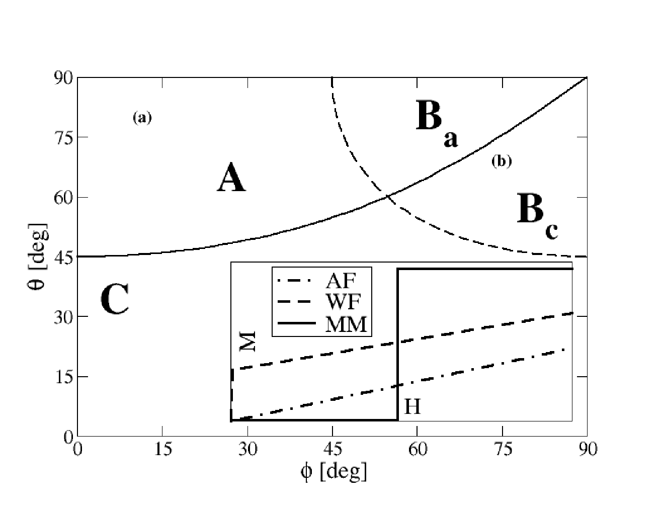
Relaxing the angles and , we have noticed that the sequence of the magnetization patterns varies with the easy axes orientation and we have established the domains (Fig. 2) in the (, ) parameter space. Within a given domain the fixed shape of the low-temperature magnetization isotherms as a function of field for all the crystallographic directions occurs. The expected zero-temperature patterns are plotted in the inset. The sectors appearing in the diagram are described in Table 1. In sectors A, B, C the -type patterns are unveiled for the field along the , , axes, respectively. The sequence of the AF and WF profiles accompanying the -type shape in a given sector is specified in Table 1. In the B sectors the AF pattern is missing and two WF patterns are present in return. The crystallographic direction, where the magnetization values are higher in the low fields, has been distinguished by an additional index (or ).
| Sector | Crystallographic direction | ||
|---|---|---|---|
| symbol | |||
| A | |||
| Ba | |||
| Bc | |||
| C | |||
The B sectors in the diagram are separated from the other sectors by the dashed line obtained from the solution of the equation . This line corresponds to the canted angle between the adjacent anisotropy axes which amounts to . The solid line in the diagram follows from the symmetry of the Hamiltonian and can be determined from the solution of the equation .
The diagram in Fig. 2 provides the criterion whether the model (3) can describe a particular magnetic system. It predicts the occurrence of the -type profile which is accompanied by a given combination of the -type and the -type patterns.
We immediately see that the criterion is fulfilled for Mn-CAF [11]. Its geometric coordinates (, ) belong to the sector C and the experimental single-crystal profiles agree with the patterns predicted for this sector.
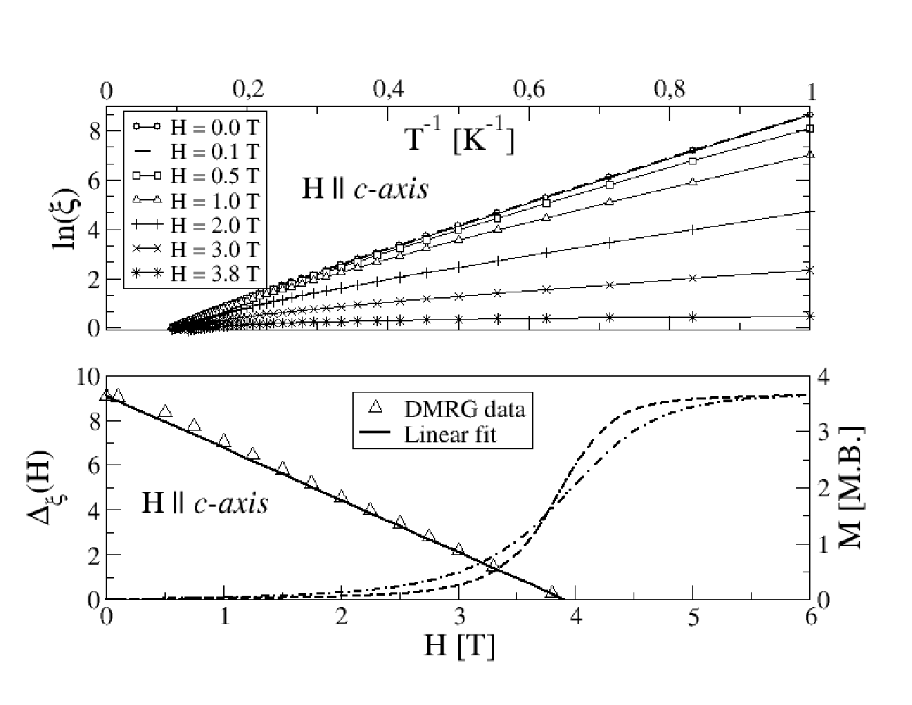
As the zero-field susceptibility and the correlation energy are not related for the canted antiferromagnetic chains, we have decided to analyse the field dependence of the correlation energy . First we checked if the correlation length diverges in the limit of low temperatures. For low temperatures the upper panel of Fig. 3 demonstrates a linear dependence of (where is determined from Eq. (4)) on the inverse of temperature, choosing the Mn-CAF parameters (5) and the corresponding angles and . This dependence implies that the low-temperature correlation length exhibits the exponential divergence in the -direction
| (6) |
but the slope is field dependent.
The field dependence of the correlation energy has been studied numerically and plotted by triangles in the bottom part of Fig (3). We have revealed the striking linear behavior which can be very well reproduced by the function
| (7) |
where the right hand side is expressed in K and the field is given in T. So, the function vanishes, which implies a finite value of correlation length (see Eq. (6)), for the critical field T, what is close to the value estimated directly from the DMRG correlation length, T.
The abrupt change of the correlation length from the infinite to the finite value induced by the field should be accompanied by some changes in the physical properties. We demonstrate in the bottom panel of Fig. 3 that the -type profile displays a rapid jump in the vicinity of T from to a nearly saturation value. We interpret this behavior as a field-driven transition from the antiferromagnetic to the ferromagnetic order along the direction. Such critical field can be determined from the intersection of the low-temperature magnetization isotherms, from their inflection point or from the maximum of the in-field magnetic susceptibility.
Now we analyze the correlation energy for the Mn-CAF parameters in the absence of a magnetic field. The formula (7) implies K, while the DMRG calculations based on Eqs. (1) and (4) yield K. These estimates are in remarkable agreement with the classical prediction [11] K following from Eq. (2). Moreover, the coincidence of the correlation energy of the quantum model (3) and the classical dependence (2) is confirmed and demonstrated for a number of couplings and the canting angles in Fig. 4.
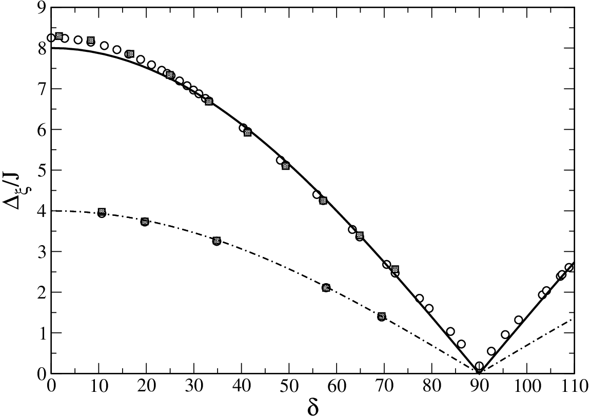
In Fig. 4 the upper continuous and lower dashed lines represent the functions 2S and S, respectively. The open and full circles illustrate the ratios calculated numerically within DMRG for =1.26 K and =1.36 K, respectively. As to the angles , their values follow from the angles and chosen from different sectors of the diagram in Fig. 2. The fields were applied in the proper direction for a sector selected.
We conclude that the agreement between the classical predictions 2S for the ratio and those calculated for our quantum model (3) and plotted in Fig. 4 is very good. There are some deviation for small and high values of , but they can be attributed to uncertainties of the extrapolations performed for ln() yielding the values . These uncertainties are of the order of a few percent and are much higher than the accuracy of the DMRG results. They could be diminished lowering temperature and increasing the cost of our simulations. Concluding, our numerical results in Fig. 4 give a strong evidence that the correlation energy of the canted antiferromagnetic quantum chains can be expressed by the relation (2) previously found for the classical systems.
In Fig. 4 we also plot by the full squares the ratios as a function of , where is the value of the -type magnetization profile corresponding to the field . We emphasise that the ratio is completely determined by the coordinates of the inflection point of the -type magnetization profile. The ratios calculated coincide with the values of the function S drawn by the dashed line and are lower by a factor of 2 than the ratios , implying that
| (8) |
We can interpret the result (8) that the correlation energy is equal to the average Zeeman energy per pair of spins calculated for the critical field .
The relation (8) is an important result of our paper because it provides a direct estimate of the correlation energy in terms of the special coordinates of the -type magnetization profile. Moreover, the exchange constant can be also obtained from the -type single-crystal low-temperature magnetization isotherm. Combining Eqs. (2) and (8), we find the formula for the magnetic coupling
| (9) |
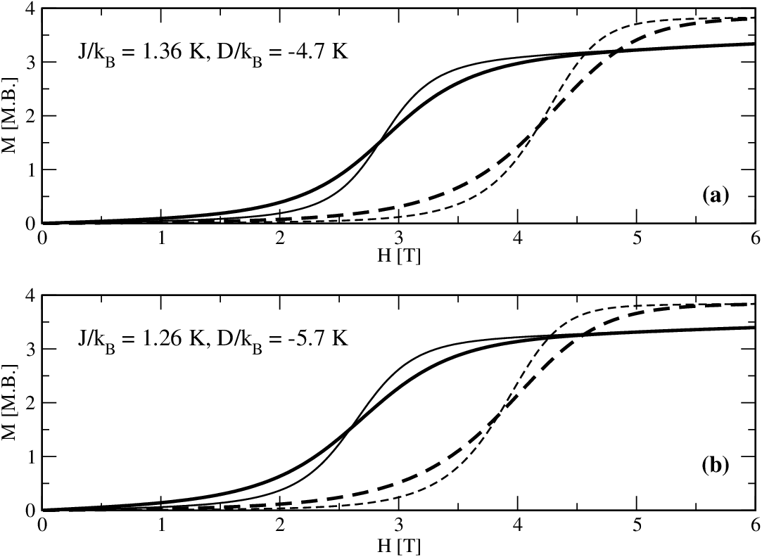
To validate our conclusions, in Fig. 5 the -type behavior is drawn for the ratios and in both panels. For the angles specified in the legends and coming from the sectors A and B, the a and b panels display the profiles found for the magnetic field parallel to the axis and axis, respectively. The slope of all the -type curves in Fig. 5 increases with decreasing temperature and the shape does not change.
The coordinates of the intersections of the corresponding magnetization isotherms in Fig. 5 ( K and K) inserted into Eq. (9) yield the consistent estimates of with the uncertainty equal to K for the input values K and K. When we used lower temperatures ( K and K), the uncertainty declined to K for the same , which is the expected trend.
Now, taking the values deg, T and (in ) directly from the experiment for Mn-CAF compound [11], we can evaluate from Eqs. (8) and (9) the value of correlation energy K and the coupling constant K, respectively. Both the values are slightly lower than the K and K reported earlier [11]. However, this fact can be understood as the experimental value K was settled on the basis of the classical model and the fitting procedure which usually overestimate the coupling constant [20]. If the coupling is overestimated then the relation (2) may proliferate the inaccuracy and imply somewhat higher .
IV Conclusions
Our investigation has confirmed that the relative positions of the anisotropy axes affect the shape of magnetization curves along different crystallographic directions. The resulting angle-dependent diagram predicts four areas, each characterized by a specific sequence of the in-field magnetization patterns. If for a compound studied the shapes of magnetization curves in the low-temperature range are consistent with those established in the diagram for a given geometry, then the compound can be analyzed in terms of the quantum Heisenberg model with a strong anisotropy.
For the canted antiferromagnet SCM the values of correlation energy decrease linearly with the applied field and vanish at which coincides with the intersection point of the -type magnetization profiles. The coordinates and of this special point determine the zero-field correlation energy which in turn reveals the classical dependence on the canting angle and the coupling . These findings relate the value to the coordinates and and yield a simple recipe to the evaluation of .
Following these ideas, we have estimated for the Mn-CAF compound the relevant quantities at K and K which agree very well with the values reported earlier.
Our calculations provide some insight into the common claim that in the strong anisotropy limit the Heisenberg model can be substituted by the Ising model. We confirm that the projections of spins onto the axis displaying the -type pattern can be treated as classical Ising-type variables. Then the rapid jump in the magnetization profile can be related to formation of an Ising domain wall. Anyway, it is striking that the quantity defined in the absence of field can be so easily settled from the experiment performed in the presence of field.
V Acknowledgements
We are grateful to Prof. R. Sessoli for many valuable discussions explaining the structure and properties of the compound considered here. A. B. and G. K. thank to the Polish Ministry of Science and Higher Education for supporting this work under the Iuventus Plus program (IP2010 001170) and Grant Nr 230137, respectively. Numerical calculations were performed in PSNC Poznań (Poland) and WCSS Wrocław (Poland, grant 82). This work was also granted access to the HPC resources within DECI by the PRACE-2IP under grant no RI-283493.
References
- [1] Dante Gatteschi, Roberta Sessoli, and Jacques Villain, Molecular nanomagnets, Oxford University Press, 2006.
- [2] A. Caneschi, D. Gatteschi, N. Lalioti, C. Sangregorio, R. Sessoli, G. Venturi, A. Vindigni, A. Rettori, M. G. Pini, M. A. Novak, Angew. Chem. Int. Ed. 40, 1760 (2001).
- [3] R. Clerac, H. Miyasaka, M. Yamashita, C. Coulon, J. Am. Chem. Soc. 124, 12837 (2002).
- [4] H. Miyasaka, T. Madanbashi, K. Sugimoto, Y. Nakazawa, W. Wernsdorfer, K. Sugiura, M. Yamashita, C. Coulon, R. Clerac, Chem. Eur. J. 12, 7028 (2006).
- [5] C. Coulon, H. Miyasaka, and R. Cleérac, Struct. Bond. 122, 163 (2006); H. Miyasaka and M. Yamashita, Dalton Trans., 399 (2007), and references therein.
- [6] N. B. Ivanov, J. Richter, and U. Schollwoeck, Phys. Rev. B 58, 14456 (2007).
- [7] Y.-Z. Zheng, W. Xue, W.-X. Zhang, M.-L. Tong, X.-M. Chen, F. Grandjean, G. J. Long, S.-W. Ng, P. Panissod, and M. Drillon, Inorg. Chem. 48, 2028 (2009).
- [8] R. J. Glauber, J. Math. Phys. 4, 294 (1963).
- [9] H. Miyasaka, M. Julve, M. Yamashita, and R. Clerac, Inorg. Chem. 48, 3420 (2009).
- [10] M. G. Pini and A. Rettori, Phys. Rev. B 76, 064407 (2007).
- [11] K. Bernot, J. Luzon, R. Sessoli, A. Vindigni, J. Thion, S. Richeter, D. Leclercq, J. Larionova, and A. van der Lee, J. Am. Chem. Soc. 130, 1619 (2008).
- [12] B. Barbara, J. Phys. 34, 1039 (1973).
- [13] J. M. Loveluck, S. W. Lovesey, S. J. Aubry, Phys. C: Solid State Phys. 8, 3841 (1975).
- [14] C. Coulon, R. Clerac, L. Lecren, W. Wernsdorfer, and H. Miyasaka Phys. Rev. B 69, 132408 (2004).
- [15] A. Saitoh, H. Miyasaka, M. Yamashita, and R. Clerac, J. Mater. Chem. 17, 2002 (2007).
- [16] J. Boeckmann, M. Wriedt, C.Näther, Chem. Eur. J. 18, 5284 (2012).
- [17] Y-Z. Zheng, W. Xue, M-L. Tong, X-M. Chen, F. Grandjean, G.J. Long, Inorg. Chem. 47, 4077 (2008)
- [18] Jung Hee Yoon, Dae Won Ryu, Hyoung Chan Kim, Sung Won Yoon, Byoung Jin Suh, and Chang Seop Hong, Chem. Eur. J. 15, 3661 (2009).
- [19] A. Barasiński, G. Kamieniarz, and A. Drzewiński, Comp. Phys. Comm. 182, 2013 (2011).
- [20] P. Sobczak, A. Barasiński, G. Kamieniarz, A. Drzewiński, Phys. Rev. B 84, 224431 (2011).
- [21] G. Kamieniarz, R. Matysiak, A. C. D’Auria, F. Esposito, and U. Esposito, Phys. Rev. B 56, 645 (1997).
- [22] A. Caramico D’Auria, F. Esposito, U. Esposito, D. Gatteschi, G. Kamieniarz, and S. Wałcerz, J. Chem. Phys. 109, 1613 (1998).
- [23] G. Kamieniarz, M. Bieliński, and J.-P. Renard, Phys. Rev. B 60, 14521 (1999).
- [24] R. Matysiak, G. Kamieniarz, P. Gegenwart, and A. Ochiai, Phys. Rev. B 79, 224413 (2009).
- [25] M. Suzuki, Prog. Theor. Phys. 56, 1454 (1976).
- [26] T. Delica and H. Leschke, Physica A 176, 736 (1990).
- [27] X. Q. Wang and T. Xiang, Phys. Rev. B 56, 5061 (1997).
- [28] U. Schollwoeck, Rev. Mod. Phys. 77, 259 (2005); K. Hallberg, Adv. Phys. 55, 477 (2006); U. Schollwoeck, Ann. Phys. (NY) 326, 96 (2011).
- [29] A. Maciołek, A. Drzewiński, and R. Evans, Phys. Rev. B 64, 056137 (2001).
- [30] A. Drzewiński, A. Maciołek, A. Barasiński, and S. Dietrich, Phys. Rev. E 79, 041145 (2009).
- [31] N. Shibata, J. Phys. A: Math. Gen. 36, R381 (2003).
- [32] A. Barasiński, P. Sobczak, A. Drzewiński, G. Kamieniarz, A. Bieńko, J. Mroziński, and D. Gatteschi, Polyhedron 29, 1485 (2010).
- [33] R. J. Baxter, Exactly Solved Models in Statistical Mechanics, Academic Press 1982.
- [34] N. Hatano and M. Suzuki, J. Phys. Soc. J. 62, 1346 (1993).
- [35] G. Kamieniarz, P. Kozlowski, M. Antkowiak, P. Sobczak, T. Ślusarski, D. M. Tomecka, A. Barasiński, B. Brzostowski, A. Drzewiński, A. Bieńko, J. Mroziński, Acta Phys. Pol. A 121, 992 (2012).