Wonder of Sine-Gordon $Y$ -systems

Tomoki Nakanishi Address: Graduate School of Mathematics, Nagoya University, Chikusa-ku, Nagoya, 464-8604, Japan Email address: nakanisi@math.nagoya-u.ac.jp and Salvatore Stella Address: Department of Mathematics, North Carolina State University, Box 8205, Raleigh, NC 27695-8205, USA Email address: sstella@ncsu.edu

Abstract.

The sine-Gordon $Y$ -systems and the reduced sine-Gordon $Y$ -systems were introduced by Tateo in the 90’s in the study of the integrable deformation of conformal field theory by the thermodynamic Bethe ansatz method. The periodicity property and the dilogarithm identities concerning these $Y$ -systems were conjectured by Tateo, and only a part of them have been proved so far. In this paper we formulate these $Y$ -systems by the polygon realization of cluster algebras of types $A$ and $D$ , and prove the conjectured periodicity and dilogarithm identities in full generality. As it turns out, there is a wonderful interplay among continued fractions, triangulations of polygons, cluster algebras, and $Y$ -systems.

2010 Mathematics Subject Classification

13F60, 17B37

Refer to caption — Figure 1. Initial triangulation of 106-gon for SG $Y$ -system $\mathbb{Y}_{\mathrm{SG}}(6,4,3)$ .

1. Introduction

In the 90’s the integrable deformation of conformal field theory was intensively studied by the thermodynamic Bethe ansatz method. As a consequence, several periodicities of the so-called $Y$ -systems and the associated dilogarithm identities were conjectured. However, at that time there was no systematic mathematical framework to prove these conjectures. As a result, most of them were left open. Since the pioneering work by Fomin and Zelevinsky [FZ02, FZ03b], it has been gradually noticed that these periodicities of $Y$ -systems in fact come from periodicities of cluster algebras. In this way the periodicities and dilogarithm identities conjectured for the major family of $Y$ -systems originated from quantum affine algebras were proved using the cluster algebraic formulation [Cha05, Kel10, Kel13, Nak11a, IIK+13a, IIK+13b]. Simultaneously, an efficient method of proving periodicities in cluster algebras has been also developed by combining tropicalization and categorification technique [IIK+13a, Pla11].

Another interesting family of $Y$ -systems was introduced by Tateo [Tat95a] in the same context. It consists of two subfamilies called the sine-Gordon (SG) $Y$ -systems and the reduced sine-Gordon (RSG) $Y$ -systems, respectively. They are exotic in several senses. Firstly, the Lie theoretic interpretation is not entirely clear, though they are certainly related to the Virasoro algebra, $U_{q}(\widehat{sl}_{2})$ at a root of unity, etc. Secondly, they are associated with continued fractions. Thirdly, they are systems of functional equations, some of which appear to be very complicated. In the same paper Tateo also conjectured the periodicity and the dilogarithm identities for these $Y$ -systems. Soon later, Gliozzi and Tateo [GT96] ingeniously found a general solution for the RSG $Y$ -systems in terms of cross-ratios, and thereby proved their periodicity. However, other conjectures were left open. The reason for the existence of such a simple solution for a very complicated system also remained a mystery.

Recently, Tateo and the first author [NT10] formulated a (small) part of the SG/RSG $Y$ -systems by cluster algebras, then proved their periodicity and the associated dilogarithm identities by applying the aforementioned tropicalization-categorification method. However, due to the complexity of these $Y$ -systems, working out the conjecture in full generality by this method seemed not easy.

In this paper we prove Tateo’s conjectures on periodicity and dilogarithm identities of the SG/RSG $Y$ -systems in full generality. The basic strategy to overcome the above difficulty is the following. As the referee of the paper [NT10] pointed out, the cluster algebras for the RSG and SG $Y$ -systems therein are nothing but cluster algebras of types $A$ and $D$ , respectively. Suppose that it is true in general. It is well known that the cluster algebras of types $A$ and $D$ admit a surface realization developed by [GSV05, FZ03a, FG07, FST08, FT12]. To be more specific, they are realized by polygons without puncture for type $A$ and with one puncture for type $D$ . So, we may try to realize these $Y$ -systems by polygons. It turns out that this is possible; moreover, the nature of these $Y$ -systems becomes most apparent in the polygon realization.

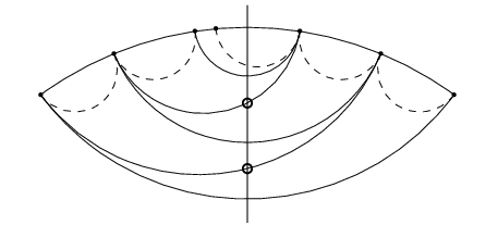
Let us briefly explain how our method works. For a given SG/RSG $Y$ -system, the construction of the initial triangulation of a polygon is our first step, and it is strongly tied with the theory of continued fractions, as we should expect. In fact, this triangulation is directly associated with the continued fraction which parametrizes the SG/RSG $Y$ -system. The next key observation is that the above triangulation has a remarkable quasi-symmetry with respect to two axes of the polygon; moreover, the mutations realizing the $Y$ -system are simply the reflections with respect to these axes. For example, Figure 1 represents the initial triangulation (a tagged triangulation in the sense of [FST08]) of a 106-gon with a puncture corresponding to the SG $Y$ -system associated with the continued fraction

(1.1)

\displaystyle[3,4,6]:=\frac{1}{\displaystyle 3+\frac{1}{\displaystyle 4+\frac{1}{6}}}=\frac{25}{81}.

The number 106 comes from $25+81=106$ . Observe that the triangulation is almost symmetric with respect to the two axes therein; moreover, flipping (mutating) the diagonals which cross one of the axes and are not symmetric with respect to it, we get the reflection. Composing these two reflections, we get a rotation. This geometric realization of the SG/RSG $Y$ -system enables us to prove the conjectured periodicities at once; they are nothing but the full rotations of the associated polygons. From these triangulations, we can also reconstruct the cross-ratio solution of the RSG $Y$ -systems by [GT96] naturally. Furthermore, the conjectured dilogarithm identities reduce to a simple geometrical counting problem for the triangulations.

Throughout our work we found a wonderful interplay among continued fractions, triangulations of polygons, cluster algebras, and $Y$ -systems. This is perhaps the most important message of the paper. Also, we ask the reader not to be discouraged by the “horrible appearance” of the RSG/SG $Y$ -systems in Section 3, since they are beautiful in nature, as you see in Figure 1.

The paper is organized as follows. In Section 2 we recall some basic properties of continued fractions. In Section 3 we introduce the RSG/SG $Y$ -systems. In Section 4, using some examples, we explain in detail how to realize the RSG $Y$ -systems by polygons. In particular, we introduce the snapshot method to obtain the relations in these $Y$ -systems. Section 5 is the main part of the paper. To any continued fraction we construct the associated triangulation of a polygon, and we show that it provides a realization of the corresponding RSG $Y$ -system. As a result, we obtain the periodicity of the RSG $Y$ -systems, and also reproduce the solution by Gliozzi-Tateo. In Section 6 we adapt our construction of the triangulation for a polygon with a puncture. Then, we show that it provides a realization of the corresponding SG $Y$ -system. As a result, we obtain the periodicity of the SG $Y$ -systems. In Section 7 we prove the dilogarithm identities conjectured by Tateo. In Section 8 we introduce the RSG/SG $T$ -systems accompanying the RSG/SG $Y$ -systems. They share the same periodicity with the RSG/SG $Y$ -systems.

Acknowledgements. We thank Hugh Thomas and Dylan Thurston for useful discussion. We thank MSRI, Berkeley for financial support and for providing the ideal environment where this work was done. The second author is partially supported by A. Zelevinsky’s NSF grant DMS-1103813.

2. Continued fractions

Before starting, let us summarize some useful properties of continued fractions which will be used throughout the paper. The results are standard in the literature (e.g., [Wal48]).

First, we fix an arbitrarily positive integer $F$ . Then, we fix a sequence of positive integers $(n_{1},\dots,n_{F})$ with $n_{1}\geq 2$ . This is our input data. The sequence $(n_{1},\dots,n_{F})$ determines a rational number $0<\xi<1$ by the continued fraction

(2.1)

\displaystyle\xi

\displaystyle=[n_{F},\dots,n_{1}]:=\frac{1}{\displaystyle n_{F}+\frac{1}{\displaystyle n_{F-1}+\frac{1}{{\displaystyle\ddots+\frac{1}{\displaystyle n_{1}}}}}}.

To make it clear, $[n_{1}]=1/n_{1}$ . Conversely, any rational number $0<\xi<1$ is uniquely expressed in this form. Therefore, the correspondence is one-to-one. The order of the subscript of $n_{i}$ is opposite to the standard one, but this is convenient for our purpose.

For the sequence $(n_{1},\dots,n_{F})$ , we introduce a family of continued fractions

(2.2)

\displaystyle\xi_{a}

\displaystyle=[n_{a},\dots,n_{1}],\quad 1\leq a\leq F.

We write $\xi_{a}$ with coprime integers $p_{a}$ , $q_{a}$ as

(2.3)

\displaystyle\xi_{a}=\frac{p_{a}}{q_{a}},\quad 1\leq a\leq F.

In particular, $(p_{1},q_{1})=(1,n_{1})$ . Since $\xi_{a}=1/(n_{a}+\xi_{a-1})$ for $2\leq a\leq F$ , we have

(2.4)

\displaystyle\frac{p_{a}}{q_{a}}=\frac{1}{n_{a}+\displaystyle\frac{p_{a-1}}{q_{a-1}}}=\frac{q_{a-1}}{n_{a}q_{a-1}+p_{a-1}}.

Then, thanks to the coprime property, we have the relations

(2.5)		$\displaystyle p_{a}$	$\displaystyle=q_{a-1},\quad 2\leq a\leq F,$
(2.6)		$\displaystyle q_{a}$	$\displaystyle={n_{a}q_{a-1}+p_{a-1}},\quad 2\leq a\leq F.$

Thus, all $p_{a}$ and $q_{a}$ are determined from the recursion relations,

(2.7)		$\displaystyle q_{a}$	$\displaystyle=n_{a}q_{a-1}+q_{a-2},\quad 2\leq a\leq F,$
(2.8)		$\displaystyle p_{a}$	$\displaystyle=n_{a-1}p_{a-1}+p_{a-2},\quad 3\leq a\leq F,$

with the initial condition $q_{0}:=1$ , $q_{1}=n_{1}$ , $p_{1}=1$ , $p_{2}=n_{1}$ .

More generally, for the same sequence $(n_{1}$ , …, $n_{F})$ and for any $k=1,\dots,F$ , we introduce a family of continued fractions

(2.9)

\displaystyle\xi^{(k)}_{a}=[n_{a},\dots,n_{k}],\quad k\leq a\leq F.

Thus, $\xi_{a}=\xi^{(1)}_{a}$ , though we mainly use the former notation, since they are the “principals”. We write $\xi^{(k)}_{a}$ with coprime integers $p^{(k)}_{a}$ , $q^{(k)}_{a}$ as

(2.10)

\displaystyle\xi^{(k)}_{a}=\frac{p^{(k)}_{a}}{q^{(k)}_{a}},\quad k\leq a\leq F.

In particular, $(p^{(k)}_{k},q^{(k)}_{k})=(1,n_{k})$ . Then, by the same argument as before, we have $p^{(k)}_{a}=q^{(k)}_{a-1}$ , and all $p^{(k)}_{a}$ and $q^{(k)}_{a}$ are determined from the recursion relations,

(2.11)		$\displaystyle q^{(k)}_{a}$	$\displaystyle=n_{a}q^{(k)}_{a-1}+q^{(k)}_{a-2},\quad k+1\leq a\leq F,$
(2.12)		$\displaystyle p^{(k)}_{a}$	$\displaystyle=n_{a-1}p^{(k)}_{a-1}+p^{(k)}_{a-2},\quad k+2\leq a\leq F,$

with the initial condition $q^{(k)}_{k-1}:=1$ , $q^{(k)}_{k}=n_{k}$ , $p^{(k)}_{k}=1$ , $p^{(k)}_{k+1}=n_{k}$ . We define integers

(2.13)

\displaystyle r^{(k)}:=p^{(k)}_{F}+q^{(k)}_{F},\quad 1\leq k\leq F,

and we especially write $r^{(1)}$ as $r$ in accordance with the notation $\xi_{F}=\xi^{(1)}_{F}$ .

Example 2.1.

We use the following data as a running example throughout the paper: For $F=3$ , $(n_{1},n_{2},n_{3})=(6,4,3)$ , we have

(2.14)	$\displaystyle\xi_{1}$	$\displaystyle=\frac{1}{6},$	$\displaystyle\quad(p_{1},q_{1})$	$\displaystyle=(1,6),$
(2.15)	$\displaystyle\xi_{2}$	$\displaystyle=\frac{1}{4+\frac{1}{6}}=\frac{6}{25},$	$\displaystyle\quad(p_{2},q_{2})$	$\displaystyle=(6,25),$
(2.16)	$\displaystyle\xi_{3}$	$\displaystyle=\frac{1}{3+\frac{6}{25}}=\frac{25}{81},$	$\displaystyle\quad(p_{3},q_{3})$	$\displaystyle=(25,81),$	$\displaystyle\quad r$	$\displaystyle=106,$
(2.17)	$\displaystyle\xi^{(2)}_{2}$	$\displaystyle=\frac{1}{4},$	$\displaystyle\quad(p^{(2)}_{2},q^{(2)}_{2})$	$\displaystyle=(1,4),$
(2.18)	$\displaystyle\xi^{(2)}_{3}$	$\displaystyle=\frac{1}{3+\frac{1}{4}}=\frac{4}{13},$	$\displaystyle\quad(p^{(2)}_{3},q^{(2)}_{3})$	$\displaystyle=(4,13),$	$\displaystyle\quad r^{(2)}$	$\displaystyle=17,$
(2.19)	$\displaystyle\xi^{(3)}_{3}$	$\displaystyle=\frac{1}{3},$	$\displaystyle\quad(p^{(3)}_{3},q^{(3)}_{3})$	$\displaystyle=(1,3),$	$\displaystyle\quad r^{(3)}$	$\displaystyle=4.$

The following formulas are well known (e.g., [Wal48]).

Proposition 2.2.

(a). (Fundamental recurrence formulas) For $k=1,\dots,F-2$ , we have

(2.20)		$\displaystyle q^{(k)}_{a}$	$\displaystyle=n_{k}q^{(k+1)}_{a}+q^{(k+2)}_{a},\quad k+2\leq a\leq F,$
(2.21)		$\displaystyle p^{(k)}_{a}$	$\displaystyle=n_{k}p^{(k+1)}_{a}+p^{(k+2)}_{a},\quad k+2\leq a\leq F.$

(b). For $k=1,\dots,F-1$ , we have

(2.22)

\displaystyle q^{(k)}_{a}p^{(k+1)}_{a}-q^{(k+1)}_{a}p^{(k)}_{a}=(-1)^{a-k+1},\quad k+1\leq a\leq F.

Proof.

(a). They are easily proved by induction on $a$ using (2.12). (b). For each $a$ , this is proved by induction on $k$ in the decreasing order using (a). ∎

We will also use the following properties later.

Proposition 2.3.

(a). For $k=1,\dots,F$ , we have

(2.23)

\displaystyle r^{(k)}

\displaystyle=n_{k}r^{(k+1)}+r^{(k+2)},

where we set $r^{(F+1)}=r^{(F+2)}:=1$ .

(b). For $k=1,\dots,F$ , we have

(2.24)

\displaystyle r^{(k)}

\displaystyle=q^{(k)}_{a}r^{(a+1)}+p^{(k)}_{a}r^{(a+2)},\quad k\leq a\leq F.

For $a=k$ , it reduces to (a).

(c). For each $a=2,\dots,F$ , the numbers $p_{a}$ and $p^{(2)}_{a}$ are coprime.

(d). The numbers $r$ and $r^{(2)}$ are coprime.

(e). For $a=3,\dots,F$ , we have

(2.25)

\displaystyle p_{a-1}p^{(2)}_{a}-p_{a}p^{(2)}_{a-1}=(-1)^{a}.

Proof.

(a). For $k\leq F-2$ , this is a corollary of Proposition 2.2 (a). For $k=F-1,F$ , this is checked by direct inspection; indeed $r^{(F-1)}=n_{F-1}(n_{F}+1)+1$ and $r^{(F)}=n_{F}+1$ . (b). This can be proved by induction on $a$ using (2.12) and (2.23). (c). Using (2.21) repeatedly, we have $\mathrm{gcd}(p_{a},p^{(2)}_{a})=\mathrm{gcd}(p^{(3)}_{a},p^{(2)}_{a})=\cdots=\mathrm{gcd}(p^{(a-1)}_{a},p^{(a)}_{a})=1.$ The claim also follows from (e) below. (d). Using (2.23) repeatedly, we have $\mathrm{gcd}(r^{(k)},r^{(k+1)})=\mathrm{gcd}(r^{(k+2)},r^{(k+1)})=\cdots=\mathrm{gcd}(r^{(F)},r^{(F+1)})=1.$ (e). This is a special case of Proposition 2.2 (b) with $k=1$ . ∎

3. RSG and SG $Y$ -systems

Here we introduce the RSG and SG $Y$ -systems following [Tat95a]. For the background of these equations in conformal field theory, consult [Tat95b, Tat95a] and [NT10, Section 2.3]. Then we state the periodicity property of these $Y$ -systems.

3.1. RSG $Y$ -systems

We continue to use the sequence $(n_{1},\dots,n_{F})$ in the previous section as input data. We exclude the case $(n_{1})=(2)$ with $F=1$ , because the RSG $Y$ -system is empty.

We introduce the notation for the signs

(3.1)

\displaystyle\varepsilon_{a}:=(-1)^{a-1},\quad a=1,\dots,F.

We start with the case $n_{1}\neq 2$ . Let us introduce the $Y$ -variables $Y^{(a)}_{m}(u)$ , where $u\in\mathbb{Z}$ , $a=1\dots,F$ , and

(3.2)

\displaystyle m=\begin{cases}1,\dots,n_{1}-2&\mbox{if $a=1$}\\ 1,\dots,n_{a}&\mbox{if $a=2,\dots,F$}.\end{cases}

Let $X_{\mathrm{RSG}}(n_{1},\dots,n_{F})$ be the Dynkin diagram of type $A$ indexed by $(a,m)$ in the above range as shown in Figure 2.

Figure 2. The diagram

X_{\mathrm{RSG}}(n_{1},\dots,n_{F})

for

n_{1}\neq 2

Definition 3.1.

For $n_{1}\neq 2$ , the reduced sine-Gordon (RSG) $Y$ -system $\mathbb{Y}_{\mathrm{RSG}}(n_{1},\dots,n_{F})$ is the following system of relations: For a general $(a,m)$ other than $(2,1)$ , $(3,1)$ , …, $(F,1)$ ,

(3.3)

\displaystyle Y^{(a)}_{m}(u-p_{a})Y^{(a)}_{m}(u+p_{a})

\displaystyle=\prod_{(b,k)\sim(a,m)}(1+Y^{(b)}_{k}(u)^{\varepsilon_{b}})^{\varepsilon_{b}},

where $(b,k)\sim(a,m)$ means $(b,k)$ is adjacent to $(a,m)$ in the diagram $X_{\mathrm{RSG}}(n_{1},\dots,n_{F})$ , and $p_{a}$ ( $1\leq a\leq F$ ) are the numbers defined in (2.3). Exceptional cases are as follows. For $(a,m)=(2,1)$ ,

(3.4)

\displaystyle\begin{split}&Y^{(2)}_{1}(u-p_{2})Y^{(2)}_{1}(u+p_{2})\\ &\qquad=(1+Y^{(2)}_{2}(u)^{-1})^{-1}(1+Y^{(1)}_{1}(u))\\ &\qquad\quad\times\prod_{m=1}^{n_{1}-2}(1+Y^{(1)}_{m}(u-1-m)^{-{1}})^{-{1}}(1+Y^{(1)}_{m}(u+1+m)^{-{1}})^{-{1}}.\end{split}

For $(a,m)=(a,1)$ with $a=3,\dots,F$ ,

(3.5)

\displaystyle\begin{split}&Y^{(a)}_{1}(u-p_{a})Y^{(a)}_{1}(u+p_{a})\\ &\qquad=(1+Y^{(a)}_{2}(u)^{\varepsilon_{a}})^{\varepsilon_{a}}(1+Y^{(a-2)}_{n_{a-2}-2\delta_{a3}}(u)^{\varepsilon_{a}})^{\varepsilon_{a}}\\ &\qquad\quad\times\prod_{m=1}^{n_{a-1}}(1+Y^{(a-1)}_{m}(u-p_{a}+(n_{a-1}+1-m)p_{a-1})^{\varepsilon_{a}})^{\varepsilon_{a}}\\ &\qquad\quad\times\prod_{m=1}^{n_{a-1}}(1+Y^{(a-1)}_{m}(u+p_{a}-(n_{a-1}+1-m)p_{a-1})^{\varepsilon_{a}})^{\varepsilon_{a}},\end{split}

where $\delta_{a3}$ is the Kronecker delta.

Remark 3.2.

The variables $Y_{1}(u)$ , $Y_{2}(u)$ , …in [Tat95a] and [NT10] are $Y^{(F)}_{n_{F}}(u)$ , $Y^{(F)}_{n_{F}-1}(u)$ , …, $Y^{(F-1)}_{n_{F-1}}(u)$ , …, $Y^{(1)}_{1}(u)$ here with a certain rescale of $u$ , and also up to the opposite convention of the sign $\varepsilon_{a}$ for even $F$ .

When $F=1$ , only the relation (3.3) is involved. This is the well known $Y$ -system of type $A_{n_{1}-2}$ (with level 2, in the terminology of [KNS94]). So, the RSG $Y$ -systems are generalizations of the $Y$ -systems of type $A$ .

When $n_{1}=2$ with $F\geq 2$ , we need some modification. We reset the $Y$ -variables $Y^{(a)}_{m}(u)$ , where $u\in\mathbb{Z}$ , $a=2\dots,F$ , and $m=1,\dots,n_{a}$ . Let $X_{\mathrm{RSG}}(2,n_{2},\dots,n_{F})$ be the tadpole diagram indexed by $(a,m)$ in the above range as shown in Figure 3.

Definition 3.3.

For $F\geq 2$ , the RSG $Y$ -system $\mathbb{Y}_{\mathrm{RSG}}(2,n_{2},\dots,n_{F})$ is the following system of relations:

(i).

the relation (3.3) for $(a,m)$ other than $(3,1),\dots,(F,1)$ , where the adjacency diagram for (3.3) is $X_{\mathrm{RSG}}(2,n_{2},\dots,n_{F})$ ,
(ii).

the relation (3.5) for $(a,1)$ with $a=3,\dots,F$ , where for $a=3$ the term $Y^{(1)}_{0}(u)$ in the right hand side of (3.5) is discarded.

Figure 3. The diagram

X_{\mathrm{RSG}}(2,n_{2},\dots,n_{F})

When $F=2$ , only the relation (3.3) is involved. This is the well known $Y$ -system of tadpole type $T_{n_{2}}$ of [RTV93]). So, these RSG $Y$ -systems are generalizations of the $Y$ -systems of tadpole type.

All main results in the paper are applicable, whether $n_{1}\neq 2$ or $n_{1}=2$ . To make the description simpler, from now on we do not pay a special attention to the exceptional case $n_{1}=2$ when claiming and proving general statements. The reader can safely concentrate on the case $n_{1}\neq 2$ .

Now let us return to Definition 3.1. In the right hand side of (3.4), we have

(3.6)

\displaystyle u-p_{2}+1\leq u-1-m\leq u-2

thanks to $p_{2}=n_{1}$ and $p_{1}=1$ . Also, in the right hand side of (3.5), we have

(3.7)

\displaystyle u-p_{a}+p_{a-1}\leq u-p_{a}+(n_{a-1}+1-m)p_{a-1}\leq u-p_{a-2}

thanks to the relation $-p_{a}+n_{a-1}p_{a-1}=-p_{a-2}$ in (2.8).

Let $\mathcal{Y}=\mathcal{Y}_{\mathrm{RSG}}(n_{1},\dots,n_{F})$ be the set of all $Y$ -variables of $\mathbb{Y}_{\mathrm{RSG}}(n_{1},\dots,n_{F})$ . Let $\mathcal{Y}_{+}$ (resp. $\mathcal{Y}_{-}$ ) be the subset of $\mathcal{Y}$ consisting of $Y^{(a)}_{m}(u)$ such that the integer

(3.8)

\displaystyle\theta^{(a)}_{m}(u):=u+p_{a+1}-(n_{a}-m)p_{a}

is even (resp. odd). It is easy to check the following property.

Proposition 3.4.

In each relation of the $Y$ -system $\mathbb{Y}_{\mathrm{RSG}}(n_{1},\dots,n_{F})$ , if the variables in the left hand side are in $\mathcal{Y}_{+}$ (resp. $\mathcal{Y}_{-}$ ), then the variables in the right hand side are also in $\mathcal{Y}_{+}$ (resp. $\mathcal{Y}_{-}$ ).

Therefore, one can bisect the RSG $Y$ -system into the one for $\mathcal{Y}_{+}$ and the one for $\mathcal{Y}_{-}$ . They are equivalent systems related by the shift of the parameter $u\rightarrow u+1$ . So it is enough to concentrate on the $Y$ -systems for $\mathcal{Y}_{+}$ .

3.2. SG $Y$ -systems

Again, we exclude the case $(n_{1})=(2)$ with $F=1$ , because the SG $Y$ -system is equivalent to the RSG $Y$ -system with $(n_{1})=(5)$ with $F=1$ .

Let us reset the $Y$ -variables $Y^{(a)}_{m}(u)$ , where $u\in\mathbb{Z}$ , $a=1\dots,F$ , and

(3.9)

\displaystyle m=\begin{cases}\overline{1},\overline{2},0,1,\dots,n_{1}-2&\mbox{if $a=1$}\\ 1,\dots,n_{a}&\mbox{if $a=2,\dots,F$}.\end{cases}

Note that the three indices $\overline{1}$ , $\overline{2}$ , $0$ are added for $a=1$ . Let $X_{\mathrm{SG}}(n_{1},\dots,n_{F})$ be the Dynkin diagram of type $D$ indexed by $(a,m)$ in the above range as shown in Figure 4.

Figure 4. The diagram

X_{\mathrm{SG}}(n_{1},\dots,n_{F})

Definition 3.5.

The sine-Gordon (SG) $Y$ -system $\mathbb{Y}_{\mathrm{SG}}(n_{1},\dots,n_{F})$ is the following system of relations:

(i).

the relation (3.3) for $(a,m)$ other than $(2,1)$ , $(3,1)$ , …, $(F,1)$ , where the adjacency diagram for (3.3) is replaced with $X_{\mathrm{SG}}(n_{1},\dots,n_{F})$ ,

(ii).

the relation for $(a,m)=(2,1)$ ,

(3.10)

\displaystyle\begin{split}&Y^{(2)}_{1}(u-p_{2})Y^{(2)}_{1}(u+p_{2})\\ &\qquad=(1+Y^{(2)}_{2}(u)^{-1})^{-1}(1+Y^{(1)}_{\overline{1}}(u)^{-1})^{-1}(1+Y^{(1)}_{\overline{2}}(u)^{-1})^{-1}\\ &\qquad\quad\times\prod_{m=0}^{n_{1}-2}(1+Y^{(1)}_{m}(u-1-m)^{-{1}})^{-{1}}(1+Y^{(1)}_{m}(u+1+m)^{-{1}})^{-{1}},\end{split}

(iii).

the relation (3.5) for $(a,m)=(a,1)$ with $a=3,\dots,F$ .

When $F=1$ , only the relation (3.3) is involved. This is the well known $Y$ -system of type $D_{n_{1}+1}$ (with level 2). So, the SG $Y$ -systems are generalizations of the $Y$ -systems of type $D$ .

As the name suggests, the RSG $Y$ -system $\mathbb{Y}_{\mathrm{RSG}}(n_{1},\dots,n_{F})$ is obtained from $\mathbb{Y}_{\mathrm{SG}}(n_{1},\dots,n_{F})$ by the following reduction [Tat95a]. The relation (3.3) at $(a,m)=(1,0)$ reads

(3.11)

\displaystyle Y^{(1)}_{0}(u-1)Y^{(1)}_{0}(u+1)=(1+Y^{(1)}_{1}(u))(1+Y^{(1)}_{\overline{1}}(u))(1+Y^{(1)}_{\overline{2}}(u)).

Thus, (3.10) is equivalent to

(3.12)

\displaystyle\begin{split}&Y^{(2)}_{1}(u-p_{2})Y^{(2)}_{1}(u+p_{2})\\ &\qquad=Y^{(1)}_{\overline{1}}(u)Y^{(1)}_{\overline{2}}(u)(1+Y^{(2)}_{2}(u)^{-1})^{-1}(1+Y^{(1)}_{1}(u))\\ &\qquad\quad\times(1+Y^{(1)}_{0}(u-1))^{-{1}}(1+Y^{(1)}_{0}(u+1))^{-{1}}\\ &\qquad\quad\times\prod_{m=1}^{n_{1}-2}(1+Y^{(1)}_{m}(u-1-m)^{-{1}})^{-{1}}(1+Y^{(1)}_{m}(u+1+m)^{-{1}})^{-{1}}.\end{split}

Then, under the specialization

(3.13)

\displaystyle Y^{(1)}_{0}(u)=0,\quad Y^{(1)}_{\overline{1}}(u)=Y^{(1)}_{\overline{2}}(u)=-1,

$\mathbb{Y}_{\mathrm{SG}}(n_{1},\dots,n_{F})$ reduces to $\mathbb{Y}_{\mathrm{RSG}}(n_{1},\dots,n_{F})$ .

Let $\mathcal{Y}=\mathcal{Y}_{\mathrm{SG}}(n_{1},\dots,n_{F})$ be the set of all $Y$ -variables of $\mathbb{Y}_{\mathrm{SG}}(n_{1},\dots,n_{F})$ . Let $\mathcal{Y}_{+}$ (resp. $\mathcal{Y}_{-}$ ) be the subset of $\mathcal{Y}$ consisting of $Y^{(a)}_{m}(u)$ such that the integer

(3.14)

\displaystyle\theta^{(a)}_{m}(u):=\begin{cases}u+p_{a+1}-(n_{a}-m)p_{a}&(a,m)\neq(1,\overline{1}),(1,\overline{2})\\ u+1&(a,m)=(1,\overline{1}),(1,\overline{2})\\ \end{cases}

is even (resp. odd).

Again, it is easy to check the following property.

Proposition 3.6.

In each relation of the $Y$ -system $\mathbb{Y}_{\mathrm{SG}}(n_{1},\dots,n_{F})$ , if the variables in the left hand side are in $\mathcal{Y}_{+}$ (resp. $\mathcal{Y}_{-}$ ), then the variables in the right hand side are also in $\mathcal{Y}_{+}$ (resp. $\mathcal{Y}_{-}$ ).

So, it is enough to concentrate on the SG $Y$ -systems for $\mathcal{Y}_{+}$ .

3.3. Periodicity

The first main result of the paper is to prove the following remarkable periodicity of the RSG and SG $Y$ -systems conjectured by [Tat95a].

Recall that $r=r^{(1)}$ is the number defined in (2.13).

Theorem 3.7 ([GT96]).

The RSG $Y$ -system $\mathbb{Y}_{\mathrm{RSG}}(n_{1},\dots,n_{F})$ has the following periodicity.

(3.15)

\displaystyle Y^{(a)}_{m}(u+2r)=Y^{(a)}_{m}(u).

Furthermore, the above period is the minimal one except for the trivial case $(n_{1})=(3)$ with $F=1$ , where, not $2r$ , but $r=4$ is the minimal one.

Theorem 3.8 ([NT10] for $F=2$ ).

The SG $Y$ -system $\mathbb{Y}_{\mathrm{SG}}(n_{1},\dots,n_{F})$ has the following periodicity.

(i). If $r$ is even, we have

(3.16)

\displaystyle Y^{(a)}_{m}(u+2r)=Y^{(a)}_{m}(u).

(ii). If $r$ is odd, we have

(3.17)		$\displaystyle\mbox{(half periodicity)}\quad Y^{(a)}_{m}(u+2r)$	$\displaystyle=\begin{cases}Y^{(1)}_{\overline{2}}(u)&(a,m)=(1,\overline{1})\\ Y^{(1)}_{\overline{1}}(u)&(a,m)=(1,\overline{2})\\ Y^{(a)}_{m}(u)&\mbox{otherwise},\end{cases}$
(3.18)		$\displaystyle\mbox{(full periodicity)}\quad Y^{(a)}_{m}(u+4r)$	$\displaystyle=Y^{(a)}_{m}(u).$

Furthermore, the above period is the minimal one.

Theorem 3.7 was proved in [GT96] by solving the $Y$ -system in terms of cross-ratios of $r$ points. Also, Theorems 3.7 and 3.8 were proved by [NT10] for $F=2$ by the cluster algebraic formulation of the RSG and SG $Y$ -systems.

Proofs of Theorems 3.7 and 3.8 will be given in Sections 5.6 and 6.2, respectively.

Remark 3.9.

(a). The statement of periodicity in Theorem 3.8 was not correctly stated in [Tat95a] in the case $r$ is even, and corrected in the above form in [NT10] in the case of $F=2$ . (For $F=1$ , it is well known [FZ07].)

(b). The following (half) periodicity property of the RSG $Y$ -systems for $F=1$ is well known [GT96, FS95]): For $\mathbb{Y}_{\mathrm{RSG}}(n_{1})$ ,

(3.19)

\displaystyle Y^{(1)}_{m}(u+r)=Y^{(1)}_{n_{1}-1-m}(u).

For $n_{1}=3$ , it degenerates to the full periodicity, so that we have the exception in Theorem 3.7.

(c). Theorem 3.7 also follows from Theorem 3.8 by the reduction (3.13).

4. Example: RSG $Y$ -system $\mathbb{Y}_{\mathrm{RSG}}(6,4,3)$

We start from the formulation of the RSG $Y$ -systems by polygons. It is simpler than the one for the SG $Y$ -systems, because we do not have to consider punctures.

In this section we concentrate on our running example $F=3$ , $(n_{1},n_{2},n_{3})=(6,4,3)$ set in Example 2.1. We explain in detail how to formulate the RSG $Y$ -system $\mathbb{Y}_{\mathrm{RSG}}(6,4,3)$ by a $106$ -gon, where $106=r$ for $(6,4,3)$ , and also how to prove the periodicity. We heuristically derive the construction of its polygon realization in three steps along the generations. Once we understand the essence of this example, the generalization is not so difficult.

4.1. Mutation in cluster algebras

Here we recall (a part of) the mutation rule of a cluster algebra with coefficients. See [FZ07] for detail. Let $(B,y)$ be a labeled $Y$ -seed, consisting of an exchange matrix $B=(b_{ij})_{i,j\in I}$ , and a coefficient tuple $y=(y_{i})_{i\in I}$ , where coefficients $y_{i}$ are in the universal semifield generated by the initial coefficients. The mutation $(B^{\prime},y^{\prime})=\mu_{k}(B,y)$ at $k\in I$ is defined by the following rule.

(4.1)		$\displaystyle b^{\prime}_{ij}$	$\displaystyle=\begin{cases}-b_{ij}&\mbox{$i=k$ or $j=k$}\\ b_{ij}+b_{ik}[b_{kj}]_{+}+[-b_{ik}]_{+}b_{kj}&i,j\neq k,\end{cases}$
(4.2)		$\displaystyle y^{\prime}_{i}$	$\displaystyle=\begin{cases}y_{i}^{-1}&i=k\\ \displaystyle y_{i}\frac{(1+y_{k})^{[-b_{ki}]_{+}}}{(1+y_{k}^{-1})^{[b_{ki}]_{+}}}&i\neq k,\end{cases}$

where $[a]_{+}=a$ for $a>0$ and $0$ otherwise. The relation (4.2) is called the exchange relation for coefficients ( $y$ -variables).

Following the convention of [FST08, FT12], we identify a triangulation of a polygon with a skew-symmetric matrix $B$ in the following way: each diagonal is identified with a label $i$ of $B$ , and if two diagonals $i$ and $j$ share a common triangle, and $j$ follows $i$ anticlockwise (resp. clockwise), then $b_{ij}=1$ (resp. $b_{ij}=-1$ ). Otherwise, $b_{ij}=0$ . For example, for the following triangle

(4.3)

we have $b_{ki}=1$ and $b_{kj}=-1$ .

By the mutation at $k$ , the diagonal $k$ flips as follows.

(4.4)

Meanwhile, the $y$ -variables with the indices $k$ , $i$ , $j$ for the triangle (4.3) mutate as

(4.5)

\displaystyle y^{\prime}_{k}=y_{k}^{-1},\quad y^{\prime}_{i}=y_{i}(1+y^{-1}_{k})^{-1},\quad y^{\prime}_{j}=y_{j}(1+y_{k}).

We only need the rules (4.4) and (4.5) to formulate the RSG $Y$ -systems.

4.2. First generation: $F=1$ , $n_{1}=6$

We start from the RSG $Y$ -system $\mathbb{Y}_{\mathrm{RSG}}(6)$ corresponding to the input data $F=1$ , $(n_{1})=(6)$ , which is the “first generation” of $\mathbb{Y}_{\mathrm{RSG}}(6,4,3)$ . The only relations in $\mathbb{Y}_{\mathrm{RSG}}(6)$ are those in (3.3), which are explicitly written as follows:

(4.6)

\displaystyle\begin{split}Y^{(1)}_{1}(u-1)Y^{(1)}_{1}(u+1)&=1+Y^{(1)}_{2}(u),\\ Y^{(1)}_{2}(u-1)Y^{(1)}_{2}(u+1)&=(1+Y^{(1)}_{1}(u))(1+Y^{(1)}_{3}(u)),\\ Y^{(1)}_{3}(u-1)Y^{(1)}_{3}(u+1)&=(1+Y^{(1)}_{2}(u))(1+Y^{(1)}_{4}(u)),\\ Y^{(1)}_{4}(u-1)Y^{(1)}_{4}(u+1)&=1+Y^{(1)}_{3}(u).\end{split}

As already mentioned in Section 3.1, this is the well known $Y$ -system of type $A_{4}$ . The underlying cluster algebra is of type $A_{4}$ , and it is realized by a $7$ -gon. Note that $7=r$ for $(n_{1})=6$ .

Let us explain more explicitly how our $Y$ -system $\mathbb{Y}_{\mathrm{RSG}}(6)$ is realized by a sequence of triangulations of a 7-gon. To start, we take a specific triangulation of a 7-gon $\Gamma_{\mathrm{RSG}}(6)$ as in Figure 5. Furthermore, we label diagonals with indices $(1,1)$ , $(1,2)$ , $(1,3)$ , $(1,4)$ ( $11$ , $12$ , $13$ , $14$ for short in Figure 5), which naturally correspond to the indices $(a,m)$ of $Y^{(a)}_{m}(u)$ . For the reason that will be apparent soon, we also attach the sign $+$ to $(1,1)$ and $(1,3)$ , and $-$ to $(1,2)$ and $(1,4)$ , though they are not part of the labels. The labeled triangulation $\Gamma_{\mathrm{RSG}}(6)$ serves as the initial (labeled) seed of a cluster algebra of type $A_{4}$ with coefficients. Under the convention in Section 4.1, the triangulation corresponds to the following alternating quiver, where we write an arrow form $i$ to $j$ if $b_{ij}=1$ .

Starting from the initial labeled triangulation $\Gamma(0):=\Gamma_{\mathrm{RSG}}(6)$ at “time” $u=0$ , flip the diagonals with sign $-$ to obtain a new labeled triangulation $\Gamma(1)$ at time $u=1$ , then flip the diagonals with sign $+$ to obtain a new labeled triangulation $\Gamma(2)$ at time $u=2$ . By repeating this procedure, and also by doing it backward, we obtain a sequence of labeled triangulations,

(4.7)

\displaystyle\cdots\mathrel{\mathop{\kern 0.0pt\longleftrightarrow}\limits^{-}}\Gamma(-1)\mathrel{\mathop{\kern 0.0pt\longleftrightarrow}\limits^{+}}\Gamma(0)\mathrel{\mathop{\kern 0.0pt\longleftrightarrow}\limits^{-}}\Gamma(1)\mathrel{\mathop{\kern 0.0pt\longleftrightarrow}\limits^{+}}\Gamma(2)\mathrel{\mathop{\kern 0.0pt\longleftrightarrow}\limits^{-}}\cdots,

which is illustrated in Figure 6. The labels mutated at time $u$ in the forward direction $u+1$ in (4.7) are called the forward mutation points at $u$ , and the corresponding diagonals are marked by a circle in Figure 6.

We can easily observe the following facts in Figure 6.

Fact 1. Rotation of triangulations. As a labeled triangulation, we have

(4.8)

\displaystyle\Gamma(u+2)=\Sigma(\Gamma(u)),

where $\Sigma$ denotes the clockwise rotation of a labeled triangulation of a polygon by one unit.

Fact 2. Realization of $Y$ -system. The property (4.8), in particular, implies the periodicity $B(u+2)=B(u)$ of the corresponding exchange matrices. One can generally associate a $Y$ -system to such a periodicity of exchange matrices. See [Nak11b] for a general procedure. Here we explain it along the current example. To each diagonal with index $(1,m)$ of a labeled triangulation $\Gamma(u)$ , we attach a coefficient ( $y$ -variable) of the cluster algebra in the universal semifield, which is naturally denoted by $y^{(1)}_{m}(u)$ . They mutate by the rule (4.2). For example, we have

(4.9)	$\displaystyle y^{(1)}_{1}(2)$	$\displaystyle=y^{(1)}_{1}(1)^{-1},$
(4.10)	$\displaystyle y^{(1)}_{1}(3)$	$\displaystyle=y^{(1)}_{1}(2)(1+y^{(1)}_{2}(2)),$
(4.11)	$\displaystyle y^{(1)}_{2}(1)$	$\displaystyle=y^{(1)}_{2}(0)^{-1},$
(4.12)	$\displaystyle y^{(1)}_{2}(2)$	$\displaystyle=y^{(1)}_{2}(1)(1+y^{(1)}_{1}(1))(1+y^{(1)}_{3}(1)),$

and so on. Here is an important point: at each time $u$ , we identify these $y$ -variables $y^{(1)}_{m}(u)$ with the $Y$ -variables $Y^{(1)}_{m}(u)$ of our $Y$ -system only at the forward mutation points. For example, at $u=0$ we have $Y^{(1)}_{2}(0)=y^{(1)}_{2}(0)$ , $Y^{(1)}_{4}(0)=y^{(1)}_{4}(0)$ , and at $u=1$ we have $Y^{(1)}_{1}(1)=y^{(1)}_{1}(1)$ , $Y^{(1)}_{3}(1)=y^{(1)}_{3}(1)$ , and so forth. Then, the product of (4.11) and (4.12), and the product of (4.9) and (4.10), respectively, yield the relations

(4.13)		$\displaystyle Y^{(1)}_{1}(1)Y^{(1)}_{1}(3)$	$\displaystyle=(1+Y^{(1)}_{2}(2)),$
(4.14)		$\displaystyle Y^{(1)}_{2}(0)Y^{(1)}_{2}(2)$	$\displaystyle=(1+Y^{(1)}_{1}(1))(1+Y^{(1)}_{3}(1)),$

which agree with our $Y$ -system (4.6).

To be more precise, in the above procedure, only the variables $Y^{(1)}_{m}(u)$ in $\mathcal{Y}_{+}$ appear. Therefore, we realize the $Y$ -system for $\mathcal{Y}_{+}$ in the sense of Proposition 3.4. Later we will see that this is a general phenomenon.

Fact 3. Periodicity of $Y$ -system. This is an immediate corollary of Facts 1 and 2. Since $\Gamma(0)$ is a 7-gon, it follows from (4.8) that, as a labeled triangulation,

(4.15)

\displaystyle\Gamma(14)=\Sigma^{7}(\Gamma(0))=\Gamma(0).

According to [FST08], the labeled triangulations of an $n$ -gon bijectively parametrize the (labeled) seeds of the cluster algebra of type $A_{n-3}$ with any coefficients. Thus, the periodicity (4.15) directly implies the periodicity of seeds and, in particular, the periodicity of $y$ -variables. Thus, we have the periodicity of $Y$ -variables.

Alternatively, due to the results of [FG07, FT12], the labeled triangulation completely determines the attached principal coefficients (equivalently, the $c$ -vectors, or the tropical $y$ -variables) of [FZ07]. Thus, the periodicity (4.15) implies the periodicity for principal coefficients. Then, according to the tropicalization/categorification method developed by [IIK+13a, Pla11], the latter implies the periodicity of seeds. Therefore, the periodicity of $Y$ -variables follows again.

In either way, this construction proves the periodicity of the $Y$ -system with the desired period $14=2r$ in Theorem 3.7. (By the same reason, the half periodicity $7=r$ mentioned in Remark 3.9 (b) also follows from the half periodicity of the labeled triangulations observed in Figure 6.)

In summary, to show periodicity for this $Y$ -system, it is enough to realize it by a polygon, and the rest is automatic. We will apply this strategy to prove Theorem 3.7 in full generality. We remark that in the case $F=1$ the connection between the $Y$ -systems (of type $A$ ) and triangulations of polygons already appeared in [FZ03b].

4.3. Second generation: $F=2$ , $(n_{1},n_{2})=(6,4)$

We turn to the RSG $Y$ -system $\mathbb{Y}_{\mathrm{RSG}}(6,4)$ corresponding to the input data $F=2$ , $(n_{1},n_{2})=(6,4)$ .

The relations in $\mathbb{Y}_{\mathrm{RSG}}(6,4)$ are explicitly written as follows. The relations in (4.6) hold except for the last one, which is now replaced with

(4.16)

\displaystyle Y^{(1)}_{4}(u-1)Y^{(1)}_{4}(u+1)

\displaystyle=(1+Y^{(1)}_{3}(u))(1+Y^{(2)}_{1}(u)^{-1})^{-1}.

Besides, the following four relations are added.

(4.17)

\displaystyle\begin{split}Y^{(2)}_{1}(u-6)&Y^{(2)}_{1}(u+6)=(1+Y^{(2)}_{2}(u)^{-1})^{-1}(1+Y^{(1)}_{1}(u))\\ &\quad\times(1+Y^{(1)}_{4}(u-5)^{-1})^{-1}(1+Y^{(1)}_{3}(u-4)^{-1})^{-1}\\ &\quad\times(1+Y^{(1)}_{2}(u-3)^{-1})^{-1}(1+Y^{(1)}_{1}(u-2)^{-1})^{-1}\\ &\quad\times(1+Y^{(1)}_{1}(u+2)^{-1})^{-1}(1+Y^{(1)}_{2}(u+3)^{-1})^{-1}\\ &\quad\times(1+Y^{(1)}_{3}(u+4)^{-1})^{-1}(1+Y^{(1)}_{4}(u+5)^{-1})^{-1},\end{split}

and

(4.18)

\displaystyle\begin{split}Y^{(2)}_{2}(u-6)Y^{(2)}_{2}(u+6)&=(1+Y^{(2)}_{1}(u)^{-1})^{-1}(1+Y^{(2)}_{3}(u)^{-1})^{-1},\\ Y^{(2)}_{3}(u-6)Y^{(2)}_{3}(u+6)&=(1+Y^{(2)}_{2}(u)^{-1})^{-1}(1+Y^{(2)}_{4}(u)^{-1})^{-1},\\ Y^{(2)}_{4}(u-6)Y^{(2)}_{4}(u+6)&=(1+Y^{(2)}_{3}(u)^{-1})^{-1}.\end{split}

The shift of the parameter $u$ by ‘6’ in their left hand sides and the complicated structure of the right hand side of (4.17) are the mystery of this $Y$ -system.

We formulate it by using the realization of a cluster algebra of type $A$ by a 31-gon, where $31=r$ for $(n_{1},n_{2})=(6,4)$ . See (2.15). Actually, this is the example whose cluster algebraic formulation (without polygon realization) was presented in detail in [NT10, Section 7] (the case $(n_{1},n_{2})=(4,7)$ therein). So, we only need to translate it into the polygon language. Like the previous example, the formulation consists of two ingredients, (i) the initial labeled triangulation of 31-gon, and (ii) the mutation sequence of labeled triangulations.

(i). Initial labeled triangulation $\Gamma_{\mathrm{RSG}}(6,4)$ of 31-gon. We construct the labeled triangulation $\Gamma_{\mathrm{RSG}}(6,4)$ from $\Gamma_{\mathrm{RSG}}(6)$ . To start, to each edge of $\Gamma_{\mathrm{RSG}}(6)$ in Figure 5, except for the edge 3-4, we add 4 vertices, and make $\Gamma_{\mathrm{RSG}}(6)$ into 31-gon as in Figure 7. Then, we “paste” triangulated 6-gons $\Gamma^{(2)}_{s}$ ( $s=1,\dots,6$ ) as in Figure 7 and obtain a triangulated 31-gon. Note that $\Gamma^{(2)}_{1}$ , $\Gamma^{(2)}_{2}$ , $\Gamma^{(2)}_{3}$ have the same shape, while $\Gamma^{(2)}_{4}$ , $\Gamma^{(2)}_{5}$ , $\Gamma^{(2)}_{6}$ are their mirror images.

The labels $(1,m)$ of the diagonals of the first generation are carried over to $\Gamma_{\mathrm{RSG}}(6,4)$ . The diagonals of the second generation coming from $\Gamma^{(2)}_{s}$ are labeled (with extra signs) as $(2,1)_{s}^{+}$ , $(2,2)_{s}^{-}$ , $(2,3)_{s}^{+}$ , $(2,4)_{s}^{-}$ ( $21_{s}$ , $22_{s}$ , $23_{s}$ , $24_{s}$ for short in Figure 7), starting from the inside of the 31-gon. The result is the initial labeled triangulation $\Gamma_{\mathrm{RSG}}(6,4)$ presented as the first diagram in Figure 8, where a part is shaded to help recognizing the irregularity of the pattern of the triangulation.

(ii). Mutation sequence of labeled triangulations.

As before, $\Gamma(0):=\Gamma_{\mathrm{RSG}}(6,4)$ serves as the initial (labeled) seed of the cluster algebra of type $A_{28}$ with coefficients in the universal semifield. Consider the sequence of mutations,

(4.19)

\displaystyle\cdots\mathrel{\mathop{\kern 0.0pt\longleftrightarrow}\limits^{{1^{+}2_{6}^{-}2_{3}^{+}}}}\Gamma(0)\mathrel{\mathop{\kern 0.0pt\longleftrightarrow}\limits^{{1^{-}}}}\Gamma(1)\mathrel{\mathop{\kern 0.0pt\longleftrightarrow}\limits^{{1^{+}2_{1}^{-}2_{4}^{+}}}}\Gamma(2)\mathrel{\mathop{\kern 0.0pt\longleftrightarrow}\limits^{{1^{-}}}}\Gamma(3)\mathrel{\mathop{\kern 0.0pt\longleftrightarrow}\limits^{{1^{+}2_{2}^{-}2_{5}^{+}}}}\cdots,

where the mutation points are repeating modulo $u=12=2p_{2}$ , and ${1^{+}2_{1}^{-}2_{4}^{+}}$ , for example, stands for the composite mutation at

(4.20)

\displaystyle(1,1)^{+},(1,3)^{+};(2,2)_{1}^{-},(2,4)_{1}^{-};(2,1)_{4}^{+},(2,3)_{4}^{+}.

At any time $u$ , the composite mutation is well defined, i.e., it does not depend on the order, since any pair of diagonals to be mutated does not share a common triangle. See Figure 8 for the illustration of the sequence (4.19) at $u=0$ and $1$ , where the diagonals corresponding to the forward mutation points are marked by a circle.

From Figure 8 we observe all desired properties as follows.

Fact 1. Reflection/rotation of triangulations. As unlabeled triangulations, $\Gamma(2)$ and $\Sigma^{5}(\Gamma(0))$ coincide, which we write as

(4.21)

\displaystyle\Gamma(2)\sim\Sigma^{5}(\Gamma(0)).

Just observing this fact is the first and probably the most important step of the whole analysis in the paper. So, let us examine more closely in Figure 8 how this rotation happens. Let $Z(0)$ and $Z(1)$ be the axes in Figure 8. Then, it is easy to recognize that the forward mutations at $u=0$ and $1$ are nothing but the reflections of diagonals with respect to the axes $Z(0)$ and $Z(1)$ , respectively. Thus, the composition of two reflections results into the rotation $\Sigma^{5}$ of (4.21). Later we will see that the number $5$ here is $5=r^{(2)}$ for $(n_{1},n_{2})=(6,4)$ .

On the other hand, as labeled triangulations, $\Gamma(2)$ and $\Sigma^{5}(\Gamma(0))$ do not coincide, since the mutations at $u=0$ and $1$ do not act as reflections on labels. However, they coincide up to the relabeling of diagonals of the second generation. Let $\nu$ be the permutation of the labels of the triangulations $\Gamma(u)$ defined by

(4.22)

\displaystyle\begin{split}\nu:\ &(1,m)\mapsto(1,m),\quad(2,m)_{s}\mapsto(2,m)_{s+1},\end{split}

where the subscript $s$ is regarded modulo $6$ . Let $\nu$ also denote the relabeling of $\Gamma(u)$ by $\nu$ , namely, it replaces the label $(a,m)$ attached to each diagonal with $\nu((a,m))$ . Then, as labeled triangulations, we have

(4.23)

\displaystyle\Gamma(2)=\Sigma^{5}(\nu(\Gamma(0))).

Similarly, the mutation at $u=2$ is the reflection of $\Gamma(2)$ with respect to the axis $Z(2)=\Sigma^{5}(Z(0))$ , where $\Sigma$ also denotes the rotation of an axis by one unit around the center of the polygon. Then, by the same argument, we have $\Gamma(3)=\Sigma^{5}(\nu(\Gamma(1)))$ , and, more generally, for any $u\in\mathbb{Z}$ .

(4.24)

\displaystyle\Gamma(u+2)=\Sigma^{5}(\nu(\Gamma(u))).

Fact 2. Realization of $Y$ -system. The property (4.24), in particular, implies the partial periodicity of the corresponding exchange matrices $B(u+2)=\nu(B(u))$ , up to the relabeling of $B(u)$ by (4.22) ( $\nu$ -periodicity in [Nak11b]). One can still associate a $Y$ -system to such a partial periodicity of exchange matrices. As before, the coefficient attached to the diagonal with the label $(1,m)$ of the first generation at time $u$ is denoted by $y^{(1)}_{m}(u)$ . Similarly, the coefficient attached to the diagonal with the label $(2,m)_{s}$ of the second generation at time $u$ is denoted by $y^{(2)}_{m,s}(u)$ . Note that the variables $y^{(2)}_{m,s}(u)$ have some redundancy (by $s=1,\dots,6$ ) compared with our target $Y$ -variables $Y^{(2)}_{m}(u)$ .

Like $\mathbb{Y}_{\mathrm{RSG}}(6)$ , at each time $u$ we identify the $y$ -variables of the first generation $y^{(1)}_{m}(u)$ with the $Y$ -variables $Y^{(1)}_{m}(u)$ only at forward mutation points. Here is another important point: at each time $u$ we identify the $y$ -variables of the second generation $y^{(2)}_{m,s}(u)$ with the $Y$ -variables $Y^{(2)}_{m}(u)$ only at forward mutation points, regardless of $s$ . Note that, in the mutation sequence (4.19), there is no simultaneous mutation at $(2,m)_{s}$ and $(2,m)_{s^{\prime}}$ with $s\neq s^{\prime}$ , so that the above identification does not create any conflict.

With this identification, we claim that the mutation sequence (4.19) realizes the $Y$ -system $\mathbb{Y}_{\mathrm{RSG}}(6,4)$ . Let us concentrate on the relation (4.17), which is the most mysterious one. To understand it, it is useful to take a snapshot of the mutation sequence (4.19) at time $u$ , that is, the list of the time of the most recent mutation of each diagonal as of $u$ . To be more precise, to each diagonal we attach the integer $u^{\prime}$ which is the maximal one such that the diagonal was mutated at time $u^{\prime}\leq u$ . For example, the snapshots at $u=0$ and $1$ are presented in Figure 9. (For simplicity, we write only the data relevant to the relation (4.17).) In the second diagram in Figure 9, for example, we have four 1’s, which are the forward mutation points at time $u=1$ and correspond to $Y^{(1)}_{1}(1)$ , $Y^{(1)}_{3}(1)$ , $Y^{(2)}_{1}(1)$ , $Y^{(2)}_{2}(1)$ . Also, we have $-1$ , $-3$ , $-5$ , $-7$ , $-9$ , which indicate that $Y^{(2)}_{1}(-1)$ , $Y^{(2)}_{1}(-3)$ , $Y^{(2)}_{1}(-5)$ , $Y^{(2)}_{1}(-7)$ , $Y^{(2)}_{1}(-9)$ were attached there “in the past” in the sequence (4.19). We know this because of the rotation property (4.21). Similarly, in the first diagram, we have two $0$ ’s at the forward mutation points at time $u=0$ corresponding to $Y^{(1)}_{2}(0)$ , $Y^{(1)}_{4}(0)$ . The rest of data, except for $-11=1-12$ , are transcribed from the one at $u=1$ . Note that the snapshot at a given time $u$ is also obtained from the one at $u=0$ or $u=1$ (depending on the parity of $u$ ) by a total shift of data and a rotation.

Now it is a pleasant exercise to confirm that these data precisely produce the relation (4.17) by using the exchange relation (4.5). For example, in the snapshot of $u=1$ we see that $Y^{(1)}_{1}(1)$ contributes to the mutations of $Y^{(2)}_{1}(-7)$ , $Y^{(2)}_{1}(-5)$ , $Y^{(2)}_{1}(-3)$ as the multiplicative factors $(1+Y^{(1)}_{1}(1)^{-1})^{-1}$ , $1+Y^{(1)}_{1}(1)$ , $(1+Y^{(1)}_{1}(1)^{-1})^{-1}$ , respectively. This means that during the mutation of $Y^{(2)}_{1}(u-6)$ to $Y^{(2)}_{1}(u+6)$ , the factors $(1+Y^{(1)}_{1}(u-2)^{-1})^{-1}$ , $1+Y^{(1)}_{1}(u)$ , $(1+Y^{(1)}_{1}(u+2)^{-1})^{-1}$ contribute, matching (4.17).

In a similar and easier way, using the full snapshots at $u=0$ and $1$ , one can verify the remaining relations of the $Y$ -system. Thus, the snapshots at $u=0$ and $1$ “visualize” the whole $Y$ -system.

Fact 3. Periodicity of $Y$ -system. Again this is an immediate corollary of Facts 1 and 2. Since $\Gamma(0)$ is a 31-gon, using (4.23) , $\Sigma\nu=\nu\Sigma$ , and $\nu^{6}=\mathrm{id}$ , we have $\Gamma(62)=\Sigma^{155}(\nu^{31}(\Gamma(0)))=\nu(\Gamma(0))$ . Therefore, $62=2r$ is a (full) period of the unlabeled seeds of our cluster algebra. It is only a partial period of the labeled seed up to the relabeling by $\nu$ ( $\nu$ -period in the sense of [NT10]). However, since our identification of $y$ -variables with $Y$ -variables ignores the relabeling by $\nu$ , it gives a full period of the $Y$ -system. Thus, it proves the desired periodicity of $\mathbb{Y}_{\mathrm{RSG}}(6,4)$ in Theorem 3.7. Furthermore, this period is minimal, because $5=r^{(2)}$ and $31=r$ are coprime (see Proposition 2.3 (e)).

The moral of this example is that all necessary information for Facts 1–3 is encoded in the two diagrams $\Gamma(0)$ and $\Gamma(1)$ with the marking of forward mutation points.

4.4. Third generation: $F=3$ , $(n_{1},n_{2},n_{3})=(6,4,3)$

Let us proceed to the full RSG $Y$ -system $\mathbb{Y}_{\mathrm{RSG}}(6,4,3)$ .

The relations in $\mathbb{Y}_{\mathrm{RSG}}(6,4,3)$ are explicitly written as follows. The last relation in (4.18) is now replaced with

(4.25)

\displaystyle Y^{(2)}_{4}(u-6)Y^{(2)}_{4}(u+6)

\displaystyle=(1+Y^{(2)}_{3}(u)^{-1})^{-1}(1+Y^{(3)}_{2}(u)).

Besides, the following three relations are added.

(4.26)

\displaystyle\begin{split}Y^{(3)}_{1}(u-25)Y^{(3)}_{1}(u+25)&=(1+Y^{(3)}_{2}(u))(1+Y^{(1)}_{4}(u))\\ &\quad\times(1+Y^{(2)}_{4}(u-19))(1+Y^{(2)}_{3}(u-13))\\ &\quad\times(1+Y^{(2)}_{2}(u-7))(1+Y^{(2)}_{1}(u-1))\\ &\quad\times(1+Y^{(2)}_{1}(u+1))(1+Y^{(2)}_{2}(u+7))\\ &\quad\times(1+Y^{(2)}_{3}(u+13))(1+Y^{(2)}_{4}(u+19)),\end{split}

and

(4.27)

\displaystyle\begin{split}Y^{(3)}_{2}(u-25)Y^{(3)}_{2}(u+25)&=(1+Y^{(3)}_{1}(u))1+Y^{(3)}_{3}(u)),\\ Y^{(3)}_{3}(u-25)Y^{(3)}_{3}(u+25)&=1+Y^{(3)}_{2}(u).\\ \end{split}

We formulate it using the realization of a cluster algebra of type $A$ by a 106-gon, where $106=r$ in Example 2.1. Since we will give a full account for a general case in Section 5, here we limit ourselves to exhibit some of new feature.

(i). Initial labeled triangulation $\Gamma_{\mathrm{RSG}}(6,4,3)$ of 106-gon. The initial labeled triangulation $\Gamma(0)=\Gamma_{\mathrm{RSG}}(6,4,3)$ of a 106-gon is given in the top diagram in Figure 10, where we omit the labels of the diagonals. The triangulation $\Gamma_{\mathrm{RSG}}(6,4,3)$ is constructed from $\Gamma_{\mathrm{RSG}}(6,4)$ by adding vertices and pasting 25 triangulated 5-gons $\Gamma^{(3)}_{s}$ ( $s=1,\dots,25$ ), according to some rule, beginning from the top-right of the 106-gon and proceeding clockwise. The labels of the earlier generations are carried over to $\Gamma_{\mathrm{RSG}}(6,4,3)$ . The diagonals of the third generation coming from $\Gamma^{(3)}_{s}$ are labeled (with extra signs) as $(3,1)_{s}^{+}$ , $(3,2)_{s}^{-}$ , $(3,3)_{s}^{+}$ ( $s=1,\dots,25$ ), starting from the inside of the 106 gon.

(ii). Mutation sequence of labeled triangulations. The first two steps of the mutation sequence are given in Figure 10, where the forward mutation points are marked. To be precise, we consider the sequence of mutations,

(4.28)

\displaystyle\cdots\mathrel{\mathop{\kern 0.0pt\longleftrightarrow}\limits^{{1^{+}2_{6}^{-}2_{3}^{+}3_{11}^{+}}}}\Gamma(0)\mathrel{\mathop{\kern 0.0pt\longleftrightarrow}\limits^{{1^{-}3_{13}^{-}}}}\Gamma(1)\mathrel{\mathop{\kern 0.0pt\longleftrightarrow}\limits^{{1^{+}2_{1}^{-}2_{4}^{+}3_{15}^{+}}}}\Gamma(2)\mathrel{\mathop{\kern 0.0pt\longleftrightarrow}\limits^{{1^{-}3_{17}^{-}}}}\Gamma(3)\mathrel{\mathop{\kern 0.0pt\longleftrightarrow}\limits^{{1^{+}2_{2}^{-}2_{5}^{+}3_{19}^{+}}}}\cdots,

where the mutation points are repeating modulo $u=2\times 6\times 25=2p_{2}p_{3}=300$ , Again, ${3_{15}^{+}}$ , for example, stands for the composite mutations at $(3,1)_{15}^{+}$ and $(3,3)_{15}^{+}$ . Once again, from Figure 10 we can extract all necessary information as follows.

Fact 1. Reflection/rotation of triangulations. We have an equality of unlabeled triangulations, $\Gamma(2)\sim\Sigma^{17}(\Gamma(0))$ . Again, this happens because the forward mutations at $u=0$ and $1$ are the reflections of diagonals with respect to the axes $Z(0)$ and $Z(1)$ in Figure 10, respectively. Later we will see that $17=r^{(2)}$ in Example 2.1. Let us extend $\nu$ in (4.22) to a permutation of the labels of $\Gamma(u)$ here by $\nu:\ (3,m)_{s}\mapsto(3,m)_{s+4}$ where the subscript $s$ for the third generation is regarded modulo $25$ . As labeled triangulations, we have $\Gamma(2)=\Sigma^{17}(\nu(\Gamma(0)))$ , and, more generally, for $u\in\mathbb{Z}$ , $\Gamma(u+2)=\Sigma^{17}(\nu(\Gamma(u)))$ .

Fact 2. Realization of $Y$ -system. As before, the $y$ -variable attached to the diagonal with the label $(3,m)_{s}$ at time $u$ is denoted by $y^{(3)}_{m,s}(u)$ . Again, for each $u$ we identify variables $y^{(3)}_{m,s}(u)$ with the $Y$ -variables $Y^{(3)}_{m}(u)$ only at forward mutation points, regardless of $s$ . With this identification, we claim that the mutation sequence (4.28) realizes $\mathbb{Y}_{\mathrm{RSG}}(6,4,3)$ . Again, this can be checked using the snapshot method. Let us concentrate on the relation (4.26), which is the most mysterious one. The snapshots of the mutation sequence (4.28) at $u=0$ and $1$ are presented in Figure 11, where, for simplicity, we write only the data relevant to the relation (4.26). Again, it is a pleasant exercise to confirm that these data precisely produce the relation (4.26) using the exchange relation (4.5).

Fact 3. Periodicity of $Y$ -system. Using Facts 1 and 2 and repeating the same argument as before, we obtain the desired period $212=2r$ of $\mathbb{Y}_{\mathrm{RSG}}(6,4,3)$ in Theorem 3.7. Furthermore, it is minimal because $17=r^{(2)}$ and $106=r$ are coprime.

4.5. Quasi-reflection symmetry

We observed that all information is encoded in the two diagrams $\Gamma(0)$ and $\Gamma(1)$ with marking of the forward mutation points as in Figure 10. To work in full generality, however, it is not convenient to deal with two diagrams. Fortunately, one can unify them into one diagram by introducing backward mutation points.

Let us concentrate on the case $\Gamma_{\mathrm{RSG}}(6,4,3)$ . By definition, the backward mutation points at time $u$ in the sequence of mutations (4.28) are the forward mutation points at time $u-1$ . In particular, the forward mutation points at $u=1$ are the backward mutation points at $u=2$ . Moreover, the latter are obtained from the backward mutation points at $u=0$ by the relabeling $\nu$ . Therefore, the information of the two diagrams in Figure 10 can be packed into a single diagram as in Figure 12, where the diagonals for the forward (resp. backward) mutation points at $u=0$ are marked by circles (resp. crosses).

We conclude this section by introducing the notion of quasi-reflection symmetry for our example $\Gamma(6,4,3)$ . Let $Z(-1)$ and $Z(0)$ be the axes in Figure 12, so that the backward and forward mutations at $u=0$ are the reflections with respect to them. We say that $\Gamma(6,4,3)$ is quasi-symmetric with respect to the axis $Z(u)$ ( $u=-1,0$ ) in the following sense: it is symmetric with respect to $Z(u)$ except for the diagonals which intersect $Z(u)$ in the interior of the 106-gon. Moreover, observe that that a label is a forward (resp. backward) mutation point at $u=0$ if and only if the corresponding diagonal intersects $Z(0)$ (resp. $Z(-1)$ ) in the interior of the 106-gon and it is not symmetric with respect to it. Thus, the quasi-symmetry of $\Gamma(6,4,3)$ is the source of the mutations.

5. Realization of RSG $Y$ -systems by polygons

Now we will construct triangulations of polygons realizing the RSG $Y$ -system, in full generality, and prove the periodicity of Theorem 3.7.

First, we introduce a triangulation of a polygon associated to an arbitrary continued fraction. Next, we show that such a triangulation has a nice quasi-reflection symmetry, which naturally defines a sequence of mutations. Then, we show that this sequence of mutations realizes the corresponding RSG $Y$ -system. This gives the foundation of the entire method. As a result, we obtain the periodicity of the RSG $Y$ -systems.

5.1. Construction of initial labeled triangulations

Let $(n_{1},\dots,n_{F})$ be any sequence of positive integers with $n_{1}\geq 2$ , other than $(n_{1})=(2)$ with $F=1$ . Recall that the numbers $r=r^{(1)}$ , $r^{(2)}$ , …, $r^{(F)}$ are defined in (2.13), and we set $r^{(F+1)}=r^{(F+2)}=1$ (see Proposition 2.3 (b)) throughout the rest of the paper.

In this subsection we define the initial triangulation $\Gamma(n_{1},\dots,n_{F})$ of an $r$ -gon which realizes the RSG $Y$ -system $\mathbb{Y}_{\mathrm{RSG}}(n_{1},\dots,n_{F})$ . We construct it by an iterative procedure on generations as suggested in the examples in Section 4. The vertices of an $r$ -gon are counted as $0$ , …, $r-1$ modulo $r$ from the top and clockwise.

The iterative procedure is divided into three steps as follows.

Step 1. The diagonals of the first generation and the intervals of the second generation.

This initial step depends on the parity of $n_{1}$ .

(a). The case $n_{1}$ even. We first mark $n_{1}+1$ vertices

(5.1)

\displaystyle 0,r^{(2)},2r^{(2)},\dots,(n_{1}/2)r^{(2)};-r^{(2)},-2r^{(2)},\dots,-(n_{1}/2)r^{(2)},

then draw the $n_{1}-2$ diagonals of the first generation as in Figure 13 (a). Namely, we draw a zigzag starting from $-r^{(2)}$ , $r^{(2)}$ , $-2r^{(2)}$ , …, and ending at $-(n_{1}/2)r^{(2)}$ . No diagonal is drawn from vertices 0 and $(n_{1}/2)r^{(2)}$ . We label the diagonals $(1,1),\dots,(1,n_{1}-2)$ from the top to the bottom.

The above vertices splits the boundary of the $r$ -gon into $n_{1}+1$ intervals. To each interval we assign its type, $L$ , $R$ , or $N_{R}$ as in Figure 13 (a). Here, the symbols $L$ , $R$ , $N_{R}$ , and forthcoming $N_{L}$ stand for left-twisted, right-twisted, right-twisted-neutral, left-twisted-neutral, respectively. We call them the intervals of the second generation. We do so because later we will fit the diagonals of the second generation inside these intervals. Equivalently, we cut out the boundary of the $r$ -gon at the top vertex $0$ , and present them in the following diagram.

By (2.23), we have $r=n_{1}r^{(2)}+r^{(3)}$ so that the diagram makes sense.

(b). The case $n_{1}$ odd. We first mark $n_{1}+1$ vertices

(5.2)

\displaystyle 0,r^{(2)},2r^{(2)},\dots,((n_{1}-1)/2)r^{(2)};-r^{(2)},-2r^{(2)},\dots,-((n_{1}+1)/2)r^{(2)},

then draw the $n_{1}-2$ diagonals of the first generation as in Figure 13 (b). Namely, we draw a zigzag starting from $-r^{(2)}$ , $r^{(2)}$ , $-2r^{(2)}$ , …, and ending at $((n_{1}-1)/2)r^{(2)}$ . No diagonal is drawn from vertices 0 and $-((n_{1}+1)/2)r^{(2)}$ . We label the diagonals $(1,1),\dots,(1,n_{1}-2)$ from the top to the bottom.

Again, we also assign the types to intervals of the second generation as in Figure 13 (b); or equivalently, as presented in the following diagram.

Step 2. The intervals of the generation $a=3,\dots,F$ . We will construct the intervals of newer generations by induction. Suppose that we have the intervals of the $a$ -th generation such that the widths of the intervals of types $L$ and $R$ are all $r^{(a)}$ , while the widths of the intervals of types $N_{L}$ and $N_{R}$ are all $r^{(a+1)}$ . (This was done for $a=2$ in Step 1.) Then, the intervals of the $(a+1)$ -th generation are defined by the subdivision of the intervals of the $a$ -th generation as follows.

For even $n_{a}$ ,

and, for odd $n_{a}$ ,

where $T=L,R$ and the upper and the lower intervals are the ones of the $a$ -th and $(a+1)$ -th generations, respectively. Note that the intervals of type $N_{T}$ only change their type to $T$ and do not change their widths. Again, by (2.23), we have $r^{(a)}=n_{a}r^{(a+1)}+r^{(a+2)}$ so that the subdivision makes sense.

Remark 5.1.

One can formally regard the whole interval with width $r$ as the interval of type $R$ of the first generation. Then, the intervals of the second generation are obtained from the above iteration rule.

Proposition 5.2.

For $a=2,\dots,F$ , the total number of intervals of types $L$ and $R$ (resp. $N_{L}$ and $N_{R}$ ) of the $a$ -th generation is $q_{a-1}=p_{a}$ (resp. $p_{a-1}$ ).

Proof.

This is true for $a=2$ , since $q_{1}=n_{1}$ and $p_{1}=1$ . For $a\geq 3$ , it is shown by using the recursion relations (2.5) and (2.6). ∎

The proposition implies the equality $r=q_{a-1}r^{(a)}+p_{a-1}r^{(a+1)}$ . This certainly agrees with the formula (2.24) when $k=1$ .

According to Proposition 5.2, we name the intervals of types $L$ and $R$ of the $a$ -th generation as $I^{(a)}_{s}$ $(s=1,\dots,p_{a})$ from the top-right of the $r$ -gon and clockwise.

Step 3. The diagonals of the generation $a\geq 2$ . Next we draw the diagonals of the $a$ -th generation for $a=2,\dots,F$ as follows. For each interval $I^{(a)}_{s}$ ( $s=1,\dots,p_{a}$ ) of type $L$ or $R$ of the $a$ -th generation, we draw the diagonals and attach the labels $(a,1)_{s},\dots,(a,n_{a})_{s}$ as specified in Figure 14. This finishes the construction.

Note that the vertices of the diagonals in Figure 14 match the boundaries of the intervals of the $(a+1)$ -th generation, so that the diagonals never intersect each other, regardless of their generations.

Proposition 5.3.

The diagonals drawn above give a triangulation of an $r$ -gon.

Proof.

From Figure 13 and the construction of the diagonals, it is enough to show that all polygons in Figure 14 will be triangulated for any generation $a=2,\dots,F$ after drawing all diagonals. The claim is true for $a=F$ because $r^{(F+1)}=r^{(F+2)}=1$ . Then, the claim follows by induction on $a$ in the decreasing order. ∎

The labeled triangulation obtained above is denoted by $\Gamma_{\mathrm{RSG}}(n_{1},\dots,n_{F})$ . Some examples are given in Figure 15 (for even $n_{1}$ ) and Figure 16 (for odd $n_{1}$ ).

Remark 5.4.

By construction, all diagonals in an interval of type $L$ and the ones in an interval of type $R$ of a given generation $a\geq 2$ are mirror images of each other.

5.2. Quasi-reflection symmetry

To define the forward and backward mutation points of $\Gamma_{\mathrm{RSG}}(n_{1},\dots,n_{F})$ , we use the quasi-reflection symmetry observed in the example $\Gamma_{\mathrm{RSG}}(6,4,3)$ in Section 4.5. Let us first establish the quasi-reflection symmetry of $\Gamma_{\mathrm{RSG}}(n_{1},\dots,n_{F})$ . Let $Z(0)$ (resp. $Z(-1)$ ) be the axis of the $r$ -gon passing through the points $P(0)=0$ and $Q(0)=r/2$ (resp. $P(-1)=-r^{(2)}/2$ and $Q(-1)=-(r+r^{(2)})/2$ ) on the boundary of the $r$ -gon, where we continue to use our clockwise coordinates mod $r$ . Since $r$ and $r^{(2)}$ are coprime by Proposition 2.3 (d), they are not even numbers simultaneously. Thus, only one of $Q(0)$ , $P(-1)$ , $Q(-1)$ is a vertex of the $r$ -gon, and the other two are midpoints of two adjacent vertices.

Definition 5.5.

We say that an (unlabeled) triangulation $\Gamma$ of the $r$ -gon is quasi-symmetric with respect to the axis $Z(u)$ ( $u=-1,0$ ) if it is symmetric except for the diagonals which intersect $Z(u)$ in the interior of the $r$ -gon.

Definition 5.6.

For any $a=2,\dots,F$ , the union $I\cup I^{\prime}$ of an adjacent pair of intervals $I$ and $I^{\prime}$ of the $a$ -th generation of type $L$ and $N_{R}$ (resp. $N_{L}$ and $R$ ), exactly in this order in our clockwise coordinate system, is called a joint-interval of type $(L,N_{R})$ (resp. of type $(N_{L},R)$ ).

We first prove the following key lemma, which can be observed in the examples in Figures 15 and 16.

Lemma 5.7 (Trinity of intersections).

For any $a=2,\dots,F$ , the axis $Z(u)$ $(u=-1,0)$ intersects the intervals of the $a$ -generation in the following way.

(a). The point $P(0)$ is the boundary of two adjacent intervals.

(b). Let $P$ be any of $Q(0)$ , $P(-1)$ , $Q(-1)$ . Then, only one of the following three cases occurs.

(i).

The point $P$ is exactly the midpoint of an interval $J^{(a)}_{1}$ of type $N_{L}$ or $N_{R}$ .
(ii).

The point $P$ is exactly the midpoint of an interval $J^{(a)}_{2}$ of type $L$ or $R$ .
(iii).

The point $P$ is exactly the midpoint of a joint-interval $J^{(a)}_{3}$ of type $(L,N_{R})$ or $(N_{L},R)$ .

Furthermore, each case among (i), (ii), (iii) occurs for exactly one of three points $Q(0)$ , $P(-1)$ , $Q(-1)$ .

Proof.

(a). This is true for $a=2$ , and also true for $a\geq 3$ by the definition of subdivision of intervals.

(b). For $a=2$ , by the definition of the intervals in Figure 13, we know that the types of $Q(0)$ , $P(-1)$ , $Q(-1)$ are (i) $N_{R}$ , (ii) $R$ , (iii) $(L,N_{R})$ for even $n_{1}$ , and (iii) $(N_{L},R)$ , (ii) $R$ , (i) $N_{L}$ for odd $n_{1}$ , respectively. Therefore, the claim is true for $a=2$ . Suppose that the claim is true for $a$ . Then, the claim is true for $a+1$ by the next lemma. ∎

The explicit rule by which $P$ changes its type is useful later, so we put it here separately.

Lemma 5.8 (Rule of type-change).

For any $P=Q(0),P(-1),Q(-1)$ , the type of $P$ from Lemma 5.7 (b) changes in the following way as $a$ increases: for even $n_{a}$ ,

$a$	(i)	$N_{L}$	$N_{R}$	(ii)	$L$	$R$	(iii)	$(L,N_{R})$	$(N_{L},R)$
$a+1$	(ii)	$L$	$R$	(i)	$N_{L}$	$N_{R}$	(iii)	$(N_{L},R)$	$(L,N_{R})$

and, for odd $n_{a}$ ,

$a$	(i)	$N_{L}$	$N_{R}$	(ii)	$L$	$R$	(iii)	$(L,N_{R})$	$(N_{L},R)$
$a+1$	(ii)	$L$	$R$	(iii)	$(L,N_{R})$	$(N_{L},R)$	(i)	$N_{R}$	$N_{L}$

Proof.

This follows from the definition of subdivision of intervals. ∎

Note that the rule preserves the mirror images of types

(5.7)

\displaystyle N_{L}\leftrightarrow N_{R},\quad L\leftrightarrow R,\quad(L,N_{R})\leftrightarrow(N_{L},R).

Definition 5.9.

For $a=2,\dots,F$ , let $J^{(a)}_{1}$ , $J^{(a)}_{2}$ , $J^{(a)}_{3}$ be the (joint-)intervals in Lemma 5.7 (b). We say that a diagonal (of any generation) belongs to $J^{(a)}_{i}$ ( $i=1,2,3$ ) if both its end points are in $J^{(a)}_{i}$ .

Lemma 5.7 has the following important consequence. See Figure 17 for the case $n_{a}=5$ .

Lemma 5.10.

Let $a=2,\dots,F$ .

(a). A diagonal of the $a$ -th generation intersects one of the axes $Z(0)$ and $Z(-1)$ in the interior of the $r$ -gon if and only if it belongs to $J^{(a)}_{2}$ or $J^{(a)}_{3}$ .

(b). Suppose that a diagonal with label $(a,m)_{s}$ belongs to the interval $J^{(a)}_{2}$ (resp. $J^{(a)}_{3}$ ) and intersects $Z(u)$ ( $u=-1$ or $0$ ). Then, it is not symmetric with respect to $Z(u)$ if and only if $m$ is even (resp. $m$ is odd.).

Proof.

Both properties are immediate consequences of Lemma 5.7 and Figure 17. ∎

Now we prove the quasi-reflection symmetry of $\Gamma_{\mathrm{RSG}}(n_{1},\dots,n_{F})$ .

Theorem 5.11.

The triangulation $\Gamma_{\mathrm{RSG}}(n_{1},\dots,n_{F})$ is quasi-symmetric with respect to both the axes $Z(-1)$ and $Z(0)$ .

Proof.

Since all diagonals of the first generation intersect both $Z(-1)$ and $Z(0)$ , it is enough to prove the quasi-symmetry for the diagonals of the generation $a\geq 2$ .

Let us consider the diagonals of the second generation. By Figure 13 and Remark 5.4, the quasi-symmetry reduces to the quasi-symmetry of the diagonals belonging to the intervals $J^{(2)}_{1}$ , $J^{(2)}_{2}$ , $J^{(2)}_{3}$ . By Lemma 5.10 (a), there is no diagonal of the second generation belonging to $J^{(2)}_{1}$ , and any diagonal of the second generation belonging to $J^{(2)}_{2}$ or $J^{(2)}_{3}$ intersects $Z(-1)$ or $Z(0)$ . Thus, the quasi-symmetry holds up to the second generation.

Subdivide the intervals $J^{(2)}_{1}$ , $J^{(2)}_{2}$ , $J^{(2)}_{3}$ to get intervals of the third generation. Again, by Figure 14 and Remark 5.4, quasi-symmetry reduces to the quasi-symmetry of the diagonals belonging to $J^{(3)}_{1}$ , $J^{(3)}_{2}$ or $J^{(3)}_{3}$ . By Lemma 5.10 (a), there is no diagonal of the third generation belonging to $J^{(3)}_{1}$ , and any diagonal of the third generation belonging to $J^{(3)}_{2}$ or $J^{(3)}_{3}$ intersects $Z(-1)$ or $Z(0)$ . Thus, quasi-symmetry holds up to the third generation.

We repeat this argument by induction on the generation, and quasi-symmetry reduces to the quasi-symmetry of the diagonals of the $F$ -th generation belonging to $J^{(F)}_{2}$ or $J^{(F)}_{3}$ . Again, this follows from Lemma 5.10 (a). ∎

5.3. Mutation sequence

We set $\Gamma(0):=\Gamma_{\mathrm{RSG}}(n_{1},\dots,n_{F})$ to be the initial labeled triangulation. Following the example in Section 4.5, we introduce the forward and backward mutation points at time $u=0$ based on its quasi-reflection symmetry of $\Gamma(0)$ . Let $S(u)$ ( $u=-1,0$ ) be the set of labels of $\Gamma(0)$ such that the corresponding diagonals of $\Gamma(0)$ intersects $Z(u)$ in the interior of the $r$ -gon and are not symmetric with respect to the axis $Z(u)$ . We employ the labels in the set $S(0)$ (resp. $S(-1)$ ) as the forward (resp. backward) mutation points at time $u=0$ . The labels in $S(-1)$ are also the forward mutation points at $u=-1$ .

Lemma 5.12.

(a). $S(-1)\cap S(0)=\emptyset$ .

(b). The label $(1,m)$ for the first generation belongs to $S(-1)$ if $m$ is odd and belongs to $S(0)$ if $m$ is even.

(c). For any $a=2,\dots,F$ and $m=1,\dots,n_{a}$ , a label $(a,m)_{s}$ belongs to $S(-1)\sqcup S(0)$ if and only if the corresponding diagonal belongs to $J^{(a)}_{2}$ and $m$ is even, or the corresponding diagonal belongs to $J^{(a)}_{3}$ and $m$ is odd. In particular, for each $(a,m)$ there is the unique $s$ such that $(a,m)_{s}\in S(-1)\sqcup S(0)$ .

(d). $|S(-1)\sqcup S(0)|=\sum_{a=1}^{F}n_{a}-2.$

Proof.

(a) and (b) are clear from Figure 13. (c) is an immediate consequence of Lemma 5.10. (d) follows from (b) and (c). ∎

Definition 5.13.

For a given labeled triangulation $\Gamma$ , we say that a set $S$ of labels for $\Gamma$ is mutation-compatible in $\Gamma$ if, for any pair of labels in $S$ , the corresponding diagonals do not belong to a common triangle.

A mutation-compatible set of labels can be mutated “simultaneously”, without caring about the order of mutations.

Proposition 5.14.

For each $u=-1,0$ , the set $S(u)$ is mutation-compatible in $\Gamma(0)$ .

Proof.

First we give a general remark. All diagonals in $\Gamma(0)$ which intersect $Z(u)$ are linearly ordered along $Z(u)$ . By the construction of $\Gamma(0)$ , a pair of labels in $S(u)$ belong to a common triangle in $\Gamma(0)$ if and only if the corresponding diagonals are adjacent in this order.

Let us take any pair of labels in $S(u)$ . We claim that the corresponding diagonals are not adjacent in the above order. If one of the labels belongs to the first generation, then we can check the claim using Figure 13.

Let $(a,m)_{s},(a^{\prime},m^{\prime})_{s^{\prime}}\in S(u)$ ( $a,a^{\prime}\geq 2$ ), and suppose that the corresponding diagonals are $d$ and $d^{\prime}$ . The following two cases should be examined.

(i). The case $a=a^{\prime}$ . If $d$ and $d^{\prime}$ are adjacent, then we should have $s=s^{\prime}$ , $m=m^{\prime}\pm 1$ . But, this never occurs thanks to Lemma 5.12 (c).

(ii). The case $a^{\prime}=a+1,a+2$ . If $d$ and $d^{\prime}$ are adjacent, then we should have $m=n_{a}$ and $m^{\prime}=1$ . There are two subcases to consider. When $n_{a}$ is even, $d$ is in $J^{(a)}_{2}$ by Lemma 5.12 (c). Then by Lemma 5.8, $a^{\prime}=a+2$ and $d^{\prime}$ is in $J_{2}^{(a+2)}$ . When $n_{a}$ is odd, $d$ is in $J^{(a)}_{3}$ by Lemma 5.12 (c). Again, by Lemma 5.8, $a^{\prime}=a+2$ and $d^{\prime}$ is in $J_{2}^{(a+2)}$ . In either case, $m^{\prime}$ is even by Lemma 5.12 (c), so that $d$ and $d^{\prime}$ are not adjacent. ∎

The following is an analogue of Proposition 5.2, and it clarifies the meaning of the numbers $q^{(k)}_{a}$ and $p^{(k)}_{a}$ in our triangulation.

Proposition 5.15.

Let $k=2,\dots,F-1$ . For $a=k+1,\dots,F$ , the total number of intervals of types $L$ and $R$ (resp. $N_{L}$ and $N_{R}$ ) of the $a$ -th generation inside an interval of type $L$ or $R$ of the $k$ -th generation is $q^{(k)}_{a-1}=p^{(k)}_{a}$ (resp. $p^{(k)}_{a-1}$ ).

Proof.

This is proved in the same way as Proposition 5.2. ∎

The proposition implies the equality $r^{(k)}=q^{(k)}_{a-1}r^{(a)}+p^{(k)}_{a-1}r^{(a+1)}$ . This certainly agrees with the formula (2.24).

In particular, for $a=2,\dots,F$ , there are $p^{(2)}_{a}$ intervals of types $L$ and $R$ of the $a$ -th generation between 0 and $r^{(2)}$ . In view of this, we define the permutation $\nu$ of the labels of $\Gamma(0)$ by

(5.8)

\displaystyle\nu:(1,m)\mapsto(1,m),\quad(a,m)_{s}\mapsto(a,m)_{s+p^{(2)}_{a}},\quad a=2,\dots,F,

where the subscript $s$ for the $a$ -th generation is defined modulo $p_{a}$ . We define the subsets $S(u)$ ( $u\in\mathbb{Z}$ ) of the labels of $\Gamma(0)$ by

(5.9)

\displaystyle S(u)=\begin{cases}\nu^{u/2}(S(0))&\mbox{$u$ is even}\\ \nu^{(u+1)/2}(S(-1))&\mbox{$u$ is odd}.\end{cases}

Also, we define the axes $Z(u)$ ( $u\in\mathbb{Z}$ ) by

(5.10)

\displaystyle Z(u)=\begin{cases}\Sigma^{(u/2)r^{(2)}}(Z(0))&\mbox{$u$ is even}\\ \Sigma^{((u+1)/2)r^{(2)}}(Z(-1))&\mbox{$u$ is odd}.\end{cases}

Thus, we have

(5.11)

\displaystyle S(u+2)=\nu(S(u)),\quad Z(u+2)=\Sigma^{r^{(2)}}(Z(u)),

Now we define a mutation sequence for $\mathbb{Y}_{\mathrm{RSG}}(n_{1},\dots,n_{F})$ ,

(5.12)

\displaystyle\cdots\mathrel{\mathop{\kern 0.0pt\longleftrightarrow}\limits^{{S(-2)}}}\Gamma(-1)\mathrel{\mathop{\kern 0.0pt\longleftrightarrow}\limits^{{S(-1)}}}\Gamma(0)\mathrel{\mathop{\kern 0.0pt\longleftrightarrow}\limits^{{S(0)}}}\Gamma(1)\mathrel{\mathop{\kern 0.0pt\longleftrightarrow}\limits^{{S(1)}}}\Gamma(2)\mathrel{\mathop{\kern 0.0pt\longleftrightarrow}\limits^{{S(2)}}}\cdots.

We have the following desired properties of the mutation sequence (5.12).

Proposition 5.16 (Reflection/rotation of triangulations).

For any $u\in\mathbb{Z}$ , the following holds:

(a). The set $S(u)$ is mutation-compatible in $\Gamma(u)$ .

(b). The forward mutation at $u$ in (5.12) is the reflection of $\Gamma(u)$ with respect to the axis $Z(u)$ , without moving the labels.

(c). As labeled triangulations, we have

(5.13)

\displaystyle\Gamma(u+2)=\Sigma^{r^{(2)}}(\nu(\Gamma(u))).

Proof.

This is true for $u=-1,0$ by Theorem 5.11 and Proposition 5.14. Then, one can prove it by induction on $u$ in both directions. ∎

5.4. Patterns of forward mutation points

Before working on the $Y$ -system, we establish some patterns of the forward mutations.

Let $T^{(a)}_{1}$ be the type of the (joint-)interval in Lemma 5.7 having $Q(0)$ as midpoint at $u=0$ . Similarly, let $T^{(a)}_{2}$ and $T^{(a)}_{3}$ be the mirror images of the types of the (joint-)intervals in Lemma 5.7 having $P(-1)$ and $Q(-1)$ as midpoints, respectively, where the mirror images of types are defined by (5.7). We take the mirror images for $P(-1)$ and $Q(-1)$ , because we are interested in the forward mutation at $u=-1$ , instead of the backward mutation at $u=0$ .

Definition 5.17.

For the triangulation $\Gamma_{\mathrm{RSG}}(n_{1},\dots,n_{F})$ and $a=2,\dots,F$ , we call the triplet $\mathcal{X}_{a}=(T^{(a)}_{1},T^{(a)}_{2},T^{(a)}_{3})$ the pattern of forward mutation of the $a$ -th generation.

For example, we have $\mathcal{X}_{2}=(N_{R},L,(N_{L},R))$ for even $n_{1}$ and $\mathcal{X}_{2}=((N_{L},R),L,N_{R})$ for odd $n_{1}$ as in the proof of Lemma 5.7. The pattern $\mathcal{X}_{a+1}$ can be computed by applying the rule in Lemma 5.8 to $\mathcal{X}_{a}$ termwise; we show the possible patterns explicitly up to the fourth generation in Figure 18.

Figure 18. Patterns of forward mutation up to the fourth generation.

Looking at Figure 18, we have the following observation.

Lemma 5.18.

Let $a=2,\dots,F$ . For even $a$ , the pattern $\mathcal{X}_{a}$ is a permutation of $N_{R}$ , $L$ , $(N_{L},R)$ , while for odd $a$ , the pattern $\mathcal{X}_{a}$ is a permutation of $N_{L}$ , $R$ , $(L,N_{R})$ .

Proof.

This is an immediate consequence of the pattern of the second generation and the rule in Lemma 5.8. ∎

We say that the pattern $\mathcal{X}_{a}$ is of type I, II, III if $N_{L}$ or $N_{R}$ is in the first, the second, the third position in $\mathcal{X}_{a}$ , respectively. For example, $(N_{R},L,(N_{L},R))$ is of type I and $((N_{L},R),L,N_{R})$ is of type III.

The following condition is useful in analyzing the $Y$ -system.

Lemma 5.19.

(a). The pattern $\mathcal{X}_{a}$ is of type I if and only if $p_{a}$ is even. (In this case, $p^{(2)}_{a}$ is odd, because $p_{a}$ and $p^{(2)}_{a}$ are coprime due to Proposition 2.3.)

(b). The pattern $\mathcal{X}_{a}$ is of type II if and only if $p_{a}$ is odd and $p^{(2)}_{a}$ is even.

(c). The pattern $\mathcal{X}_{a}$ is of type III if and only if $p_{a}$ is odd and $p^{(2)}_{a}$ is odd.

Proof.

One can directly check the claim for $a=2$ and 3. Assume that the claim is true up to $a$ . Suppose that $\mathcal{X}_{a+1}$ is of type I. We have four possibilities for the parity of $n_{a}$ and $n_{a-1}$ . For example, suppose that $n_{a}$ and $n_{a-1}$ are both even. Due to Lemma 5.8. this implies that $\mathcal{X}_{a}$ is not of type I, and $\mathcal{X}_{a-1}$ is of type I. Then, $p_{a+1}=n_{a}p_{a}+p_{a-1}$ is even, thanks to the induction hypothesis. The other three cases can be checked in a similar way. This proves the only-if-part of (a). Similarly, one can prove the only-if-parts of (b) and (c). Since the conditions of (a), (b), (c) are mutually exclusive, the if-parts of (a), (b), (c) also follow. ∎

5.5. Anatomy of RSG $Y$ -systems

As we did in Section 4, for each time $u$ , we identify the $y$ -variables $y^{(1)}_{m}(u)$ with $Y^{(1)}_{m}(u)$ , and $y^{(a)}_{m,s}(u)$ with $Y^{(a)}_{m}(u)$ for $a\geq 2$ regardless of $s$ , only at forward mutation points. We say that a $Y$ -variable $Y^{(a)}_{m}(u)$ occurs in the mutation sequence (5.12) if it is one of such identified variables.

Proposition 5.20.

Let $a=2,\dots,F-1$ . In the mutation sequence (5.12), the following holds.

(a). $Y^{(a+1)}_{1}(u)$ occurs if and only if $Y^{(a)}_{n_{a}-1}(u)$ occurs.

(b). $Y^{(a+1)}_{2}(u)$ occurs if and only if $Y^{(a-1)}_{n_{a-1}-2\delta_{a-1,1}}(u)$ occurs.

Proof.

It is enough to prove it for $u=-1,0$ by the rotation property.

(a). Suppose that $Y^{(a+1)}_{1}(u)$ occurs, for example, for $u=-1$ . By Lemma 5.12 (c), there is some $s$ such that the diagonal with label $(a+1,1)_{s}$ belongs to $J^{(a+1)}_{3}$ . By Lemma 5.8, $J^{(a+1)}_{3}$ is in $J^{(a)}_{3}$ (resp. $J^{(a)}_{2}$ ) if $n_{a}$ is even (resp. odd). Therefore, there is some $s^{\prime}$ such that the diagonal with label $(a,n_{a}-1)_{s^{\prime}}$ belongs to $J^{(a)}_{3}$ (resp. $J^{(a)}_{2}$ ) if $n_{a}$ is even (reap. odd). Then, again by Lemma 5.12 (c), we conclude that $Y^{(a)}_{n_{a}-1}(u)$ occurs for $u=-1$ . The converse is also shown by reversing the argument.

(b). This is shown similarly using Lemma 5.8 and Lemma 5.12 (b) and (c). ∎

Proposition 5.21.

In the mutation sequence (5.12), $Y^{(a)}_{m}(u)$ occurs if and only if $Y^{(a)}_{m}(u)\in\mathcal{Y}_{+}$ .

Proof.

It is enough to show it for $u=-1$ and $0$ by the rotation property.

The only-if part. Suppose that $Y^{(a)}_{m}(u)$ occurs at $u=-1$ or $0$ . Then, we need to show that $\theta^{(a)}_{m}(u)$ in (3.8) is even. Let us prove it by induction on $a$ . This is true for $a=1$ by Lemma 5.12 (b). It is also true for $a=2$ by the case check of Figure 13. Suppose that it is true for $a$ . Then, by Proposition 5.20, $\theta^{(a+1)}_{1}(u)=u+p_{a}+p_{a+1}=\theta^{(a)}_{n_{a}-1}(u)+2p_{a}$ is even. Similarly, $\theta^{(a+1)}_{2}(u)=u+p_{a}+2p_{a+1}=\theta^{(a-1)}_{n_{a-1}-2\delta_{a-1,1}}(u)+2p_{a+1}$ is even. So, $Y^{(a+1)}_{1}(u),Y^{(a+1)}_{2}(u)\in\mathcal{Y}_{+}$ . Then, by Lemma 5.12 (c), we have $Y^{(a+1)}_{m}(u)\in\mathcal{Y}_{+}$ for any $m$ .

The if part. By Lemma 5.12 (d), the number of $Y^{(a)}_{m}(u)$ ’s occurring at $u=-1,0$ is equal to the number of the elements in $\mathcal{Y}_{+}$ with $u=-1,0$ . Thus, $Y^{(a)}_{m}(u)$ ’s occurring at $u=-1$ or $0$ exhaust the elements of $\mathcal{Y}_{+}$ with $u=-1$ or $0$ . ∎

Now we are ready to state the fundamental theorem of the paper.

Theorem 5.22.

The mutation sequence (5.12) realizes the RSG $Y$ -system $\mathbb{Y}_{\mathrm{RSG}}(n_{1},\dots,n_{F})$ for $\mathcal{Y}_{+}$ .

The rest of this subsection will be devoted to prove Theorem 5.22. We start by establishing the three basic properties on the mutation sequence.

The first property explains the left hand sides of the equations of the $Y$ -systems.

Proposition 5.23.

Any label for any generation $a$ is a forward mutation point at some $u\in\mathbb{Z}$ . Furthermore, such $u$ ’s occur exactly with period $2p_{a}$ .

Proof.

This is true for $a=1$ by Figure 13. Let $a\geq 2$ . It follows from Lemma 5.12 (c) that, for a given $m=1,\dots,n_{a}$ , there exists the unique $s\in\{1,\dots,p_{a}\}$ such that $(a,m)_{s}$ is a forward mutation point at $u=-1$ or $0$ . Then, by Proposition 5.15, $s^{\prime}=s+p_{a}^{(2)}$ is the unique $s^{\prime}\in\{1,\dots,p_{a}\}$ such that $(a,m)_{s^{\prime}}$ is a forward mutation point at $u=1$ or $2$ . Repeating this, we see that every label $(a,m)_{s^{\prime\prime}}$ ( $s^{\prime\prime}=1,\dots,p_{a}$ ) appears as a forward mutation point exactly with period $2p_{a}$ , since $p_{a}$ and $p^{(2)}_{a}$ are coprime by Proposition 2.3 (c), ∎

Thanks to Lemma 5.19, we have the second basic property.

Proposition 5.24.

Let $a=2,\dots,F$ and $s=1,\dots,p_{a}$ . Suppose that the labels $(a,m)_{s}$ for even $m$ (resp. odd $m$ ) are the forward mutation points at $u$ . Then, the labels $(a,m)_{s}$ for odd $m$ (resp. even $m$ ) are the forward mutation points at $u+p_{a}$ .

Proof.

By the rotation property, it is enough to prove it for $u=-1$ or $0$ . Assume that $a$ is odd. The other case is similar. We prove the claim depending on the type of the pattern $\mathcal{X}_{a}$ in Section 5.4.

(a). Type I. By Lemma 5.19, $p_{a}$ is even and $p^{(2)}_{a}$ is odd. Assume that $\mathcal{X}_{a}=(N_{L},R,(L,N_{R}))$ . (The other case is similar.) For odd $m$ , the label $(a,m)_{(p_{a}-p^{(2)}_{a}+1)/2}$ is a forward mutation point at $u=-1$ . For even $m$ , the label $(a,m)_{(-p^{(2)}_{a}+1)/2}$ is a forward mutation point at $u=-1$ . See Figure 19 (a). Since $p_{a}(p^{(2)}_{a}-1)/2\equiv 0$ mod $p_{a}$ , we have

(5.14)

\displaystyle\frac{p_{a}}{2}p^{(2)}_{a}\equiv\frac{p_{a}}{2}\mod p_{a}.

It follows that, for odd $m$ , the label $(a,m)_{(-p^{(2)}_{a}+1)/2}$ is a forward mutation point at $u=p_{a}-1$ , and that for even $m$ , the label $(a,m)_{(p_{a}-p^{(2)}_{a}+1)/2}$ is a forward mutation point at $u=p_{a}-1$ .

(b). Type II. By Lemma 5.19, $p_{a}$ is odd and $p^{(2)}_{a}$ is even. Assume that $\mathcal{X}_{a}=(R,N_{L},(L,N_{R}))$ . (The other case is similar.) For odd $m$ , the label $(a,m)_{(p_{a}-p^{(2)}_{a}+1)/2}$ is a forward mutation point at $u=-1$ . For even $m$ , the label $(a,m)_{(p_{a}+1)/2}$ is a forward mutation point at $u=0$ . See Figure 19 (b). Since $(p_{a}\pm 1)p^{(2)}_{a}/2\equiv\pm p^{(2)}_{a}/2$ mod $p_{a}$ , we have

(5.15)

\displaystyle\frac{p_{a}\pm 1}{2}p^{(2)}_{a}\equiv\pm\frac{p^{(2)}_{a}}{2}\quad\mod p_{a}.

It follows that, for odd $m$ , the label $(a,m)_{(p_{a}+1)/2}$ is a forward mutation point at $u=p_{a}$ , and that for even $m$ , the label $(a,m)_{(p_{a}-p^{(2)}_{a}+1)/2}$ is a forward mutation point at $u=p_{a}-1$ .

(c). Type III. By Lemma 5.19, $p_{a}$ is odd and $p^{(2)}_{a}$ is odd. Assume that $\mathcal{X}_{a}=(R,(L,N_{R}),N_{L})$ . (The other case is similar.) For odd $m$ , the label $(a,m)_{(-p^{(2)}_{a}+1)/2}$ is a forward mutation point at $u=-1$ . For even $m$ , the label $(a,m)_{(p_{a}+1)/2}$ is a forward mutation point at $u=0$ . See Figure 19 (c). Since $(p_{a}\pm 1)(p^{(2)}_{a}-1)/2\equiv\pm(p^{(2)}_{a}-1)/2$ mod $p_{a}$ , we have

(5.16)

\displaystyle\frac{p_{a}\pm 1}{2}p^{(2)}_{a}\equiv\frac{p_{a}\pm p^{(2)}_{a}}{2}\mod p_{a}.

It follows that, for odd $m$ , the label $(a,m)_{(p_{a}+1)/2}$ is a forward mutation point at $u=p_{a}$ , and that for even $m$ , the label $(a,m)_{(-p^{(2)}_{a}+1)/2}$ is a forward mutation point at $u=p_{a}-1$ . ∎

The third property is as follows.

Proposition 5.25.

Let $a=2,\dots,F$ . Suppose that a label $(a,m)_{s}$ is a forward mutation point at $u$ . Then, the label $(a,m)_{s+1}$ is a forward mutation point at $u+(-1)^{a}2p_{a-1}$ .

Proof.

The claim is equivalent to the equality

(5.17)

\displaystyle p_{a-1}p^{(2)}_{a}\equiv(-1)^{a}\mod p_{a},\quad a=2,\dots,F.

For $a=2$ , this is trivially true. For $a=3,\dots,F$ , this is an immediate corollary of (2.25). ∎

Example 5.26.

In the example $(6,4,3)$ in Section 4, where $p_{1}=1$ and $p_{2}=6$ , the cases $a=2$ and $3$ in Proposition 5.25 have been observed in the snapshots in Figure 9 and 11.

Now we will prove Theorem 5.22. For the $Y$ -variables occurring in the mutation sequence (5.12), we will check the relations (3.3), (3.4), (3.5), according to the generation $a$ in their left hand sides. To do that, we use the snapshot method introduced in Section 4.

For (3.3) with $a$ =1 and for (3.4), this can be easily done with Figure 13. The case $n_{1}$ even was already treated in Figure 9; the other cases can be done in a similar manner. So, we omit repeating them, and we concentrate on (3.3) for $a\geq 2$ and (3.5).

Having Propositions 5.23, 5.24, 5.25 and Lemmas 5.8, 5.10, we are able to obtain all necessary snapshots. In the proof, we can assume that $a$ is odd, without loss of generality. Indeed, by Lemma 5.18 and the factor $(-1)^{a}$ in Proposition 5.25, the snapshot in the even case is given by the mirror image of the snapshot in the odd case. This difference is absorbed by the signs $\varepsilon_{b}$ in (3.3) and (3.5).

Proposition 5.27.

The $Y$ -variables occurring in the mutation sequence (5.12) satisfy the relation (3.3) for $a\geq 2$ .

Proof.

Assume that $a$ is odd, as mentioned above. We further assume that $n_{a}$ is even. The other case is similar. In the snapshot method, only the differences of data are relevant. So, we may think that the mutation occurs at $u=0$ , even if it actually occurs only at odd $u$ . We call it the snapshot reduced at $u=0$ . Then, using Propositions 5.23, 5.24, and Lemmas 5.8, 5.10, we can write the snapshots reduced at $u=0$ relevant to (3.3) as Figure 20. The relation (3.3) is then easily confirmed by inspecting Figure 20. ∎

Finally, we clarify the most mysterious part of the RSG $Y$ -system.

Proposition 5.28.

The $Y$ -variables occurring in the mutation sequence (5.12) satisfy the relation (3.5).

Proof.

Assume that $a$ is odd, as mentioned above. We further assume that $n_{a-1}$ is even. The opposite case is similar. By Propositions 5.23, 5.24, 5.25 and Lemmas 5.8, 5.10, we have the snapshots reduced at $u=0$ relevant to (3.5) in Figure 21. Then, the relation (3.5) is easily confirmed by inspecting Figure 21. ∎

This completes the proof of Theorem 5.22.

5.6. Proof of Theorem 3.7

As a corollary of Proposition 5.16 and Theorem 5.22, we obtain the periodicity of Theorem 3.7 by the same argument as in Section 4. Furthermore, thanks to the coprime property of $r$ and $r^{(2)}$ in Proposition 2.3 (d), the period $2r$ is the minimal one.

5.7. Time-ordered index and solution by Gliozzi and Tateo

Gliozzi and Tateo obtained a general solution of any RSG $Y$ -system in terms of cross-ratio of $r$ points [GT96]. They were guided by considerations on the decompositions of a certain threefold, but no systematic derivation of the solution was provided. Here we derive their solution from our formulation of the Y-system.

The key to interpret their solution is the introduction of another indexing of the vertices of $\Gamma(u)$ for $\mathbb{Y}_{\mathrm{RSG}}(n_{1},\dots,n_{F})$ . We put the integer $t=0$ , …, $r-1$ at the $tr^{(2)}$ -th vertex of $\Gamma(u)$ in our standard ordering. (Here and below “ $m$ -th” means in our standard ordering.) Since $r$ and $r^{(2)}$ are coprime, that gives a new index of the vertices of the $r$ -gon. We call it the time-ordered index of $\Gamma(u)$ . See Figure 22 for an example.

By definition, if the $k$ -th vertex has the time-ordered index $t$ , then the $(k+r^{(2)})$ -th vertex has the time-ordered index $t+1$ . This can be generalized in the following way.

Proposition 5.29.

For $a=1,\dots,F$ , if the $k$ -th vertex has the time-ordered index $t$ , then the $(k+r^{(a+1)})$ -th vertex has the time-ordered index $t+(-1)^{a-1}p_{a}$ .

Proof.

This is equivalent to the equality

(5.18)

\displaystyle p_{a}r^{(2)}\equiv(-1)^{a-1}r^{(a+1)}\mod r.

The equality is true for $a=1$ , since $p_{1}=1$ . It is also true for $a=2$ , since $p_{2}r^{(2)}\equiv n_{1}r^{(2)}\equiv-r^{(3)}$ , where we used (2.23) with $k=1$ . Now suppose that the claim is true up to $a$ . Then,

\displaystyle\begin{split}p_{a+1}r^{(2)}&\equiv(n_{a}p_{a}+p_{a-1})r^{(2)}\equiv(-1)^{a-1}n_{a}r^{(a+1)}+(-1)^{a}r^{(a)}\equiv(-1)^{a}r^{(a+2)},\end{split}

where we used (2.23) with $k=a$ in the last equality. ∎

In particular, setting $a=F$ , we see that the difference of the time-ordered indices of two adjacent vertices is $p_{F}$ , as we observe in Figure 22.

The next proposition justifies the name of the time-ordered index. Roughly speaking, the time-ordered index $t$ of each of the two ends of the “hour hand” $Z(u)$ is always a half of the standard time $u$ mod $r$ .

Proposition 5.30.

Let $Z(u)$ be the axis in (5.10). Let $P$ be any of the two points where $Z(u)$ intersects the boundary of the $r$ -gon. ( $P$ is either a vertex, or a midpoint of two adjacent vertices of the $r$ -gon.) Then, we have the following.

(a). In case $P$ is a vertex of the $r$ -gon, let $t$ the time-ordered index of $P$ . Then, $u\equiv 2t$ mod $r$ .

(b). In case $P$ is the midpoint of the two adjacent vertices $Q_{1}$ and $Q_{2}$ , let $t$ be the average of the time-ordered indices of $Q$ and $Q^{\prime}$ . Then, $u\equiv 2t$ mod $r$ .

Proof.

By the rotation property of the time-ordered index, it is enough to show the claim for $u=0$ and $1$ . Thanks to the remark after Proposition 5.29, the sum of the time-ordered indices of any pair of vertices in symmetric position with respect to $Z(u)$ is the same. The sum is 0 for $u=0$ , and $1$ for $u=1$ , since the time-ordered index of the $0$ -th and the $r^{(2)}$ -th vertices are $0$ and $1$ , respectively. This proves the claim. ∎

We recall a general formula by Fock and Goncharov [FG07, Section 4.1] (see also [Foc97]) expressing the $y$ -variables in terms of cross-ratios, which is applicable here. We use the following definition of cross-ratio, which is suitable for our purpose:

(5.19)

\displaystyle(\alpha,\beta,\gamma,\delta):=\frac{(\alpha-\delta)(\beta-\gamma)}{(\alpha-\beta)(\gamma-\delta)}.

Note that

(5.20)

\displaystyle(\alpha,\delta,\gamma,\beta)=(\alpha,\beta,\gamma,\delta)^{-1}.

In general, suppose that, in a given triangulation of a polygon, a diagonal with label $i$ is surrounded by a quadrilateral in the following way.

Then, the corresponding $y$ -variable $y_{i}$ can be represented by a cross-ratio as

(5.21)

\displaystyle y_{i}=(z(\alpha),z(\beta),z(\gamma),z(\delta)),

where $z(\alpha)$ , …, $z(\delta)$ are formal variables associated to the vertices $\alpha$ , …, $\delta$ .

The following formula gives a complete and explicit description of the diagonals for the forward mutation points at any $u$ , together with their surrounding quadrilaterals, in terms of the time-ordered index.

Proposition 5.31.

Let $Y^{(a)}_{m}(u)\in\mathcal{Y}_{+}$ . Let $Q$ be the unique quadrilateral in $\Gamma(u)$ surrounding the diagonal whose label is identified with $Y^{(a)}_{m}(u)$ at time $u$ . Let $\alpha$ , $\beta$ , $\gamma$ , $\delta$ be the vertices of $Q$ whose positions are specified by Figure 23, depending on the parity of $a$ . Then the time-ordered indices $\alpha^{(a)}_{m}(u)$ , $\beta^{(a)}_{m}(u)$ , $\gamma^{(a)}_{m}(u)$ , $\delta^{(a)}_{m}(u)$ of the vertices $\alpha$ , $\beta$ , $\gamma$ , $\delta$ are given by the following formula (they are integers since $Y^{(a)}_{m}(u)\in\mathcal{Y}_{+}$ ):

(5.22)

\displaystyle\begin{split}\alpha^{(1)}_{m}(u)&=\frac{1}{2}(u+m+2),\quad\beta^{(1)}_{m}(u)=\frac{1}{2}(u+m),\\ \gamma^{(1)}_{m}(u)&=\frac{1}{2}(u-m),\quad\delta^{(1)}_{m}(u)=\frac{1}{2}(u-m-2).\end{split}

and, for $a=2,\dots,F$ ,

(5.23)

\displaystyle\begin{split}\alpha^{(a)}_{m}(u)&=\frac{1}{2}(u+p_{a+1}-(n_{a}-m)p_{a}),\quad\beta^{(a)}_{m}(u)=\frac{1}{2}(u+p_{a+1}-(n_{a}+2-m)p_{a}),\\ \gamma^{(a)}_{m}(u)&=\frac{1}{2}(u-p_{a+1}+(n_{a}+2-m)p_{a}),\quad\delta^{(a)}_{m}(u)=\frac{1}{2}(u-p_{a+1}+(n_{a}-m)p_{a}).\end{split}

Proof.

By Proposition 5.29 and the familiar structure of the forward mutation points in Figure 20, we have the equalities

(5.24)

\displaystyle\begin{split}\alpha^{(a)}_{m}(u)&=\beta^{(a)}_{m}(u)+p_{a},\quad\delta^{(a)}_{m}(u)=\gamma^{(a)}_{m}(u)-p_{a},\\ \alpha^{(a)}_{m+2}(u)&=\alpha^{(a)}_{m}(u)+p_{a},\quad\beta^{(a)}_{m+2}(u)=\beta^{(a)}_{m}(u)+p_{a},\\ \gamma^{(a)}_{m+2}(u)&=\gamma^{(a)}_{m}(u)-p_{a},\quad\delta^{(a)}_{m+2}(u)=\delta^{(a)}_{m}(u)-p_{a}.\end{split}

Meanwhile, the right hand sides of (5.22) and (5.23) also satisfy the same equalities. Therefore, for each $a$ it is enough to prove the claim only for $m=1,2$ .

We prove it by induction on $a$ . We first prove it for $a=1,2$ . By the rotation property, it is enough to prove it for $u=-1$ or $0$ . Then, the claim is directly verified using Figure 13. Next suppose that the claim is true up to $a$ , and let us prove it for $a+1$ . Consider the case $a+1$ is odd. (The other case is done by considering the mirror image.) Repeating the same analysis of Proposition 5.20 we can verify

(5.25)		$\displaystyle\beta^{(a+1)}_{1}(u)$	$\displaystyle=\delta^{(a)}_{n_{a}-1}(u),\quad\gamma^{(a+1)}_{1}(u)=\alpha^{(a)}_{n_{a}-1}(u),$
(5.26)		$\displaystyle\beta^{(a+1)}_{2}(u)$	$\displaystyle=\alpha^{(a-1)}_{n_{a-1}-2\delta_{a-1,1}}(u),\quad\gamma^{(a+1)}_{2}(u)=\delta^{(a-1)}_{n_{a-1}-2\delta_{a-1,1}}(u).$

The right hand sides of (5.22) and (5.23) also satisfy the same equalities; therefore, the claim is true for $a+1$ . ∎

Now we are able to recover the solution of [GT96] in our convention. Let $z(0)$ , …, $z(r-1)$ be formal variables such that $z(i+r)=z(i)$ ( $i\in\mathbb{Z}$ ).

Theorem 5.32 ([GT96]).

The $Y$ -system $\mathbb{Y}_{\mathrm{RSG}}(n_{1},\dots,n_{F})$ for $\mathcal{Y}_{+}$ has a following general solution.

(5.27)

\displaystyle Y^{(a)}_{m}(u)

\displaystyle=(z(\alpha^{(a)}_{m}(u)),z(\beta^{(a)}_{m}(u)),z(\gamma^{(a)}_{m}(u)),z(\delta^{(a)}_{m}(u)))^{\varepsilon_{a}}.

Proof.

This is an immediate corollary of Proposition 5.31, (5.20), and (5.21). ∎

5.8. Summary of meaningful numbers in triangulations

Here, we record the roles of numbers from continued fractions in the triangulation $\Gamma_{\mathrm{RSG}}(n_{1},\dots,n_{F})$ .

•

$r$

the number of vertices
•

$r^{(2)}/2$

the width between the axes $Z(-1)$ and $Z(0)$
•

$r^{(a)}$ ( $a=2,\dots,F$ )

the width of an interval of type $L$ or $R$ of the $a$ -th generation

the width of an interval of type $N_{L}$ or $N_{R}$ of the $(a-1)$ -th generation
•

$q_{a}=p_{a+1}$ ( $a=1,\dots,F-1$ )

the number of the intervals of types $L$ and $R$ of the $(a+1)$ -th generation
•

$p_{a}$ ( $a=1,\dots,F-1$ )

the number of the intervals of types $N_{L}$ and $N_{R}$ of the $(a+1)$ -th generation
•

$q^{(k)}_{a}=p^{(k)}_{a+1}$ ( $k=2,\dots,F-1$ ; $a=k,\dots,F-1$ )

the number of the intervals of types $L$ and $R$ of the $(a+1)$ -th generation inside an interval of type $L$ or $R$ of the $k$ -th generation
•

$p^{(k)}_{a}$ ( $k=2,\dots,F-1$ ; $a=k,\dots,F-1$ )

the number of the intervals of types $N_{L}$ and $N_{R}$ of the $(a+1)$ -th generation inside an interval of type $L$ or $R$ of the $k$ -th generation

6. Realization of SG $Y$ -systems by polygons with a puncture

Here we will construct triangulations of polygons with one puncture realizing the SG $Y$ -systems, in full generality, and prove the periodicity of Theorem 3.7.

6.1. Examples

It is known [FST08] that a cluster algebra of type $D_{n}$ can be realized by tagged triangulations of an $n$ -gon with one puncture. It turns out that the underlying cluster algebra for the SG $Y$ -system $\mathbb{Y}_{\mathrm{SG}}(n_{1},\dots,n_{F})$ is of type $D_{r}$ , where we continue to use the notation $r=r_{F}$ . Therefore, it share the same $r$ -gon with the RSG $Y$ -system parametrized by the same data and the only difference is the puncture in the center. We ask the reader to refer to [FST08, FT12] for generalities on tagged triangulations. Here we only need a nominal use of them; namely, we have one notched arc; otherwise, all the other arcs are plain (i.e., ordinary) arcs.

The construction of the initial (tagged) triangulation $\Gamma_{\mathrm{SG}}(n_{1},\dots,n_{F})$ for $\mathbb{Y}_{\mathrm{SG}}(n_{1},\dots,n_{F})$ is easy. We only need to modify the diagonals of the first generation of $\Gamma_{\mathrm{RSG}}(n_{1},\dots,n_{F})$ .

We explain the idea by three examples, which are the counterparts of those in Section 4.

Example 1. $F=1$ , $n_{1}=6$ . In this case, the Y-system $\mathbb{Y}_{\mathrm{SG}}(6)$ is nothing but the $Y$ -system of type $D_{7}$ , and it is realized by a $7$ -gon with one puncture. We define the labeled triangulation $\Gamma_{\mathrm{SG}}(6)$ shown in Figure 24. Note that it is a natural extension of $\Gamma_{\mathrm{RSG}}(6)$ as in Figure 5. Besides the diagonals for $\Gamma_{\mathrm{RSG}}(6)$ , we have three new diagonals labeled with $(1,0)$ , $(1,\overline{1})$ , $(1,\overline{2})$ , and also the signs $-$ , $+$ , $+$ are attached to them, respectively. In particular, $(1,\overline{1})$ and $(1,\overline{2})$ are the labels for notched and plain arcs ending at the puncture, respectively. The triangulation corresponds to the following alternating quiver of type $D_{7}$ .

Setting $\Gamma(0)=\Gamma_{\mathrm{SG}}(6)$ , we apply the sequence of mutations (4.7). The result is given in Figure 25. As in the RSG case, one can easily check that the sequence realizes the $Y$ -system $\mathbb{Y}_{\mathrm{SG}}(6)$ for $\mathcal{Y}_{+}$ . Continuing the sequence in Figure 25 up to $u=14$ , one observes that it comes back to the original triangulation except that the labels $(1,\overline{1})$ and $(1,\overline{2})$ are interchanged. This happens because, they swap every two time units of $u$ , and $r=7$ is odd. Continuing it up to $u=28$ , we get back the initial triangulation. Then, applying the same argument as for the RSG case, we obtain the periodicity of Theorem 3.8 in this case. On the contrary, for odd $n_{1}$ , $\mathbb{Y}_{\mathrm{SG}}(n_{1})$ does not have a half periodicity; for example, for $n_{1}=7$ , $2r=16$ is the full periodicity, since $r=8$ is even.

Example 2. $F=2$ , $(n_{1},n_{2})=(6,4)$ .

The triangulation $\Gamma_{\mathrm{SG}}(6,4)$ is obtained from $\Gamma_{\mathrm{RSG}}(6,4)$ by replacing the diagonals of the first generation therein with the diagonals in $\Gamma_{\mathrm{SG}}(6)$ . Then, we apply the same mutation sequence (4.7). We have the same rotation property of triangulations (4.8). To see the realization of the $Y$ -system, the only new thing to be checked is the following relation

(6.1)

\displaystyle\begin{split}Y^{(2)}_{1}(u-6)&Y^{(2)}_{1}(u+6)\\ &=(1+Y^{(2)}_{2}(u)^{-1})^{-1}(1+Y^{(1)}_{\overline{1}}(u)^{-1})^{-1}(1+Y^{(1)}_{\overline{2}}(u)^{-1})^{-1}\\ &\quad\times(1+Y^{(1)}_{4}(u-5)^{-1})^{-1}(1+Y^{(1)}_{3}(u-4)^{-1})^{-1}\\ &\quad\times(1+Y^{(1)}_{2}(u-3)^{-1})^{-1}(1+Y^{(1)}_{1}(u-2)^{-1})^{-1}\\ &\quad\times(1+Y^{(1)}_{0}(u-1)^{-1})^{-1}(1+Y^{(1)}_{0}(u+1)^{-1})^{-1}\\ &\quad\times(1+Y^{(1)}_{1}(u+2)^{-1})^{-1}(1+Y^{(1)}_{2}(u+3)^{-1})^{-1}\\ &\quad\times(1+Y^{(1)}_{3}(u+4)^{-1})^{-1}(1+Y^{(1)}_{4}(u+5)^{-1})^{-1},\end{split}

which replaces (4.17). This can be done by using the snapshots at $u=0$ and 1 in Figure 26, which replaces Figure 9. As for the periodicity property, since $r=31$ is odd, after $u=62$ step the diagonals of the first generation show a half periodicity by the same reason of Example 1. Thus, we have a full periodicity of $u=124$ , which proves Theorem 3.8 in this case.

Example 3. $F=3$ , $(n_{1},n_{2},n_{3})=(6,4,3)$ . We repeat the same procedure. The initial triangulation $\Gamma_{\mathrm{SG}}(6,4,3)$ of the punctured 106-gon is given in Figure 1. The diagonals added in the first generation do not participate to the relation (4.26), which, therefore, remains unchanged. Since $r=106$ is even, $2r=212$ is the full periodicity, thus proving Theorem 3.8 in this case.

6.2. Realization of SG $Y$ -systems and proof of Theorem 3.8

The construction of the triangulation $\Gamma_{\mathrm{SG}}(n_{1},\dots,n_{F})$ is done in the same way as in the previous subsection. We only need to modify two points in the construction of $\Gamma_{\mathrm{RSG}}(n_{1},\dots,n_{F})$ . The first one is the replacement of the diagonals of the first generation using Figure 27, instead of Figure 13. The second one is that we add the labels $(1,\overline{1})$ , $(1,\overline{2})$ to the set $S(-1)$ and $(1,0)$ to the set $S(0)$ .

Then, we need to show that the mutation sequence (5.12) realizes the SG $Y$ -system $\mathbb{Y}_{\mathrm{SG}}(n_{1},\dots,n_{F})$ . The only thing we have to check is the relation (3.4). But, this can be done by the snapshot method based on Figure 27, as in Example 2 of Section 6.1. As a corollary, we obtain the proof of Theorem 3.8.

7. Dilogarithm identities

As the second main result of our paper, we prove the dilogarithm identities of the RSG and SG $Y$ -systems conjectured by [Tat95a].

7.1. Conjectures on dilogarithm identities by Tateo

Let $L(x)$ be the Rogers dilogarithm

(7.1)

\displaystyle L(x)=-\frac{1}{2}\int_{0}^{x}\left(\frac{\log(1-y)}{y}+\frac{\log y}{1-y}\right)dy,\quad(0<x<1).

The following formula holds (Euler’s identity).

(7.2)

\displaystyle L(x)+L(1-x)=\frac{\pi^{2}}{6}\quad(0\leq x\leq 1).

The following identities were conjectured by Tateo [Tat95a]. Let $\mathcal{I}_{+}:=\{(a,m,u)\mid Y^{(a)}_{m}(u)\in\mathcal{Y}_{+}\}$ for the RSG/SG $Y$ -systems.

Conjecture 7.1 ([Tat95a] Dilogarithm identities for RSG/SG $Y$ -systems).

For any real positive solution of the RSG/SG $Y$ -system $\mathbb{Y}_{\mathrm{RSG/SG}}(n_{1},\dots,n_{F})$ for $\mathcal{Y}_{+}$ , the following identities hold:

(7.3)		$\displaystyle\frac{6}{\pi^{2}}\sum_{(a,m,u)\in\mathcal{I}_{+}\atop 0\leq u<2r}L\left(\frac{1}{1+Y^{(a)}_{m}(u)}\right)$	$\displaystyle=M_{+},$
(7.4)		$\displaystyle\frac{6}{\pi^{2}}\sum_{(a,m,u)\in\mathcal{I}_{+}\atop 0\leq u<2r}L\left(\frac{Y^{(a)}_{m}(u)}{1+Y^{(a)}_{m}(u)}\right)$	$\displaystyle=M_{-},$

where, for the RSG case,

(7.5)		$\displaystyle M_{+}$	$\displaystyle=r\left(-6A_{F}+\sum_{a:\mathrm{even}}n_{a}+2\right),\quad M_{-}=r\left(6A_{F}+\sum_{a:\mathrm{odd}}n_{a}-4\right),$
(7.6)		$\displaystyle A_{F}$	$\displaystyle=\sum_{a=1}^{F-1}(-1)^{a+1}\frac{1}{p_{a}q_{a}}+(-1)^{F+1}\frac{1}{p_{F}r},$

and, for the SG case,

(7.7)

\displaystyle M_{+}

\displaystyle=r\left(\sum_{a:\mathrm{even}}n_{a}+1\right),\quad M_{-}=r\left(\sum_{a:\mathrm{odd}}n_{a}\right),

and the summation runs in the range $1\leq a\leq F$ .

Note that we have

(7.8)

\displaystyle M:=M_{+}+M_{-}=\begin{cases}r(\sum_{a=1}^{F}n_{a}-2)&\mbox{for RSG}\\ r(\sum_{a=1}^{F}n_{a}+1)&\mbox{for SG}.\\ \end{cases}

In either case, $M$ is equal to the cardinality of the set $\{(a,m,u)\in\mathcal{I}_{+}\mid 0\leq u<2r\}$ which is also equal to the total number of the forward mutation points in the period $0\leq u<2r$ . This means that, by (7.2), the identities (7.3) and (7.4) are equivalent to each other.

For $F=1$ , the identities reduce to the dilogarithm identities of type $A$ and $D$ , which were proved by [FS95] for type $A$ , and by [Cha05] for type $D$ . The case $F=2$ was proved by [NT10]. We will give a proof of Conjecture 7.1 in full generality based on our formulation of the RSG/SG $Y$ -systems.

7.2. Dilogarithm identities in general form

Formulas such as (7.3) and (7.4) were once very formidable to prove, but nowadays they are rather well understood from the point of view of cluster algebras. According to a general theorem [Nak11b, Theorem 6.1], a dilogarithm identity is associated to any period of labeled seeds of a cluster algebra. Furthermore, the proof of [Nak11b, Theorem 6.1] works also for any partial period of labels seeds (= period of unlabeled seed). As we have shown, the underlying cluster algebra of our $Y$ -system has exactly such periodicity. Thus, we automatically obtains the associated dilogarithm identity.

To present these dilogarithm identities explicitly, we introduce some terminology from cluster algebras. Let $y_{i}=y^{(a)}_{m,s}:=y^{(a)}_{m,s}(0)$ be the initial $y$ -variables of the cluster algebra associated to a RSG/SG $Y$ -system. Then, any $y$ -variable $y^{(a)}_{m,s}(u)$ are in the universal semifield $\mathbb{Q}_{+}(y)$ of $y$ , that is, the semifield consisting of the rational functions in the variables $y=(y_{i})$ . Let ${\mathrm{Trop}}(y)$ be the tropical semifield generated by $y=(y_{i})$ , consisting of the Laurent monomials in $y$ with coefficient $1$ endowed with the ordinary multiplication and the following tropical addition

(7.9)

\displaystyle\prod_{i}y_{i}^{m_{i}}\oplus\prod_{i}y_{i}^{n_{i}}:=\prod_{i}y_{i}^{\min(m_{i},n_{i})}.

There is the canonical semifield homomorphism (the tropicalization map) $\pi:\mathbb{Q}_{+}(y)\rightarrow{\mathrm{Trop}}(y)$ defined by $\pi(y_{i})=y_{i}$ and $\pi(c)=1$ ( $c\in\mathbb{Q}_{+}$ ). Since our $Y$ -variables $Y^{(a)}_{m}(u)=y^{(a)}_{m,s}(u)$ are in $\mathbb{Q}_{+}(y)$ , we can apply the tropicalization map $\pi$ to them.

Definition 7.2 ([FZ07]).

For any $Y$ -variable $Y^{(a)}_{m}(u)$ , the integer vector $c=c(Y^{(a)}_{m}(u))=(c_{i})$ defined by

(7.10)

\displaystyle\pi(Y^{(a)}_{m}(u))=\prod_{i}y_{i}{}^{c_{i}}

is called the $c$ -vector of $Y^{(a)}_{m}(u)$ .

The following fact is well known.

Theorem 7.3 ([DWZ10]).

Any $c$ -vector of a cluster algebras of type $A$ or $D$ is a nonzero vector, and its components are either all nonnegative or all nonpositive.

Based on the above theorem, we introduce the following notion.

Definition 7.4.

To each $Y^{(a)}_{m}(u)\in\mathcal{Y}_{+}$ we attach a sign $\varepsilon=\varepsilon(Y^{(a)}_{m}(u))$ such that $\varepsilon$ is $+$ (resp. $-$ ) if the $c$ -vector of $Y^{(a)}_{m}(u)$ is a positive vector (resp. negative vector). We call $\varepsilon$ the tropical sign of $Y^{(a)}_{m}(u)$ .

Now we can state the dilogarithm identity associated to the period $2r$ of the RSG/SG $Y$ -systems for Theorems 3.7 and 3.8 in a general form.

Theorem 7.5 (Dilogarithm identities in general form [Nak11b, Theorem 6.1]).

For any real positive solution of the RSG/SG $Y$ -system $\mathbb{Y}_{\mathrm{RSG/SG}}(n_{1},\dots,n_{F})$ for $\mathcal{Y}_{+}$ , the following identities hold.

(7.11)		$\displaystyle\frac{6}{\pi^{2}}\sum_{(a,m,u)\in\mathcal{I}_{+}\atop 0\leq u<2r}L\left(\frac{1}{1+Y^{(a)}_{m}(u)}\right)$	$\displaystyle=N_{+},$
(7.12)		$\displaystyle\frac{6}{\pi^{2}}\sum_{(a,m,u)\in\mathcal{I}_{+}\atop 0\leq u<2r}L\left(\frac{Y^{(a)}_{m}(u)}{1+Y^{(a)}_{m}(u)}\right)$	$\displaystyle=N_{-},$

where

(7.13)

\displaystyle\begin{split}N_{+}&=|\{(a,m,u)\in\mathcal{I}_{+}\mid 0\leq u<2r,\varepsilon(Y^{(a)}_{m}(u))=+\}|,\\ N_{-}&=|\{(a,m,u)\in\mathcal{I}_{+}\mid 0\leq u<2r,\varepsilon(Y^{(a)}_{m}(u))=-\}|.\end{split}

Therefore, Conjecture 7.1 reduces to a counting problem on $N_{\pm}$ ; i.e., it reduces to show the equalities

(7.14)

\displaystyle N_{\pm}=M_{\pm}.

Note that we have

(7.15)

\displaystyle N:=N_{+}+N_{-}=M,

where $M$ is the number in (7.8).

7.3. Counting formula for $N_{\pm}$

To perform the counting of $N_{\pm}$ , we employ the description of $c$ -vectors in terms of laminations by [FT12]. The idea is as follows. Let $Q$ be a quadrilateral surrounding the diagonal corresponding to $Y^{(a)}_{m}(u)$ at $u$ . Then, the tropical sign $\varepsilon=\varepsilon(Y^{(a)}_{m}(u))$ can be determined by the way in which the elementary laminations associated with the initial triangulation cross the quadrilateral $Q$ as follows (the dotted line is a lamination).

(7.16)

There is also an extra rule for arcs ending at the puncture for type $D$ . See [NS14, Fig.13] for a summary of this rule.

By carefully studying the possible configurations of quadrilaterals, we can obtain the following formula for $N_{\pm}$ , which is the main result of this section.

Theorem 7.6 (Counting formula).

For the RSG $Y$ -system, we have

(7.17)

\displaystyle N_{+}

\displaystyle=r\left(\sum_{a:\mathrm{even}}n_{a}+2\right)-6r^{(2)},\quad N_{-}=r\left(\sum_{a:\mathrm{odd}}n_{a}-4\right)+6r^{(2)}.

For the SG $Y$ -system, we have

(7.18)

\displaystyle N_{+}

\displaystyle=r\left(\sum_{a:\mathrm{even}}n_{a}+1\right),\quad N_{-}=r\left(\sum_{a:\mathrm{odd}}n_{a}\right).

For the SG case, the equalities (7.14) immediately follow from Theorem 7.6. On the other hand, for the RSG case, the equalities (7.14) follows from Theorem 7.6 and the following equality:

Proposition 7.7.

For any positive integer $F$ , we have

(7.19)

\displaystyle A_{F}=\frac{r^{(2)}}{r}.

Therefore, we proved Conjecture 7.1.

Corollary 7.8.

Conjecture 7.1 is true.

The rest of this section will be devoted to present the proofs of Theorem 7.6 and Proposition 7.7.

7.4. Proof of Theorem 7.6

We consider the RSG and SG cases together.

We first decompose the numbers $N_{\pm}$ , $N$ in (7.13) and (7.15) into the contribution from each generation $a$ as follows:

(7.20)

\displaystyle N_{\pm}=\sum_{a=1}^{F}N_{\pm,a},\quad N=\sum_{a=1}^{F}N_{a},

where

(7.21)		$\displaystyle N_{\pm,a}=$	$\displaystyle\,\|\{(m,u)\mid(a,m,u)\in N_{\pm}\}\|,$
(7.22)		$\displaystyle N_{a}:=$	$\displaystyle\,N_{+,a}+N_{-,a}=\begin{cases}r(n_{1}-2)&a=1\ \mbox{for RSG}\\ r(n_{1}+1)&a=1\ \mbox{for SG}\\ rn_{a}&a=2,\dots,F.\end{cases}$

We first count $N_{\pm,a}$ for $a\geq 2$ , which is common for both RSG and SG cases. Let $O_{a}$ be the numbers defined by

(7.23)

\displaystyle O_{a}=(r^{(a)}-r^{(a+1)})p_{a}+(r^{(a+1)}-r^{(a+2)})p_{a+1}.

Proposition 7.9.

For $a=2,\dots,F$ , the following holds.

(a). For odd $a$ , we have $N_{+,a}=O_{a}$ , $N_{-,a}=N_{a}-O_{a}$ .

(b). For even $a$ , we have $N_{+,a}=N_{a}-O_{a}$ , $N_{-,a}=O_{a}$ .

Proof.

(a). Let $a\geq 3$ be odd. For each $m=1,\dots,n_{a}$ , we count the total number of $Y^{(a)}_{m}(u)\in\mathcal{Y}_{+}$ ( $0\leq u<2r$ ) such that $\varepsilon(Y^{(a)}_{m}(u))=+$ for each $m$ . Then, summing up over $m$ , we obtain $N_{+,a}$ .

First, consider the case $m\neq n_{a}$ . The surrounding quadrilateral of the forward mutation point for $Y^{(a)}_{m}(u)$ is given in Figure 28 (a). By (7.16), $\varepsilon(Y^{(a)}_{m}(u))=+$ if and only if at least one of the initial laminations crosses the surrounding quadrilateral “transversally” as in Figure 28. Then, it is easy to see that such a lamination should have the label $(a,m)_{s}$ ( $s=1,\dots,p_{a}$ ) of the same type as $Y^{(a)}_{m}(u)$ . Furthermore, from Figure 28, each lamination of label $(a,m)_{s}$ crosses transversally the surrounding quadrilateral $r^{(a+1)}$ times during the period $0\leq u<2r$ . Since there are $p_{a}$ such laminations, the total number of such $Y^{(a)}_{m}(u)$ is $r^{(a+1)}p_{a}$ .

Next, consider the case $m=n_{a}$ , which is a little more complicated. The surrounding quadrilateral of the forward mutation point for $Y^{(a)}_{n_{a}}(u)$ is given in Figure 28 (b). There are two cases giving $\varepsilon(Y^{(a)}_{m}(u))=+$ , which occur exclusively of each other.

Case 1.

A lamination of label $(a+1,1)_{s}$ crosses transversally the surrounding quadrilateral.
Case 2.

A lamination of label $(a,n_{a})_{s}$ crosses transversally the surrounding quadrilateral, but no lamination of label $(a+1,1)_{s^{\prime}}$ crosses transversally the surrounding quadrilateral.

By a similar counting as before, the total number of such $Y^{(a)}_{m}(u)$ is $(r^{(a+1)}-r^{(a+2)})p_{a+1}$ for Case 1, and $r^{(a+2)}p_{a}$ for Case 2.

Summing up everything, we have

(7.24)

\displaystyle\begin{split}N_{+,a}&=(n_{a}-1)r^{(a+1)}p_{a}+(r^{(a+1)}-r^{(a+2)})p_{a+1}+r^{(a+2)}p_{a}\\ &=(r^{(a)}-r^{(a+1)})p_{a}+(r^{(a+1)}-r^{(a+2)})p_{a+1}=O_{a}\end{split}

as desired, where we used (2.23) in the second equality.

(b). Since Figure 28 becomes its mirror image, the same counting as above gives the number $N_{-,a}$ . ∎

The counting of $N_{\pm,1}$ is similar, but a little more tricky for the RSG case, and this is where the RSG and SG cases differ. Let $O_{1}$ be the number defined by

(7.25)

\displaystyle O_{1}=\begin{cases}2r-6r^{(2)}+(r^{(2)}-r^{(3)})p_{2}&\mbox{for RSG}\\ r+(r^{(2)}-r^{(3)})p_{2}&\mbox{for SG}.\end{cases}

Proposition 7.10.

We have $N_{+,1}=O_{1}$ , $N_{-,1}=N_{1}-O_{1}$ .

Proof.

The RSG case. For the surrounding quadrilateral of the forward mutation point for $Y^{(1)}_{m}(u)$ , see Figure 13.

First, consider the case $m\neq n_{1}-2$ . There are three mutually exclusive cases giving $\varepsilon(Y^{(1)}_{m}(u))=+$ .

Case 1.

A lamination of label $(1,m)$ crosses transversally the surrounding quadrilateral.
Case 2.

A lamination of label $(1,n_{1}-2-m)$ crosses transversally the surrounding quadrilateral.
Case 3.

A lamination of label $(1,n_{1}-1-m)$ crosses transversally the surrounding quadrilateral.

The total number of such $Y^{(1)}_{m}(u)$ is $r^{(2)}$ for Case 1, $r^{(2)}-r^{(3)}$ for Case 2, and $r^{(3)}$ for Case 3.

Next, consider the case $m=n_{1}-2$ . There are three mutually exclusive cases giving $\varepsilon(Y^{(1)}_{m}(u))=+$ .

Case 1.

A lamination of label $(2,1)_{s}$ crosses transversally the surrounding quadrilateral.
Case 2.

A lamination of label $(1,n_{1}-2)$ crosses transversally the surrounding quadrilateral, but no lamination of label $(2,1)_{s}$ crosses transversally the surrounding quadrilateral.
Case 3.

A lamination of label $(1,1)$ crosses transversally the surrounding quadrilateral.

The total number of such $Y^{(1)}_{m}(u)$ is $(r^{(2)}-r^{(3)})p_{2}$ for Case 1, and $r^{(3)}$ for Cases 2 and 3. Summing up everything, we have

(7.26)

\displaystyle\begin{split}N_{+,1}&=2(n_{1}-3)r^{(2)}+(r^{(2)}-r^{(3)})p_{2}+2r^{(3)}\\ &=2r-6r^{(2)}+(r^{(2)}-r^{(3)})p_{2}=O_{1}.\end{split}

The SG case. First, consider the case $m=\overline{2},\overline{1}$ , which are the arcs ending at the puncture. Then, $\varepsilon(Y^{(1)}_{m}(u))=+$ if and only if there is a lamination of label $(1,m)$ which crosses the surrounding “quadrilateral” as in Figure 29. The total number of such $Y^{(1)}_{m}(u)$ is $r^{(2)}$ .

Next, consider the case $0\leq m\leq n_{1}-3$ . Then, $\varepsilon(Y^{(1)}_{m}(u))=+$ if and only if there is a lamination of label $(1,m)$ which crosses transversally the surrounding quadrilateral. The total number of such $Y^{(1)}_{m}(u)$ is again $r^{(2)}$ . Finally, consider the case $m=n_{1}-2$ . There are two cases giving $\varepsilon(Y^{(1)}_{m}(u))=+$ , which occur exclusively of each other.

Case 1.

A lamination of label $(2,1)_{s}$ crosses transversally the surrounding quadrilateral.
Case 2.

A lamination of label $(1,n_{1}-2)$ crosses transversally the surrounding quadrilateral, but no lamination of label $(2,1)_{s}$ crosses transversally the surrounding quadrilateral.

The total number of such $Y^{(1)}_{m}(u)$ is $(r^{(2)}-r^{(3)})p_{2}$ for Case 1, and $r^{(3)}$ for Case 2. Summing up everything, we have

(7.27)

\displaystyle\begin{split}N_{+,1}&=n_{1}r^{(2)}+(r^{(2)}-r^{(3)})p_{2}+r^{(3)}=r+(r^{(2)}-r^{(3)})p_{2}=O_{1}.\end{split}

∎

Now we are ready to prove Theorem 7.6. By Propositions 7.9 and 7.10 and $r^{(F+1)}=r^{(F+2)}=1$ , we have

(7.28)

\displaystyle\begin{split}N_{+}&=\sum_{a:\mathrm{even}}N_{a}+O_{1}+\sum_{a=2}^{F-1}(-1)^{a-1}O_{a}=\sum_{a:\mathrm{even}}N_{a}+O_{1}-(r^{(2)}-r^{(3)})p_{2}\\ &=\begin{cases}\sum_{a:\mathrm{even}}N_{a}+2r-6r^{(2)}&\mbox{for RSG}\\ \sum_{a:\mathrm{even}}N_{a}+r&\mbox{for SG},\end{cases}\end{split}

and

(7.29)

\displaystyle\begin{split}N_{-}&=\sum_{a:\mathrm{odd}}N_{a}-O_{1}-\sum_{a=2}^{F-1}(-1)^{a-1}O_{a}=\sum_{a:\mathrm{odd}}N_{a}-O_{1}+(r^{(2)}-r^{(3)})p_{2}\\ &=\begin{cases}\sum_{a:\mathrm{odd}}N_{a}-2r+6r^{(2)}&\mbox{for RSG}\\ \sum_{a:\mathrm{odd}}N_{a}-r&\mbox{for SG}.\end{cases}\end{split}

Taking into account (7.22), they agree with the formulas in Theorem 7.6.

This complete the proof of Theorem 7.6.

7.5. Proof of Proposition 7.7

Let us prove the equality (7.19). Dividing (2.22) for $k=1$ and $a>1$ by $p_{a}q_{a}$ , then using the relations $q_{a}=p_{a+1}$ and $q_{a}^{(2)}=p_{a+1}^{(2)}$ , we have

(7.30)

\displaystyle(-1)^{a+1}\frac{1}{p_{a}q_{a}}=\frac{q_{a}^{(2)}}{q_{a}}-\frac{p_{a}^{(2)}}{p_{a}}=\frac{p_{a+1}^{(2)}}{p_{a+1}}-\frac{p_{a}^{(2)}}{p_{a}}.

Putting it into the right hand side of (7.6), we obtain

(7.31)

\displaystyle\begin{split}A_{F}&=\frac{1}{p_{1}q_{1}}+\sum_{a=2}^{F-1}\left(\frac{p_{a+1}^{(2)}}{p_{a+1}}-\frac{p_{a}^{(2)}}{p_{a}}\right)+\frac{(-1)^{F+1}}{p_{F}r}\\ &=\frac{1}{p_{1}q_{1}}-\frac{p_{2}^{(2)}}{p_{2}}+\frac{p_{F}^{(2)}}{p_{F}}+\frac{(-1)^{F+1}}{p_{F}r}.\end{split}

The first two summands cancel since $p_{1}=p_{2}^{(2)}=1$ and $q_{1}=p_{2}$ , and we get

(7.32)

\displaystyle\begin{split}A_{F}&=\frac{p_{F}^{(2)}r+(-1)^{F+1}}{p_{F}r}=\frac{p_{F}^{(2)}q_{F}+p_{F}^{(2)}p_{F}+(-1)^{F+1}}{p_{F}r}.\end{split}

Finally, using (2.22) with $k=1$ and $a=F$ , we obtain

(7.33)

\displaystyle A_{F}=\frac{p_{F}(q_{F}^{(2)}+p_{F}^{(2)})}{p_{F}r}=\frac{r^{(2)}}{r}.

8. RSG and SG $T$ -systems

Here we present the RSG and SG $T$ -systems, which are the companions of the RSG and SG $Y$ -systems. These $T$ -systems share exactly the same periodicities with the corresponding $Y$ -systems. They are new in the literature, and they might have a representation theoretical interpretation, possibly by a certain variation of the Hecke algebras or the quantum groups at roots of unity. See [Nak11b] for $T$ -systems and $Y$ -systems in a more general setting.

8.1. RSG $T$ -systems

To the mutation sequence (5.12), one can attach, not only $Y$ -variables, but also $T$ -variables by identifying the cluster variables ( $x$ -variables) $x^{(a)}_{m,s}(u)$ with $T^{(a)}_{m}(u-p_{a})$ only at forward mutation points at time $u$ . The $T$ -systems are a family of algebraic relations satisfied by these $T$ -variables. One can directly derive these $T$ -systems by applying the snapshot method to $T$ -variables. Alternatively, using the duality between $T$ -systems and $Y$ -systems [Nak11b, Prop.5.6], one can also translate the RSG $Y$ -systems into the corresponding $T$ -systems. Skipping the derivation, here we present them as the definition of the RSG $T$ -systems.

Consider the case $n_{1}\neq 2$ . For a sequence $(n_{1},\dots,n_{F})$ we introduce the $T$ -variables $T^{(a)}_{m}(u)$ , where $u\in\mathbb{Z}$ , $a=1,\dots,F$ , and $m$ runs over the set specified by (3.2).

Definition 8.1.

For $n_{1}\neq 2$ , the reduced sine-Gordon (RSG) $T$ -system $\mathbb{T}_{\mathrm{RSG}}(n_{1},\dots,n_{F})$ is the following system of relations: For $(a,m)=(1,1)$ ,

(8.1)

\displaystyle\begin{split}T^{(1)}_{1}(u-p_{1})T^{(1)}_{1}(u+p_{1})&=T^{(1)}_{2}(u)T^{(2)}_{1}(u)+T^{(2)}_{1}(u-2)T^{(2)}_{1}(u+2),\end{split}

for $(a,m)=(1,m)$ with $m\neq 1,n_{1}-2$ ,

(8.2)

\displaystyle\begin{split}T^{(1)}_{m}(u-p_{1})T^{(1)}_{m}(u+p_{1})&=\prod_{(b,k)\sim(a,m)}T^{(b)}_{k}(u)\\ &\quad+T^{(2)}_{1}(u-1-m)T^{(2)}_{1}(u+1+m),\end{split}

for $(a,m)=(1,n_{1}-2)$ ,

(8.3)

\displaystyle\begin{split}T^{(1)}_{n_{1}-2}(u-p_{1})T^{(1)}_{n_{1}-2}(u+p_{1})&=T^{(1)}_{n_{1}-3}(u)T^{(3)}_{1}(u)\\ &\quad+T^{(2)}_{1}(u-p_{2}+1)T^{(2)}_{1}(u+p_{2}-1),\end{split}

for $(a,m)$ with $a\geq 2$ , $m\neq n_{a}$ ,

(8.4)

\displaystyle\begin{split}&T^{(a)}_{m}(u-p_{a})T^{(a)}_{m}(u+p_{a})=\prod_{(b,k)\sim(a,m)}T^{(b)}_{k}(u)\\ &+T^{(a+1)}_{1}(u-p_{a+1}+(n_{a}+1-m)p_{a})T^{(a+1)}_{1}(u+p_{a+1}-(n_{a}+1-m)p_{a}),\end{split}

for $(a,m)=(a,n_{a})$ with $a\geq 2$ ,

(8.5)

\displaystyle\begin{split}T^{(a)}_{n_{a}}(u-p_{a})T^{(a)}_{n_{a}}(u+p_{a})&=T^{(a)}_{n_{a}-1}(u)T^{(a+2)}_{1}(u)\\ &\quad+T^{(a+1)}_{1}(u-p_{a+1}+p_{a})T^{(a+1)}_{1}(u+p_{a+1}-p_{a}),\end{split}

where $(b,k)\sim(a,m)$ means $(b,k)$ is adjacent to $(a,m)$ in the diagram $X_{\mathrm{RSG}}(n_{1},\dots,n_{F})$ in Figure 2.

When $n_{1}=2$ with $F\geq 2$ , we reset the $T$ -variables $T^{(a)}_{m}(u)$ , where $u\in\mathbb{Z}$ , $a=2,\dots,F$ , and $m=1,\dots,n_{a}$ .

Definition 8.2.

For $F\geq 2$ , the reduced sine-Gordon (RSG) $T$ -system $\mathbb{T}_{\mathrm{RSG}}(2,n_{2},\dots,n_{F})$ is the following system of relations: For $(a,m)$ with $m\neq n_{a}$ ,

(8.6)

\displaystyle\begin{split}&T^{(a)}_{m}(u-p_{a})T^{(a)}_{m}(u+p_{a})=\prod_{(b,k)\sim(a,m)}T^{(b)}_{k}(u)\\ &+T^{(a+1)}_{1}(u-p_{a+1}+(n_{a}+1-m)p_{a})T^{(a+1)}_{1}(u+p_{a+1}-(n_{a}+1-m)p_{a}),\end{split}

for $(a,m)=(a,n_{a})$ ,

(8.7)

\displaystyle\begin{split}T^{(a)}_{n_{a}}(u-p_{a})&T^{(a)}_{n_{a}}(u+p_{a})=T^{(a)}_{n_{a}-1}(u)T^{(a+2)}_{1}(u)\\ &+T^{(a+1)}_{1}(u-p_{a+1}+p_{a})T^{(a+1)}_{1}(u+p_{a+1}-p_{a}),\end{split}

where $(b,k)\sim(a,m)$ means $(b,k)$ is adjacent to $(a,m)$ in the diagram $X_{\mathrm{RSG}}(2,n_{2},\dots,n_{F})$ in Figure 3.

8.2. SG $T$ -systems

For a sequence $(n_{1},\dots,n_{F})$ , we introduce the $T$ -variables $T^{(a)}_{m}(u)$ , where $u\in\mathbb{Z}$ , $a=1,\dots,F$ , and $m$ runs over the set specified by (3.9).

Definition 8.3.

The sine-Gordon (SG) $T$ -system $\mathbb{T}_{\mathrm{SG}}(n_{1},\dots,n_{F})$ is the following system of relations:

(i).

the relation for $(a,m)=(1,\overline{2}),(1,\overline{1})$ ,

(8.8)

\displaystyle\begin{split}T^{(1)}_{\overline{2}}(u-p_{1})T^{(1)}_{\overline{2}}(u+p_{1})&=T^{(1)}_{0}(u)+T^{(2)}_{1}(u),\\ T^{(1)}_{\overline{1}}(u-p_{1})T^{(1)}_{\overline{1}}(u+p_{1})&=T^{(1)}_{0}(u)+T^{(2)}_{1}(u),\end{split}

(ii).

the relation (8.2) for $(a,m)=(1,m)$ with $m\neq\overline{2},\overline{1},n_{1}-2$ ,
(iii).

the relation (8.3) for $(a,m)=(1,n_{1}-2)$ ,
(iv).

the relation (8.4) for $(a,m)$ with $a\geq 2$ , $m\neq n_{a}$ ,
(v).

the relation (8.5) for $(a,m)=(a,n_{a})$ with $a\geq 2$ ,

where the adjacency diagram in (8.2) and (8.4) is replaced with $X_{\mathrm{SG}}(n_{1},\dots,n_{F})$ in Figure 4.

8.3. Periodicity

The following theorem is simultaneously proved with Theorems 3.7 and 3.8, because it follows from the periodicity of seeds, in particular, the periodicity of $x$ -variables. For $F=2$ , it was proved by [NT10].

Theorem 8.4.

The RSG $T$ -systems share the same periodicity with the corresponding RSG $Y$ -systems in Theorems 3.7. The SG $T$ -systems shares the same periodicity with the corresponding SG $Y$ -systems in Theorems 3.8.

References

[Cha05] F. Chapoton, Functional identities for the Rogers dilogarithm associated to cluster Y-systems, Bull. London Math. Soc. 37 (2005), 755–760.
[DWZ10] H. Derksen, J. Weyman, and A. Zelevinsky, Quivers with potentials and their representations II: Applications to cluster algebras, J. Amer. Math. Soc. 23 (2010), 749–790; arXiv:0904.0676 [math.RA].
[FG07] V. V. Fock and A. B. Goncharov, Dual Teichmüller and lamination spaces, Handbook of Teichüller theory, Vol. I, Eur. Math. Soc., 2007, pp. 647–684, arXiv:math/0510312 [math.DG].
[Foc97] V. V. Fock, Dual Teichmüller spaces, 1997, arXiv: dg-ga/9702018.
[FS95] E. Frenkel and A. Szenes, Thermodynamic Bethe ansatz and dilogarithm identities. I, Math. Res. Lett. 2 (1995), 677–693; arXiv:hep–th/9506215.
[FST08] S. Fomin, M. Shapiro, and D. Thurston, Cluster algebras and triangulated surfaces. Part I: Cluster complexes, Acta Math. 201 (2008), 83–146; arXiv:math/0608367 [math.RA].
[FT12] S. Fomin and D. Thurston, Cluster algebras and triangulated surfaces. Part II: Lambda lengths, 2012, arXiv:1210.5569.
[FZ02] S. Fomin and A. Zelevinsky, Cluster algebras I. Foundations, J. Amer. Math. Soc. 15 (2002), 497–529 (electronic); arXiv:math/0104151 [math.RT].
[FZ03a] by same author, Cluster algebras II. Finite type classification, Invent. Math. 154 (2003), 63–121; arXiv:math/0208229 [math.RA].
[FZ03b] by same author, Y-systems and generalized associahedra, Ann. of Math. 158 (2003), 977–1018; arXiv:hep–th/0111053.
[FZ07] by same author, Cluster algebras IV. Coefficients, Compositio Mathematica 143 (2007), 112–164; arXiv:math/0602259 [math.RT].
[GSV05] M. Gekhtman, M. Shapiro, and A. Vainshtein, Cluster algebras and Weil-Petersson forms, Duke Math. J. 127 (2005), 291–311; arXiv:math/0309138 [math.QA].
[GT96] F. Gliozzi and R. Tateo, Thermodynamic Bethe ansatz and three-fold triangulations, Int. J. Mod. Phys. A11 (1996), 4051–4064; arXiv:hep–th/9505102.
[IIK⁺13a] R. Inoue, O. Iyama, B. Keller, A. Kuniba, and T. Nakanishi, Periodicities of T and Y-systems, dilogarithm identities, and cluster algebras I: Type $B_{r}$ , Publ. RIMS 49 (2013), 1–42; arXiv:1001.1880 [math.QA].
[IIK⁺13b] by same author, Periodicities of T and Y-systems, dilogarithm identities, and cluster algebras II: Types $C_{r}$ , $F_{4}$ , and $G_{2}$ , Publ. RIMS 49 (2013), 43–85; arXiv:1001.1881 [math.QA].
[Kel10] B. Keller, Cluster algebras, quiver representations and triangulated categories, Triangulated categories (T. Holm, P. Jørgensen, and R. Rouquier, eds.), Lecture Note Series, vol. 375, London Mathematical Society, Cambridge University Press, 2010, pp. 76–160; arXiv:0807.1960 [math.RT].
[Kel13] by same author, The periodicity conjecture for pairs of Dynkin diagrams, Ann. of Math. 177 (2013), 111–170; arXiv:1001.1531 [math.RT].
[KNS94] A. Kuniba, T. Nakanishi, and J. Suzuki, Functional relations in solvable lattice models: I. Functional relations and representation theory, Int. J. Mod. Phys. A9 (1994), 5215–5266; arXiv:hep–th/9309137.
[Nak11a] T. Nakanishi, Dilogarithm identities for conformal field theories and cluster algebras: Simply laced case, Nagoya Math. J. 202 (2011), 23–43; arXiv:math.0909.5480 [math.QA].
[Nak11b] by same author, Periodicities in cluster algebras and dilogarithm identities, Representations of algebras and related topics (A. Skowroński and K. Yamagata, eds.), EMS Series of Congress Reports, European Mathematical Society, 2011, pp. 407–444; arXiv:1006.0632 [math.QA].
[NS14] T. Nakanishi and S. Stella, Diagrammatic description of $c$ -vectors and $d$ -vectors of cluster algebras of finite type, Electron. J. Combin. (2014), #P1.3, 107 pages; arXiv:1210.6299 [math.RA].
[NT10] T. Nakanishi and R. Tateo, Dilogarithm identities for sine-Gordon and reduced sine-Gordon Y-systems, SIGMA 6 (2010), 085, 34 pages; arXiv:1005.4199 [math.QA].
[Pla11] P. Plamondon, Cluster algebras via cluster categories with infinite-dimensional morphism spaces, Compos. Math. 147 (2011), 1921–1954; arXiv:1004.0830 [math.RT].
[RTV93] R. Ravanini, R. Tateo, and A. Valleriani, Dynkin TBA’s, Int. J. Mod. Phys. A8 (1993), 1707–1727; arXiv:hep–th/9207040.
[Tat95a] R. Tateo, New functional dilogarithm identities and sine-Gordon Y-systems, Phys. Lett. B355 (1995), 157–164; arXiv:hep–th/9505022.
[Tat95b] by same author, The sine-Gordon model as $SO(n)_{1}\times SO(n)_{1}\over SO(n)_{2}$ perturbed coset theory and generalizations, Int. J. Mod. Phys. A10 (1995), 1357–1376; arXiv:hep–th/9405197.
[Wal48] H. S. Wall, Analytic theory of continued fractions, D. van Nostrand, New York, 1948.

Wonder of Sine-Gordon YY-systems

Abstract.

2010 Mathematics Subject Classification

1. Introduction

2. Continued fractions

Example 2.1.

Proposition 2.2.

Proof.

Proposition 2.3.

Proof.

3. RSG and SG YY-systems

3.1. RSG YY-systems

Definition 3.1.

Remark 3.2.

Definition 3.3.

Proposition 3.4.

3.2. SG YY-systems

Definition 3.5.

Proposition 3.6.

3.3. Periodicity

Theorem 3.7 ([GT96]).

Theorem 3.8 ([NT10] for F=2F=2).

Remark 3.9.

4. Example: RSG YY-system 𝕐RSG​(6,4,3)\mathbb{Y}_{\mathrm{RSG}}(6,4,3)

4.1. Mutation in cluster algebras

4.2. First generation: F=1F=1, n1=6n_{1}=6

4.3. Second generation: F=2F=2, (n1,n2)=(6,4)(n_{1},n_{2})=(6,4)

4.4. Third generation: F=3F=3, (n1,n2,n3)=(6,4,3)(n_{1},n_{2},n_{3})=(6,4,3)

4.5. Quasi-reflection symmetry

5. Realization of RSG YY-systems by polygons

5.1. Construction of initial labeled triangulations

Remark 5.1.

Proposition 5.2.

Proof.

Proposition 5.3.

Proof.

Remark 5.4.

5.2. Quasi-reflection symmetry

Definition 5.5.

Definition 5.6.

Lemma 5.7 (Trinity of intersections).

Proof.

Lemma 5.8 (Rule of type-change).

Proof.

Definition 5.9.

Lemma 5.10.

Proof.

Theorem 5.11.

Proof.

5.3. Mutation sequence

Lemma 5.12.

Proof.

Definition 5.13.

Proposition 5.14.

Proof.

Proposition 5.15.

Proof.

Proposition 5.16 (Reflection/rotation of triangulations).

Proof.

5.4. Patterns of forward mutation points

Definition 5.17.

Lemma 5.18.

Proof.

Lemma 5.19.

Proof.

5.5. Anatomy of RSG YY-systems

Proposition 5.20.

Proof.

Proposition 5.21.

Proof.

Theorem 5.22.

Proposition 5.23.

Proof.

Proposition 5.24.

Proof.

Proposition 5.25.

Proof.

Example 5.26.

Proposition 5.27.

Proof.

Wonder of Sine-Gordon $Y$ -systems

3. RSG and SG $Y$ -systems

3.1. RSG $Y$ -systems

3.2. SG $Y$ -systems

Theorem 3.8 ([NT10] for $F=2$ ).

4. Example: RSG $Y$ -system $\mathbb{Y}_{\mathrm{RSG}}(6,4,3)$

4.2. First generation: $F=1$ , $n_{1}=6$

4.3. Second generation: $F=2$ , $(n_{1},n_{2})=(6,4)$

4.4. Third generation: $F=3$ , $(n_{1},n_{2},n_{3})=(6,4,3)$

5. Realization of RSG $Y$ -systems by polygons

5.5. Anatomy of RSG $Y$ -systems

6. Realization of SG $Y$ -systems by polygons with a puncture

6.2. Realization of SG $Y$ -systems and proof of Theorem 3.8

Conjecture 7.1 ([Tat95a] Dilogarithm identities for RSG/SG $Y$ -systems).

7.3. Counting formula for $N_{\pm}$

8. RSG and SG $T$ -systems

8.1. RSG $T$ -systems

8.2. SG $T$ -systems