A 3D topological insulator quantum dot for optically controlled quantum memory and quantum computing

3D TIs are narrow-bandgap materials with topologically protected gapless surface/interface states that are characterized by the linear spectrum of massless Weyl fermions.[1, 2] In such materials, the spins of the Kramers pairs are locked at a right angle to their momenta on the Fermi surface due to spin-orbit coupling,[3, 8, 4, 5, 6, 7, 9] which can be used for spin current generation.[10, 11, 12] The surface states are protected by time reversal symmetry, leading to suppression of backscattering from edges and nonmagnetic impurities.[1, 2, 13, 14, 6] Such states are of great importance in low-power opto-spintronics.[15, 10] Decoherence can be circumvented by highly polarized spin states with helical spin texture,[3, 16, 17, 18] leading to a phase coherence length of several hundred nanometers in nanostructures.[19, 20]

In 3D TI nanostructures the special properties of topologically protected surface states of TIs are amplified because of the large surface-to-volume ratio. In addition, the chemical potential can be electrically tuned using a gate voltage. For example, the coherent propagation of the Weyl electrons around the perimeter of a nanoribbon provides excellent evidence of the topological nature of the surface states in TI nanostructures.[20] Experiments on both the physical and chemical synthesis of TI nanostructures have been done recently to understand their transport properties at the nanoscale.[21, 22, 23] Recently, in a TI QD with tunable barriers based on ultrathin Bi₂Se₃ films, Coulomb blockade with around 5 meV charging energy was observed.[24]

So far, a theoretical study of electronic properties of 2D helical states occurring at the nanoscale of 3D TIs, such as in QDs, is still lacking. In this article, we present for the first time the study of bound Weyl states that are confined at the interface of a spherical core-bulk heterostructure QD made of 3D TI materials such as Pb_1-xSn_xTe. We show that at the interface massless Weyl fermions are confined in all three dimensions. The directions of spin and momentum are tangent to the surface of the QD. Remarkably, their inherent spin-momentum locking property exists even in a QD. Because of the linear dispersion there is a mirror symmetry in the energy spectrum between positive and negative energy states, in contrast to topologically trivial semiconductors. We demonstrate that this symmetry in energy spectrum is preserved for the QD spectrum.

Several methods have been proposed to implement optically controlled quantum memory and optically mediated quantum computing with topologically trivial QDs. Quantum memories have been recently reviewed in Ref. 25. A recent review on optically controlled quantum computing with electron spins can be found in Ref. 26. Optically controlled single-electron spin memory has been experimentally demonstrated using GaAs QDs[27] and InGaAs QDs.[28] Exciton memory has been implemented experimentally in a semiconductor nanopost.[29] For the purpose of using a hole spin as quantum memory or qubit, high coherence of hole spins in InGaAs QDs has been experimentally shown.[30] Ref. 31 demonstrates experimentally that a single spin can be read out using Faraday rotation. Schemes for optically controlled two-qubit interaction have been proposed that are based on the exchange of virtual photons inside a cavity,[32] the optical RKKY interaction,[33] dipole-dipole interaction,[34] Substantial experimental progress has been made to implement optically controlled electron spin state preparation,[35] hole spin state preparation,[36] single-spin readout,[37] dephasing protection,[38] two-qubit gate,[39, 40] two QD-spin entanglement,[41] and spin-photon entanglement.[42]

In Refs. 43, 44 we developed the method of the Faraday rotation of a single photon due to the Pauli exclusion principle occurring on a topologically trivial QD. Our proposed method can be used for entangling remote excitons, electron spins, and hole spins. We showed that this entanglement can be used for the implementation of optically mediated quantum teleportation and quantum computing. Our ideas and methods have been plagiarized in Ref. 45.

Here we show that classical and single-photon Faraday rotation due to the Pauli exclusion principle in a 3D TI QD occur due to strict optical selection rules satisfied by both interband and intraband transitions that depend on the polarization of electron-hole pairs. Based on this finding we propose that 3D TI QDs can be used as quantum memory and for the implementation of optically mediated quantum teleportation and quantum computing. First, we propose that a single e-h pair in a 3D TI QD can be used as a quantum memory. The information is stored in form of the polarization state of the e-h pair. In order to be able to read out this information multiple times, we develop the method of Faraday rotation of a classical electromagnetic field due to Pauli exclusion principle in a 3D TI QD. Second, we propose that the polarization of a single e-h pair, a single electron spin, or a single hole spin can be used as a qubit in a 3D TI QD for the implementation of optically mediated quantum teleportation and quantum computing. We develop the method of single-photon Faraday rotation in a 3D TI QD, which creates the entanglement between a single photon and a qubit on the 3D TI QD. This entanglement is the resource for the implementation of quantum teleportation and quantum computing.

In wide bandgap semiconductor QDs optical inter- and intraband transitions are energetically separated because the bandgap is typically much larger than the QD level spacing.[46] In contrast to that, we show that in 3D TI QDs inter- and intraband transitions combine because of the vanishing bandgap at band crossing. The resulting large dipole moment of up to $450$ Debye provides the possibility to reach the strong-coupling regime for a cavity quality factor of $Q\approx 10^{4}$ in the infrared wavelength regime of around $10\>\mu$m.

The paper is organized as follows. In Sec. II we present the analytical derivation of the Weyl solution of the radial Dirac equation using Greens function technique at the bulk-quantum dot interface. The resulting eigenvalues and eigenfunctions are analyzed in the Sec. III. The Sec. IV is devoted to the evaluation of the optical transition matrix elements and the discussion on them. We also discuss on the potential applications of our results. In Sec. V we explain the Faraday rotation effect achieve in the 3D TI QD. The application of the 3D TI QD as a quantum memory is explained in the Sec. VI. where we also explain the Stark energy shift that can be used to achieve clean selection rules for the excitation of a single electron-hole (e-h) pair. The Sec. VII and VIII are devoted to the detailed description of the single-photon Faraday effect, where we show that a single e-h pair, a single electron, or a single hole can be used as a qubit to implement optically mediated quantum teleportation and quantum computing with 3D TI QDs. In this section, different possible level configurations of the Weyl states are shown to achieve the Faraday rotation effect.

In Fig. 1 we show the model of our spherically symmetric 3D TI QD of a core-bulk structure with a single interface at radius $r=r_{0}$. This core-bulk structure consists, for example, of an inner core of PbTe and an outer bulk of Pb_0.31Sn_0.69Te with bandgaps of 0.187 and -0.187 eV, respectively, or vice versa, so that Weyl fermions are generated at the interface. Here we used the bandgap formula provided in Ref. 24 for determining $x$. Note that the band crossing happens in Pb_1-xSn_xTe at $x=0.35$ at 4 K. The Weyl fermions are subjected to the spherically symmetric potential $\Delta(r)$ (Fig. 1 (b)).

To understand the properties of a 3D TI QD, we start with the Dirac Hamiltonian within the $\mathbf{k}\cdot\mathbf{p}$ approximation.[47] Neglecting the far band terms, we have

where $\boldsymbol{\alpha}=\left(\begin{array}[]{cc}0&\boldsymbol{\sigma}\\ \boldsymbol{\sigma}&0\end{array}\right)$ are the Dirac $\boldsymbol{\alpha}$- matrices, $\mathbf{\boldsymbol{\sigma}}$ are the Pauli matrices, $\beta=\left(\begin{array}[]{cc}1&0\\ 0&-1\end{array}\right)$ is the Dirac $\beta$-matrix, and $\mathbf{\mathbf{\hat{p}}}$ is the momentum operator. The component of the Fermi velocities $v_{\bot}$and $v_{\|}$ in angular and radial direction are determined by the $v_{\bot}=P_{\bot}/m_{0}$ and $v_{\|}=P_{\|}/m_{0}$ respectively, where $P_{\bot}$ and $P_{\|}$ are the interband matrix elements. $m_{0}=9.10938188\times 10^{-31}$ kg is the free electron mass. $\Delta(\mathbf{r})=\varepsilon_{g}\left(\mathbf{r}\right)/2$ is the gap energy parameter.

Assuming spherical symmetry for the 3D TI QD, $\Delta\left(r\right)$ depends on the radial coordinate only which breaks the crystal symmetry in radial direction and has the symmetry $\Delta\left(r-r_{0}\right)=-\triangle\left(r_{0}-r\right)$, where $r_{0}$ is the radius of the QD. Therefore, the angular parts are separated from the radial part of the Dirac Hamiltonian (1). Thus, we can follow the derivation of the solution for the central-force problem of a hydrogen atom in relativistic quantum mechanics.[48] The eigenfunctions of $H$ are four-component spinors $\Phi=\left[\begin{array}[]{c}\phi_{-}\\ \phi_{+}\end{array}\right]=\left[\begin{array}[]{c}f_{-}(r)\mathcal{\mathscr{Y}}_{jl_{-}}^{m_{j}}\\ if_{+}(r)\mathcal{\mathscr{Y}}_{jl_{+}}^{m_{j}}\end{array}\right]$, where $f_{-}$and $f_{+}$ are the radial functions and $\mathcal{\mathscr{Y}}_{jl_{-}}^{m_{j}}$ and $\mathcal{\mathscr{Y}}_{jl_{+}}^{m_{j}}$ are the normalized spin-angular functions corresponding to the $L_{-}$ and $L_{+}$ band, respectively, such as in Pb_1-xSn_xTe. After eliminating the angular parts, the radial part of the Dirac Hamiltonian (1) takes the form

where $v_{\|}=2.24\times 10^{5}$ m/s for Pb_1-xSn_xTe and $\kappa=\pm\left(j+\frac{1}{2}\right)$ is a nonzero positive or negative integer, $j$ being the total angular momentum quantum number. For given $\kappa$, it is known from relativistic quantum mechanics that the angular momenta $l_{-}$ and $l_{+}$ for $\phi_{-}$ and $\phi_{+}$ are determined by the relations $-\kappa=j\left(j+1\right)-l_{-}\left(l_{-}+1\right)+1/4$ and $\kappa=j\left(j+1\right)-l_{+}\left(l_{+}+1\right)+1/4$, respectively. By solving $H^{2}\Phi=\varepsilon^{2}\Phi$, we obtain

where $F_{\pm}=rf_{\pm}$, $\beta=1/v_{\|}\hbar$ and $\lambda=\beta\sqrt{\left(\Delta_{0}^{2}-\varepsilon^{2}\right)}$. $\lambda$ behaves like a wave vector $\mathbf{k}$ whose allowed quantized values determine the particle’s energy levels. In a flat geometry of a thin layer of a 3D TI, $\Delta\left(z\right)$ can be chosen to be $\Delta\left(z\right)=\Delta\left(\infty\right)\tanh\left(z/l\right)$.[49, 50] We adopt a similar potential along the radial direction of the form $\Delta(r^{{}^{\prime}})=\Delta_{o}sgn(r^{{}^{\prime}}-r_{o})$. Hence, the source term in Eq. (3) is ${\color[rgb]{0,0,1}{\color[rgb]{0,0,0}\mathcal{F}_{\pm}\left(r^{{}^{\prime}}\right)=2\Delta_{o}\beta F_{\pm}\left(r_{o}\right)r^{{}^{\prime 2}}\delta\left(r^{{}^{\prime}}-r_{o}\right)}}$. Eqs. (3) can be solved by using the corresponding differential equation for the Green’s function, i.e.

The solutions regular at $r=0$ with outgoing wave behavior at $r\rightarrow\infty$ are the product of spherical modified Bessel functions of the order $\kappa$ for $G_{-}$ and of the order $\kappa-1$ for $G_{+}$, i.e. $G_{-}\left(r,\>r^{{}^{\prime}},\>\lambda\right)=C_{-}\mathcal{I}_{\kappa}\left(\lambda r_{<}\right)\mathcal{K}_{\kappa}\left(\lambda r_{>}\right)$, $G_{+}\left(r,\>r^{{}^{\prime}},\>\lambda\right)=C_{+}\mathcal{I}_{\kappa-1}\left(\lambda r_{<}\right)\mathcal{K}_{\kappa-1}\left(\lambda r_{>}\right)$, where $r_{<}$ $\left(r_{>}\right)$ is the smaller (larger) of $r$ and $r^{{}^{\prime}}$. The functions $\mathcal{I}\left(\lambda r\right)$ and $\mathcal{K}\left(\lambda r\right)$ are, respectively, the first and the second kind of modified spherical Bessel functions, and $C_{\mp}$ are the normalization constants. These constants are determined by the discontinuity in slope implied by the delta function in Eq. (4). Integration is performed at the interface of the QD along the radial direction: $\left[r^{2}\frac{dG_{\mp}}{dr}\right]_{r^{{}^{\prime}}-\eta}^{r^{{}^{\prime}}+\eta}=1$, where $\eta$ is an infinitesimal quantity with $\eta>0$. For $r=r^{{}^{\prime}}+\eta$, $r_{>}=r$, $r_{<}=r^{{}^{\prime}}$ and for $r=r^{{}^{\prime}}-\eta$, $r_{>}=r^{{}^{\prime}}$, $r_{<}=r$. Consequently, the normalization constants are $C_{-}=1/\lambda r_{0}^{{}^{\prime 2}}W_{\kappa}$ and $C_{+}=1/\lambda r_{o}^{{}^{\prime 2}}W_{\kappa-1}$, where $W_{\kappa}=\left[\mathcal{I}_{\kappa}\left(\lambda r^{{}^{\prime}}\right)\mathcal{K}_{\kappa}^{{}^{\prime}}\left(\lambda r\right)-\mathcal{I}_{\kappa}^{{}^{\prime}}\left(\lambda r\right)\mathcal{K}_{\kappa}\left(\lambda r^{{}^{\prime}}\right)\right]_{r=r^{{}^{\prime}}}$ and $W_{\kappa-1}=\left[\mathcal{I}_{\kappa-1}\left(\lambda r^{{}^{\prime}}\right)\mathcal{K}_{\kappa-1}^{{}^{\prime}}\left(\lambda r\right)-\mathcal{I}_{\kappa-1}^{{}^{\prime}}\left(\lambda r\right)\mathcal{K}_{\kappa-1}\left(\lambda r^{{}^{\prime}}\right)\right]_{r=r^{{}^{\prime}}}$ are the Wronskians of $\mathcal{I}\left(\lambda r\right)$ and $\mathcal{K}\left(\lambda r\right)$, respectively, for $\kappa$ and $\kappa-1$ order, and $\mathcal{I}^{{}^{\prime}}\left(\lambda r\right)$ and $\mathcal{K}^{{}^{\prime}}\left(\lambda r\right)$ are derivatives of the Bessel functions. The Wronskian of two linearly independent functions is proportional to $1/r^{2}$ for Sturm-Liouville type equations such as Eq. (4) (see the App. A). The solutions of Eqs. (3) are $F_{\mp}=\int G_{\mp}\left(r,\>r^{{}^{\prime}},\>\lambda\right)\mathcal{F}_{\pm}(r^{{}^{\prime}})dr^{{}^{\prime}}=2\Delta_{o}\beta\int G_{\mp}\left(r,\>r^{{}^{\prime}},\>\lambda\right)F_{\pm}\left(r_{o}\right)r^{{}^{\prime 2}}\delta\left(r^{{}^{\prime}}-r_{o}\right)dr^{{}^{\prime}}$, i.e.

where $r_{<}$ $\left(r_{>}\right)$ is now the smaller (larger) of $r$ and $r_{0}$. A transcendental equation is obtained by solving Eqs. (5) and (6) and evaluating at $r=r_{0}$,

where $z=\lambda r_{0}$. In Fig. 2, we show the plot of Eq. (7) where the function $F\left(z\right)$ is defined as $F\left(z\right)=\left[z\mathcal{I}_{\kappa}\left(z\right)\mathcal{K}_{\kappa}\left(z\right)\right]\left[z\mathcal{I}_{\kappa-1}\left(z\right)\mathcal{K}_{\kappa-1}\left(z\right)\right]$.

Each term in the square bracket on the left hand side of Eq. (7) is a monotonically decreasing function of $z$ (for $z$ > 0), with maximum value of $1/(2\kappa+1)$ for $\kappa^{th}$ order term and $1/(2\kappa-1)$ for $(\kappa-1)^{th}$ order term occurring at $z=0$ (see the App. B). Therefore, their product has a maximum value of $1/(4\kappa^{2}-1)$ at $z=0$ and is equal to $1/4\Delta_{o}^{2}\beta^{2}r_{o}^{2}$. Since $F\left(z\right)$ is a monotonically decreasing function, for each $\kappa$, there is at most a single solution given by the intersection of $F\left(z\right)$ with the constant $1/4\Delta_{o}^{2}\beta^{2}r_{o}^{2}$ (dashed line and solid line in Fig. 2). The critical limit for having a single solution is determined by the intersection at the maximum value of $F\left(z\right)$, which occurs at $z=0$. This means that there exists a single solution of Eq. (7) for each $\kappa$ as long as the condition $1/4\Delta_{o}^{2}\beta^{2}r_{o}^{2}\leq 1/(4\kappa^{2}-1)$ is satisfied. Fig. 2 shows the plot of the first three different values of $\kappa$, $\kappa=1$ (red), $2$ (blue) and $3$ (pink), each a monotonically decreasing line (solid line) cut by a horizontal line (dashed line) at most one time. Since $\lambda=\beta\sqrt{\left(\Delta_{0}^{2}-\varepsilon^{2}\right)}$, each single solution gives rise to two bound states with same magnitude but opposite sign of energy, giving rise to the mirror symmetry in the energy spectrum. Indeed, this makes sense since Weyl fermions are massless at zero band gap with the linear dispersion relation. Note that there is no radial quantum number because in general a Dirac potential allows only for a single positive-energy and a single negative-energy solution in radial direction.

As the size of the QD grows, it is filled with more and more bound states (see Fig. 2) where for smaller value of $F\left(z\right)$, a horizontal dashed line makes multiple cuts at different values of the energy (i.e. $z$) for different $\kappa$. For negative $\kappa$, the solutions diverge at the origin and are therefore physically not valid. This result has profound implications because the sign of $\kappa$ determines whether $\mathbf{j}$ is parallel or antiparallel to the spin $\mathbf{s}$ (see Ref. 26). Since $\kappa$ is only allowed to be positive, only one spin orientation with respect to $\mathbf{j}$ is permitted. This corresponds to the spin locking effect, which is a hallmark of 3D TIs. This allows us to write down the more specific form of the spin-angular functions, i.e.

where $l_{-}=j+\frac{1}{2}$ and $l_{+}=j-\frac{1}{2}$.

The condition $1/4\Delta_{o}^{2}\beta^{2}r_{o}^{2}=1/(4\kappa^{2}-1)$ determines the lower limit of the size of the QD to hold two bound interface states, a positive and a negative energy state, for a given value of the confining potential strength. The critical QD size depends on the Fermi velocities and band gaps of the 3D TI materials. In Pb_1-xSn_xTe, $\Delta_{o}=0.0935$ eV, half of the band gap of PbTe. Choosing $v_{\|}=2.24\times 10^{5}$m/s,[50] results in a critical QD size of $r_{0}=1.4$ nm for $\kappa=1$ at $z=0$. Similarly for $\kappa=2$ at $z=0$, the critical QD size for Pb_1-xSn_xTe is $r_{0}=3$ nm. The energy of the bound states are determined from $z=\lambda r_{o}$, which gives a very shallow energy level of $\varepsilon=\pm\Delta_{o}$ for $z=0$.

For a given value of $\kappa$, quantum numbers characterizing the wavefunctions $\phi_{-}$ and $\phi_{+}$ can be determined. For $\kappa=1,\>2,\>3$ and $4$, the possible combination of the quantum numbers are shown in Table 1 for both spinors $\phi_{-}$ and $\phi_{+}$. Here we observe that the $\phi_{-}$ component is characterized by the spin being antiparallel to its angular momentum, whereas the $\phi_{+}$ component is characterized by the spin being parallel to its angular momentum. We show now how to identify the Kramers pairs. According to Kramers theorem, which applies to a time-reversal invariant system, a spin $1/2$ state is at least twofold degenerate on the surface of a 3D TI. Hence, we obtain the following examples of Kramers pairs. For $\kappa=1$, the 4-spinor state with $m_{\frac{1}{2}}=\frac{1}{2}$,

has as Kramers partner the 4-spinor state with $m_{\frac{1}{2}}=-\frac{1}{2}$,

For $\kappa=2$, the 4-spinor state with $m_{\frac{3}{2}}=\frac{3}{2}$,

has as Kramers partner the 4-spinor with $m_{\frac{3}{2}}=-\frac{3}{2}$,

For $\kappa=2$, the 4-spinor state with $m_{\frac{3}{2}}=\frac{1}{2}$,

has as Kramers partner the 4-spinor with $m_{\frac{3}{2}}=-\frac{1}{2}$,

In general, the number of Kramers pairs is determined by the spin multiplicity for each $m_{j}$ value.

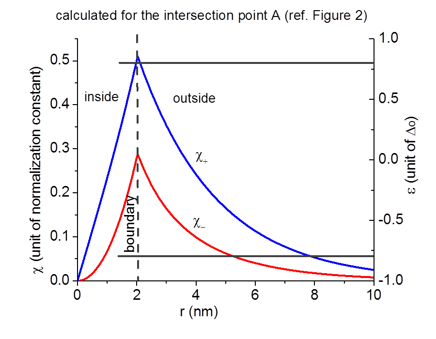
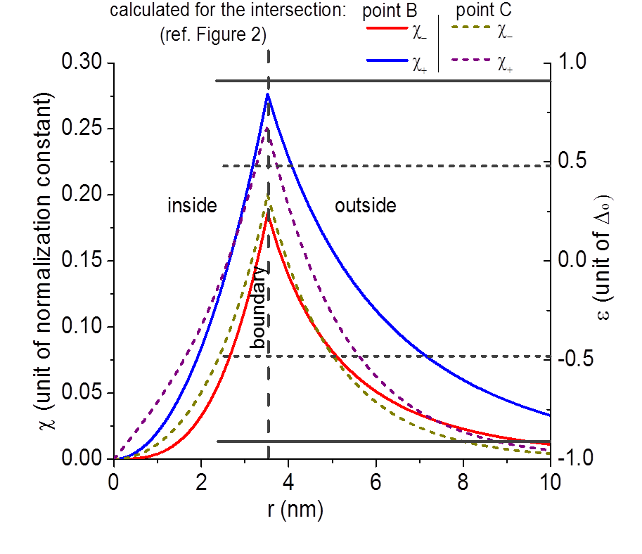
In Figs. 3 and 4 we show the spatial wavefunctions of the $f_{-}$ and $f_{+}$ components inside and outside the QD made of the core-bulk heterostructure PbTe/Pb_0.31Sn_0.69Te. The Fig. 3 shows the example of the intersection point A (see Fig. 2) and the Fig. 4 shows the example of the intersection points B and C (see Fig. 2). Since the 4-spinors must be continuous at the boundary, also each of the 2-spinor components must be continuous, i.e. $f_{-}^{in}=f_{-}^{out}$ and $f_{+}^{in}=f_{+}^{out}$ at the QD surface. The horizontal solid and short dashed lines in Figs. represent the energy eigenvalues, respectively, at the intersection point A, corresponding to $r_{0}=2$ nm, and at the intersection point B and C, corresponding to $r_{0}=3.5$ nm. Eigenvalues are $\varepsilon_{\pm}=\pm 0.80\Delta_{o}$ at point A, $\varepsilon_{\pm}=\pm 0.91\Delta_{o}$ at point B, and $\varepsilon_{\pm}=\pm 0.48\Delta_{o}$ at point C.

In order to show that the solutions correspond to Weyl fermions, we perform an expansion of Eq. (7) for large $z$ to obtain the eigenenergies in the continuum limit. Using the second order in the expansion of the spherical modified Bessel functions for $z\rightarrow\infty$ (see the App. B), we get

This can be written as

which results in the eigenenergies for the electron and hole,

This corresponds to the linear spectrum of free massless Dirac fermions, i.e. free Weyl fermions on a sphere. This means that the energy splittings between the trapped Weyl states in the quantum dot result from the confinement of the Weyl fermions on a sphere. The solution in Eq. (98) corresponds to the eigenspectra found in Ref. 51 for zero magnetic field and without quantum confinement effects.

In the continuum limit, the Nielsen-Ninomiya fermion doubling theorem [52] is satisfied by the pairs of Dirac cones positioned at antipodal points of the sphere defined by the surface of the QD (see App. C for details). However, for a general finite QD radius $r_{o}$ the eigenstates are bound and have a discrete energy spectrum. Since the Nielsen-Ninomiya fermion doubling theorem [52] is valid only for continuum states, it does not apply to the bound Weyl fermions in a 3D TI QD with finite radius $r_{o}$.

The $\mathbf{k}\cdot\mathbf{p}$ Hamiltonian contains also a quadratic term in the momenta,[47] namely

where $m_{\|}^{\mp}$ and $m_{\bot}^{\mp}$ are the longitudinal and transverse effective masses of the $L^{\mp}$ bands, respectively. Through minimal coupling the quadratic term leads to a linear term in the momentum, which we need to take into account. Hence, in the presence of electromagnetic radiation, the total Hamiltonian for the Dirac particle is given by

where $A=(A_{z},\;\boldsymbol{A}_{\perp})$ is the vector potential, $\mathbf{E}=\partial\mathbf{A}/\partial t$ in the Coulomb gauge, and we made use of the equivalence between $(e/m)\mathbf{A}\cdot\mathbf{p}$ and $-e\mathbf{\hat{r}}\cdot\mathbf{E}$.[48] We identify the interaction Hamiltonian as

It will turn out that both interband and intraband transitions contribute. It is important to note that $v_{\|}=P_{\|}/m_{0}$ and $v_{\bot}=P_{\bot}/m_{0}$ include the Kane interband matrix elements $\mathbf{P}=\left\langle u_{\mathbf{k}_{\mathrm{f}}}^{\mp}\left|\mathbf{\hat{P}}\right|u_{\mathbf{k}_{\mathrm{I}}}^{\pm}\right\rangle$, where $u_{\mathbf{k}}^{\mp}$ are the Bloch’s functions for the $L^{\mp}$ bands. This means that the interband transitions are governed by the interband Hamiltonian $H_{inter}=ev_{\|}\alpha_{z}A_{z}+ev_{\bot}\boldsymbol{\alpha}_{\bot}\cdot\boldsymbol{A}_{\bot}$, where the Dirac $\boldsymbol{\alpha}$- matrices couple the $L^{-}$ band with the $L^{+}$ band. The Hamiltonian $H_{intra}=-e\mathbf{\hat{r}}\cdot\mathbf{E}$ accounts for intraband transitions with $\mathbf{\hat{r}}$ operating on the envelope wavefunctions only. $H_{intra}$ is proportional to the identity in 4-spinor space and therefore couples the $L^{-}$ band to itself and the $L^{+}$ band to itself. Thus the interband Hamiltonian $H_{inter}$ and the intraband Hamiltonian $H_{intra}$ are not equivalent in this description. On the one hand, $H_{inter}$ gives rise to interband transitions because it contains the Kane interband matrix elements $P_{\bot}$ and $P_{\|}$. On the other hand, $H_{intra}$ gives rise to intraband transitions because the electric dipole operator $e\mathbf{\hat{r}}$ operates on the envelope wavefunctions. Remarkably, both terms lead to the same strict optical selection rules and add up to a combined optical matrix element, as shown below. This enhancement of the optical matrix element is a feature of the 3D TI QD. In contrast, in a wide-bandgap semiconductor QD the interband and intraband transitions are energetically separated, i.e. interband transitions occur typically around the bandgap energy, whereas intraband transitions occur around the energy level separation due to the confinement of the QD. [46]

Fig. 5 shows the possible transitions between the states $\kappa=1$ and $\kappa=2$. It is to be noted that there is a complete symmetry in the solutions in the sense that a $\kappa$ state can be chosen from either the positive- or the negative-energy solutions.. The optical matrix elements are given by

The incoming photon’s wavelength is much larger than the dot size. Therefore, the transitions are vertical, which means $\mathbf{A}=(A_{x0},A_{y0},A_{z0})e^{i\mathbf{q}\cdot\mathbf{r}}\thickapprox(A_{x0},A_{y0},A_{z0})$ can be used, yielding the electric dipole approximation. The transition energies $\hbar\omega_{0}=\varepsilon_{\kappa=2}-\varepsilon_{\kappa=1}$ are large compared with the room temperature $k_{B}T=25$ meV and the Coulomb charging energy of about 5 meV.[24] For the control of the number of electrons and holes in the 3D TI QD it is necessary to work at low temperatures of around 1 K.

As an example, here we consider transitions between the states $\kappa=1$ (at point C) and $\kappa=2$ (at point B). The matrix elements of the Dirac-$\alpha$ matrix are given by

The matrix elements of $\mathbf{\hat{r}}$ are given by

The spherical harmonics can be determined using the Table 1. In order to obtain optical selection rules for circular polarizations, it is useful to express the scalar products of the interband and the intraband Hamiltonian in the form $\mathbf{e}\cdot\boldsymbol{\alpha}=\mathbf{e}_{z}\alpha_{z}+\mathbf{e}_{-}\alpha_{+}+\mathbf{e}_{+}\alpha_{-}$ and $\mathbf{e}\cdot\mathbf{\hat{r}}=\mathbf{e}_{z}\hat{z}+\mathbf{e}_{-}\hat{r}_{+}+\mathbf{e}_{+}\hat{r}_{-}$, respectively, where $\mathbf{e}_{\pm}=\left(\mathbf{e}_{x}\pm i\mathbf{e}_{y}\right)/\sqrt{2}$ are the unit vectors of circular polarizations, $\alpha_{\pm}=\left(\alpha_{x}\pm i\alpha_{y}\right)/\sqrt{2}$, and $\hat{r}_{\pm}=\left(\hat{x}\pm i\hat{y}\right)/\sqrt{2}=-\sqrt{\frac{4\pi}{3}}rY_{1}^{\pm 1}$. Using our spinor states $\left|\phi_{\mp}\right\rangle$ and radial wavefunction functions $\left|f_{\mp}\right\rangle$ we obtain the following nonzero matrix elements for $\boldsymbol{\alpha}$:

For $\mathbf{\hat{r}}$ we obtain the following nonzero matrix elements:

References

- [1] Moore, J. E. The birth of topological insulators, Nature 464, 194 (2010).
- [2] M. Z. Hasan and C. L. Kane, Rev. Mod. Phys. 82, 3045 (2010).
- [3] Y. L. Chen, J. G. Analytis, J.-H. Chu, Z. K. Liu, S.-K. Mo, X. L. Qi, H. J. Zhang, D. H. Lu, X. Dai, Z. Fang, S. C. Zhang, I. R. Fisher, Z. Hussain & Z.-X. Shen, Science 325, 178-181 (2009).
- [4] D. Hsieh, Y. Xia, L. Wray, D. Qian, A. Pal, J. H. D, J. Osterwalder, F. Meier, G. Bihlmayer, C. L. Kane, Y. S. Hor, R. J. Cava, M. Z. Hasan, Science 323, 919 (2009).
- [5] Y. Xia, D. Qian, D. Hsieh, L. Wray, A. Pal, H. Lin, A. Bansil, D. Grauer, Y. S. Hor, R. J. Cava, M. Z. Hasan, Nature Phys. 5, 398–402 (2009).
- [6] P. Roushan, J. Seo, Colin V. Parker, Y. S. Hor, D. Hsieh, Dong Qian, Anthony Richardella, M. Z. Hasan, R. J. Cava, A. Yazdani, Nature (London) 460, 1106 (2009).
- [7] Z. Alpichshev, J. G. Analytis, J.-H. Chu, I. R. Fisher, Y. L. Chen, Z. X. Shen, A. Fang, A. Kapitulnik, Phys. Rev. Lett. 104, 016401 (2010).
- [8] D. Hsieh, D. Qian, L. Wray, Y. Xia, Y. S. Hor, R. J. Cava, M. Z. Hasan, Nature (London) 452, 970 (2008).
- [9] H. Yusheng, A.D.C. Grassie, J. Phys. F: Met. Phys. 15, 363-376 (1985).
- [10] D. Pesin, A. H. MacDonald, Nature Mater. 11, 409 (2012).
- [11] V. M. Edelstein, Solid State Commun. 73, 233 (1990).
- [12] J. Wunderlich, B. Kaestner, J. Sinova, T. Jungwirth, Phys. Rev. Lett. 94, 047204 (2005).
- [13] C. L. Kane, E. J. Mele, Phys. Rev. Lett. 95, 146802 (2005).
- [14] L. Fu, C. L. Kane, Phys. Rev. B 76, 045302 (2007).
- [15] I. Zutic, J. Fabian, S. Das Sarma, Rev. Mod. Phys. 76, 323-345 (2004).
- [16] D. Hsieh, Y. Xia, D. Qian, L. Wray, J. H. Dil, F. Meier, J. Osterwalder, L. Patthey, J. G. Checkelsky, N. P. Ong, A. V. Fedorov, H. Lin, A. Bansil, D. Grauer, Y. S. Hor, R. J. Cava, M. Z. Hasan, Nature (London) 460, 1101 (2009).
- [17] L. Fu and C. L. Kane, Phys. Rev. Lett. 100, 096407 (2008)
- [18] P. J. Leek, J. M. Fink, A. Blais, R. Bianchetti, M. Göppl, J. M. Gambetta, D. I. Schuster, L. Frunzio, R. J. Schoelkopf, A. Wallraff, Science 318, 1889 (2007).
- [19] H-T. He, G. Wang, T. Zhang, I. K. Sou, G. K. L. Wong, J. N. Wang, H. Z. Lu, S. Q. Shen, F. C. Zhang, Phys. Rev. Lett. 106, 166805 (2011).
- [20] H. Peng, K. Lai, D. Kong, S. Meister, Y. Chen, X.-L. Qi, S.-C. Zhang, Z.-X. Shen, Y. Cui, Nature Mater. 9, 225 (2010).
- [21] J. J. Cha, K. J. Koski, Y. Cui, Phys. Status Solidi (RRL) 7, 15 (2012).
- [22] H. Peng, W. Dang, J. Cao, Y. Chen, D. Wu, W. Zheng, H. L., Z.-X. Shen, Z. Liu, Nature Chem. 4, 218 (2012).
- [23] D. Kong, Y. Cui, Nature Chem. 3, 845 (2011).
- [24] S. Cho, S. Cho, D. Kim , P. Syers, N. P. Butch, J. Paglione, M. S. Fuhrer, Nano Lett. 12, 469 (2012).
- [25] C. Simon, M. Afzelius, J. Appel, A. B. de la Giroday, S. J. Dewhurst, N. Gisin, C. Y. Hu, F. Jelezko, S. Kroll, J. H. Müller, J. Nunn, E. S. Polzik, J. G. Rarity, H. De Riedmatten, W. Rosenfeld, A. J. Shields, N. Skold, R. M. Stevenson, R. Thew, I. A. Walmsley, M. C. Weber, H. Weinfurter, J. Wrachtrup, R. J. Young, Eur. Phys. J. D 58, 1 (2010).
- [26] R. B. Liu, W. Yao, L. J. Sham, Adv. Phys. 59, 703 (2010).
- [27] M. Kroutvar, Y. Ducommun, D. Heiss, M. Bichler, D. Schuh, G. Abstreiter, J. J. Finley, Nature (London) 432, 81 (2004).
- [28] A. Ebbens, D. N. Krizhanovskii, A. I. Tartakovskii, F. Pulizzi, T. Wright, A. V. Savelyev, M. S. Skolnick, M. Hopkinson, Phys. Rev. B 72, 073307 (2005).
- [29] H. J. Krenner, C. E. Pryor, J. He, P. M. Petroff, Nano Lett. 8, 1750 (2008).
- [30] D. Brunner, B. D. Gerardot, P. A. Dalgarno, G. Wust, K. Karrai, N. G. Stoltz, P. M. Petroff, R. J. Warburton, Science 325, 70 (2009).
- [31] M. Atature, J. Dreiser, A. Badolato, A. Imamoglu, Nature Physics 3, 101 (2007).
- [32] A. Imamoglu, D. D. Awschalom, G. Burkard, D. P. DiVincenzo, D. Loss, M. Sherwin, A. Small, Phys. Rev. Lett. 83, 4204 (1999).
- [33] C. Piermarocchi, P. Chen, L. J. Sham, D. G. Steel, Phys. Rev. Lett. 89, 167402 (2002).
- [34] T. Calarco, A. Datta, P. Fedichev, E. Pazy, P. Zoller, Phys. Rev. A 68, 012310 (2003).
- [35] M. Atatüre, J. Dreiser, A. Badolato, A. Högele, K. Karrai, A. Imamoglu, Science 312, 551 (2006).
- [36] B. D. Gerardot, D. Brunner, P. A. Dalgarno, P. Ohberg, S. Seidl, M. Kroner, K. Karrai, N. G. Stoltz, P. M. Petroff, R. J. Warburton, Nature (London) 451, 441 (2008).
- [37] A. N. Vamivakas, C. Y. Lu, C. Matthiesen, Y. Zhao, S. Falt, A. Badolato, M. Atatüre, Nature (London) 467, 297 (2010).
- [38] A. Greilich, D. R. Yakovlev, A. Shabaev, A. L. Efros, I. A. Yugova, R. Oulton, V. Stavarache, D. Reuter, A. Wieck, M. Bayer, Science 313, 341 (2006).
- [39] E. A. Stinaff, M. Scheibner, A. S. Bracker, I. V. Ponomarev, V. L. Korenev, M. E. Ware, M. F. Doty, T. L. Reinecke, D. Gammon, Science 311, 636 (2006).
- [40] L. Robledo, J. Elzerman, G. Jundt, M. Atatüre, A. Högele, S. Fält, A. Imamoglu, Science 320, 772 (2008).
- [41] D. Kim, S. G. Carter, A. Greilich, A. S. Bracker, D. Gammon, Nature Physics 7, 223 (2011).
- [42] A. N. Vamivakas, Y. Zhao, C. Y. Lu, M. Atatüre, Nature Physics 5, 198 (2009).
- [43] M. N. Leuenberger, M. E. Flatté, D. D. Awschalom, Phys. Rev. Lett. 94, 107401 (2005).
- [44] M. N. Leuenberger, Phys. Rev. B 73, 075312 (2006).
- [45] C. Y. Hu, A. Young, J. L. O’Brien, W. J. Munro, J. G. Rarity, Phys. Rev. B 78, 085307 (2008).
- [46] J. Singh, Electronic and Optoelectronic Properties of Semiconductor Structures (Cambridge University Press, Cambridge, 2003).
- [47] G. Nimtz, B. Schlicht, in Narrow Gap Semiconductors (Springer, Berlin, 1983), pp. 45-48.
- [48] J. J. Sakurai, Advanced Quantum Mechanics (Pearson Education, 2007).
- [49] H. P. Paudel and M. N. Leuenberger, preprint: http://arxiv.org/abs/1208.4806.
- [50] B. A. Volkov and Pankratov, JETP Lett. 42, 178 (1985).
- [51] D.-H. Lee, Phys. Rev. Lett. 103, 196804 (2009).
- [52] H. B. Nielsen and M. Ninomiya, Phys. Lett. B 130, 389 (1983); Nuclear Phys. B 185, 20 (1981); Nuclear Phys. B 193, 173 (1981); Phys. Lett. B 105, 219 (1981).
- [53] G. Bastard,Wave Mechanics Applied to Semiconductor Heterostructures (Wiley, New York, 1991).
- [54] E. Rosencher, B. Vinter, Optoelectronics, (Cambridge University Press, Cambridge, 2004).
- [55] H. P. Seigneur, G. González, Michael N. Leuenberger, W. V. Schoenfeld, Adv. OptoElectronics 2011, 893086 (2011).
- [56] G. González, H. P. Seigneur, W. V. Schoenfeld, Michael N. Leuenberger, J. Comput. Theor. Nanosci. 7, 1651 (2010).
- [57] H. P. Seigneur, G. González, Michael N. Leuenberger, W. V. Schoenfeld, Adv. Math. Phys. 2010, 342915 (2010).
- [58] A. V. Thompson, H. P. Seigneur, Michael N. Leuenberger, W. V. Schoenfeld, IEEE J. of Quantum Electronics 45, 637 (2009).
- [59] H. P. Seigneur, Michael N. Leuenberger, W. V. Schoenfeld, J. Appl. Phys. 104, 014307 (2008).
- [60] J. Berezovsky, M. H. Mikkelsen, O. Gywat, N. G. Stoltz, L. A. Coldren & D. D. Awschalom, Science 314, 1916 (2006).
- [61] J. H. Davies, The Physics of Low-dimensional Semiconductors: An Introduction (Cambridge University Press, New York, 1997).
- [62] M. O. Scully, M. S. Zubairy, Quantum Optics (Cambridge Univ. Press, Cambridge, 2001).
- [63] J. P. Reithmaier, G. Sek, A. Loffier, C. Hofmann, S. Kuhn, S. Reitzenstein, L. V. Keldysh, V. D. Kulakovskii, T. L. Reinecke, A. Forchel, Nature (London) 432, 197 (2004).
- [64] M. Abramowitz, I. A. Stegun, Handbook of mathematical functions, p. 443 (Natl. Bur. Std., Washington, 1972).
- [65] T. H. Stievater, X. Li, D. G. Steel, D. Gammon, D. S. Katzer, D. Park, C. Piermarocchi, L. J. Sham, Phys. Rev. Lett. 87, 133603 (2001).
- [66] T. Takagahara, Quantum Coherence, Correlation and Decoherence in Semiconductor Nanostructures (Academic Press, San Diego, 2003).
- [67] M. P. Marder, Condensed Matter Physics (2nd edition, Wiley, New York, 2010).
- [68] R. Shankar, Principles of Quantum Mechanics (2nd edition, Springer, Berlin, 1994).
- [69] M. Veldhorst, M. Snelder, M. Hoek, T. Gang, V. K. Guduru, X. L.Wang, U. Zeitler, W. G. van derWiel, A. A. Golubov, H. Hilgenkamp, A. Brinkman, Nature Mat. 11, 417 (2012).
- [70] M. Nakahara, Geometry, Topology, and Physics (2nd edition, Institute of Physics Publishing, Bristol, 2003).
- [71] J. C. Y. Teo, L. Fu, C. L. Kane, Phys. Rev. B 78, 045426 (2008).
- [72] J. J. Sakurai, Modern Quantum Mechanics (Addison-Wesley, New York, 1994).
- [73] S.-Y. Xu, C. Liu, N. Alidoust, M. Neupane, D. Qian, I. Belopolski, J. D. Denlinger, Y. J. Wang, H. Lin, L. A. Wray, G. Landolt, B. Slomski, J. H. Dil, A. Marcinkova, E. Morosan, Q. Gibson, R. Sankar, F. C. Chou, R. J. Cava, A. Bansil, M. Z. Hasan, Nature Comm. 3, 1192 (2012).
- [74] P. Y. Yu and M. Cardona, Fundamentals of Semiconductors: Physics and Material Properties (3rd edition, Springer, Berlin, 2005).
- [75] M. Fox, Quantum Optics: An Introduction (Oxford University Press, 2006).