跳到论文正文
W Papers独立论文阅读器 arXiv:1212.6450 论文正文 计算阅读时间 · 0%
引用这篇论文根据当前论文元数据生成,正式投稿前建议核对。


License: arXiv.org perpetual non-exclusive license
arXiv:1212.6450v1 [math.OC] 28 Dec 2012

Reach Control on Simplices by Piecewise Affine Feedback

Mireille E. Broucke and Marcus Ganness Address: Dept. of Electrical and Computer Engineering
University of Toronto, Toronto ON Canada M5S 3G4
Email address: broucke@control.utoronto.ca
Date: August 24, 2026
Abstract.

We study the reach control problem for affine systems on simplices, and the focus is on cases when it is known that the problem is not solvable by continuous state feedback. We examine from a geometric viewpoint the structural properties of the system which make continuous state feedbacks fail. This structure is encoded by so-called reach control indices, which are defined and developed in the paper. Based on these indices, we propose a subdivision algorithm and associated piecewise affine feedback. The method is shown to solve the reach control problem in all remaining cases, assuming it is solvable by open-loop controls.

1. Introduction

This paper studies the reach control problem (RCP) on simplices. The problem is for trajectories of an affine system defined on a simplex to reach a prespecified facet of the simplex in finite time. The overall concept of the problem and its setting were introduced in [15] and further developed in [16, 17, 26, 7]. The significance of the problem stems from its capturing the essential features of reachability problems for control systems: the presence of state constraints and the notion of trajectories reaching a goal in a guided and finite-time manner. The problem fits within a larger family of reachability problems; namely, to reach a target set 𝒳f\mathcal{X}_{f} with state constraint in a set 𝒳\mathcal{X}, denoted as 𝒳​⟶𝒳​𝒳f\mathcal{X}\overset{\mathcal{X}}{\longrightarrow}\mathcal{X}_{f}. In the present context, we assume that the state constraints give rise to a state space that is triangulable [18]; then the reachability specification is converted to a sequence of reachability problems on simplices of the triangulation. The reader is referred to [7, 15, 16, 17, 26, 21, 2] for further motivations, including how the studied problem arises in fundamental problems concerning hybrid systems [14].

RCP is one among several different research paths for analysis and synthesis of piecewise affine (PWA) feedback [4, 11, 27]. Recent progress on explicit MPC schemes has fueled the interest in PWA feedbacks [4], such feedbacks play a prominent role in linear switched systems [19], and PWA systems have significant applications in engineering and biology [28, 12, 23, 20]. A feature of our approach is that, rather than directly computing a controller numerically, we seek conditions for existence of controllers based on the problem data. This follows classical lines of thought which are well established in control theory. Another classical underpinning is to exploit system structure to understand the limits of a control system, again distinguishing our approach from numerical methods.

2. Contributions

In [7] it was shown that, under a suitable triangulation of the state space, affine feedback and continuous state feedback are equivalent from the point of view of solvability of the reach control problem (RCP). The approach is based, fundamentally, on fixed point theory. The latter allows to deduce that continuous state feedbacks always generate closed-loop equilibria inside the simplex when affine feedbacks do. The current paper departs from these findings, and using a geometric approach, we explore the system structure that gives rise to equilibria. This structure is encoded in so-called reach control indices. The first goal of this paper is to elucidate these indices. The second goal is to use the indices to obtain a subdivision of the simplex and an associated piecewise affine feedback to solve RCP in those cases when the problem is not solvable by continuous state feedback. It is shown that RCP is solvable by piecewise affine feedback if it is solvable by open-loop controls. This finding gives strong evidence to the relevance of the class of piecewise affine feedbacks in solving reachability problems.

Refer to caption
Figure 1. Main idea in a 2D example.

The main ideas of the paper can be understood informally. Consider a 2D simplex 𝒮=co​{v0,v1,v2}{\mathcal{S}}=\textup{co}\{v_{0},v_{1},v_{2}\} the convex hull of vertices v0v_{0}, v1v_{1}, and v2v_{2}, with 1D facets ℱ0{\mathcal{F}}_{0}, ℱ1{\mathcal{F}}_{1}, and ℱ2{\mathcal{F}}_{2}, as in Figure 1(a). Consider a single-input control system x˙=A​x+b​u+a\dot{x}=Ax+bu+a defined on 𝒮{\mathcal{S}}. The reach control problem is to find a state feedback u=f⁡(x)u=f(x) such that all closed-loop trajectories initialized in 𝒮{\mathcal{S}} leave 𝒮{\mathcal{S}} in finite time through the exit facet ℱ0{\mathcal{F}}_{0}. The procedure to solve this control problem by continuous state feedback is to select control values uiu_{i} at the vertices viv_{i} such that the velocity vectors A​vi+b​ui+aAv_{i}+bu_{i}+a point inside cone​(𝒮)\textup{cone}({\mathcal{S}}), the cone with apex at v0v_{0} determined by 𝒮{\mathcal{S}}; otherwise trajectories may leave 𝒮{\mathcal{S}} through ℱ1{\mathcal{F}}_{1} or ℱ2{\mathcal{F}}_{2}, which is disallowed. The controller u=f⁡(x)u=f(x) is formed as a continuous interpolation of the control values at the vertices. Label the vertex velocity vectors as y0=A​v0+b​u0+ay_{0}=Av_{0}+bu_{0}+a, and bi=A​vi+b​ui+ab_{i}=Av_{i}+bu_{i}+a, i=1,2i=1,2, as in the figure. Suppose that A​x+a∈Im​(b)Ax+a\in\textup{Im}(b) along a line 𝒪{\mathcal{O}} through v1v_{1} and v2v_{2}. Clearly closed loop equilibria can only appear on the set 𝒢:=𝒮∩𝒪{\mathcal{G}}:={\mathcal{S}}\cap{\mathcal{O}}. Now it is obvious that this control problem cannot be solved by any continuous state feedback. For at v1v_{1}, b1b_{1} has to point down to be inside cone​(𝒮)\textup{cone}({\mathcal{S}}), but at v2v_{2}, b2b_{2} has to point up. If we continuously interpolate along ℱ0{\mathcal{F}}_{0} from v1v_{1} to v2v_{2}, the continuous vector field, always in Im​(b)\textup{Im}(b) along ℱ0{\mathcal{F}}_{0}, must pass through zero (by the Intermediate Value Theorem) at some x¯\overline{x} along ℱ0{\mathcal{F}}_{0}. The defect is that there are two vertices v1v_{1} and v2v_{2} that “share” the only control direction available, bb.

Suppose we now allow discontinuous feedback. Place a point v′v^{\prime} along the edge from v0v_{0} to v1v_{1} and define a new simplex 𝒮1=co​{v′,v1,v2}{\mathcal{S}}^{1}=\textup{co}\{v^{\prime},v_{1},v_{2}\}. See Figure 1(b). Notice that as we slide v′v^{\prime} from v0v_{0} to v1v_{1} the cone cone​(𝒮1)\textup{cone}({\mathcal{S}}^{1}) with apex at v′v^{\prime} widens at v2v_{2} enough that −b2-b_{2} points inside cone​(𝒮1)\textup{cone}({\mathcal{S}}^{1}) at v2v_{2}. Notice also that v1v_{1} is unaffected by sliding v′v^{\prime}. Pick such a v′v^{\prime}. Then one can construct an affine feedback u=K1​x+g1u=K^{1}x+g^{1} on 𝒮1{\mathcal{S}}^{1} that assigns a non-zero velocity vector at every point on ℱ0{\mathcal{F}}_{0}, so there is no closed loop equilibrium in 𝒮1{\mathcal{S}}^{1}. By [17, 26], RCP is solved on 𝒮1{\mathcal{S}}^{1}. For the remaining simplex 𝒮2{\mathcal{S}}^{2} it is also possible to devise an affine controller so there is no equilibrium in 𝒮2{\mathcal{S}}^{2}. This is because equilibria can only appear in 𝒮2{\mathcal{S}}^{2} at v2∈𝒪v_{2}\in{\mathcal{O}}. But at v2v_{2} we can select the velocity vector b2≠0b_{2}\neq 0. Again RCP can be solved on 𝒮2{\mathcal{S}}^{2} by affine feedback. Combining the two affine feedbacks, we get a discontinuous piecewise affine feedback that solves RCP on 𝒮{\mathcal{S}}. Note that a discontinuity is introduced because we use two different control values at v2v_{2}.

The contribution of the paper is to make mathematically rigorous the informal ideas described above. The main technical difficulty arises in dealing with multi-input systems. For this we bring in two tools. First we introduce the reach control indices to group together vertices in 𝒢{\mathcal{G}} that share control inputs. These indices are similar in spirit to the controllability indices to group together states that share control inputs [10]. As with the controllability indices, the reach control indices require a special ordering of a set of linearly independent vectors; however, other technical details are different. The second tool is ℳ{\mathscr{M}}-matrices which help to concisely represent the constraints on the vector field at vertices of 𝒢{\mathcal{G}}. The reader is referred to Chapter 6 of [5] for relevant background.

The paper is organized as follows. In Section 3 we review the reach control problem. In Section 4 we give necessary conditions for solvability by open-loop controls. These then shape the assumptions to construct the reach control indices, which are developed in Section 5. In Section 6, a subdivision method and associated piecewise affine feedback are proposed to solve RCP when continuous state feedback does not. The main result is presented in Section 6 showing the relationship between solvability via open-loop controls and solvability via piecewise affine feeback. Examples are presented in Section 7. Preliminary versions of parts of this paper appeared in [8, 9]. Proofs of supporting lemmas are found in the Appendix.

Notation. For x∈ℝnx\in{\mathbb{R}}^{n}, the notation x≻0x\succ 0 (x⪰0x\succeq 0) means xi>0x_{i}>0 (xi≥0x_{i}\geq 0) for 1≤i≤n1\leq i\leq n. The notation x≺0x\prec 0 (x⪯0x\preceq 0) means −x≻0-x\succ 0 (−x⪰0-x\succeq 0). Notation 𝟎{\mathbf{0}} denotes the subset of ℝn{\mathbb{R}}^{n} containing only the zero vector. The notation ℬ{\mathscr{B}} denotes the open unit ball, and ℬ¯\overline{{\mathscr{B}}} denotes its closure. The notation co​{v1,v2,…}\textup{co}\{v_{1},v_{2},\ldots\} denotes the convex hull of a set of points vi∈ℝnv_{i}\in{\mathbb{R}}^{n}, and sp​{y1,y2,…}\textup{sp}\{y_{1},y_{2},\ldots\} denotes the span of vectors yi∈ℝny_{i}\in{\mathbb{R}}^{n}. The notation (vi,vj)(v_{i},v_{j}) denotes the open segment in ℝn{\mathbb{R}}^{n} between vi,vj∈ℝnv_{i},v_{j}\in{\mathbb{R}}^{n}. Finally, T𝒮​(x)T_{{\mathcal{S}}}(x) denotes the Bouligand tangent cone to set 𝒮{\mathcal{S}} at a point xx [13].

3. Problem Statement

Consider an nn-dimensional simplex 𝒮{\mathcal{S}}, the convex hull of n+1n+1 affinely independent points in ℝn{\mathbb{R}}^{n}. Let its vertex set be V:={v0,…,vn}V:=\{v_{0},\dots,v_{n}\} and its facets ℱ0,…,ℱn\mathcal{F}_{0},\dots,\mathcal{F}_{n}. The facet will be indexed by the vertex it does not contain. Let hj∈ℝnh_{j}\in{\mathbb{R}}^{n}, j=0,…,nj=0,\dots,n be the unit normal vector to each facet ℱj\mathcal{F}_{j} pointing outside of the simplex. Facet ℱ0\mathcal{F}_{0} is called the exit facet of 𝒮\mathcal{S}. Define the index set I:={1,…,n}I:=\{1,\ldots,n\}. For x∈𝒮x\in{\mathcal{S}} defined the closed, convex cone

𝒞(x):={y∈ℝn|hj⋅y≤0,j∈Is.t.x∈ℱj}.{\mathcal{C}}(x):=\{y\in{\mathbb{R}}^{n}~|~h_{j}\cdot y\leq 0,~j\in I~~s.t.~~x\in{\mathcal{F}}_{j}\}\,.

We’ll write cone​(𝒮):=𝒞​(v0)\textup{cone}({\mathcal{S}}):={\mathcal{C}}(v_{0}) because 𝒞⁡(v0){\mathcal{C}}(v_{0}) is the tangent cone to 𝒮{\mathcal{S}} at v0v_{0}. We consider the affine control system on 𝒮{\mathcal{S}}:

x˙=A​x+B​u+a,\dot{x}=Ax+Bu+a\,, (1)

where A∈ℝn×nA\in\mathbb{R}^{n\times n}, a∈ℝna\in\mathbb{R}^{n}, B∈ℝn×mB\in\mathbb{R}^{n\times m}, and rank​(B)=m\textup{rank}(B)=m. Let ℬ=Im​(B)\mathcal{B}=\textup{Im}(B), the image of BB. Define 𝒪:={x∈ℝn|A​x+a∈ℬ}{\mathcal{O}}:=\{~x\in{\mathbb{R}}^{n}~|~Ax+a\in{\mathcal{B}}\} and 𝒢:=𝒮∩𝒪{\mathcal{G}}:={\mathcal{S}}\cap{\mathcal{O}}. Note that closed-loop equilibria of (1) can only appear in 𝒪{\mathcal{O}}. Let ϕu​(t,x0)\phi_{u}(t,x_{0}) denote the trajectory of (1) starting at x0x_{0} under input uu.

Example 1.

Consider Figure 2 where we illustrate the notation in a 2D example. We have a full-dimensional simplex in ℝ2{\mathbb{R}}^{2} given by 𝒮=co​{v0,v1,v2}{\mathcal{S}}=\textup{co}\{v_{0},v_{1},v_{2}\} with vertex set V={v0,v1,v2}V=\{v_{0},v_{1},v_{2}\} and facets ℱ0{\mathcal{F}}_{0},ℱ1{\mathcal{F}}_{1}, and ℱ2{\mathcal{F}}_{2}. Each facet ℱj{\mathcal{F}}_{j} has an outward normal vector hjh_{j}. The only vertex not in facet ℱj{\mathcal{F}}_{j} is vertex vjv_{j}. ℱ0{\mathcal{F}}_{0} is the exit facet. If we assume that v0=0v_{0}=0, then subspace ℬ{\mathcal{B}} is shown passing through v0v_{0}. The set 𝒪{\mathcal{O}} is an affine space shown passing through ℱ0{\mathcal{F}}_{0}. Notice in this case 𝒢=𝒮∩𝒪=co​{v1,v2}{\mathcal{G}}={\mathcal{S}}\cap{\mathcal{O}}=\textup{co}\{v_{1},v_{2}\}. The cone cone​(𝒮)\textup{cone}({\mathcal{S}}) is the cone with apex at v0v_{0} determined by 𝒮{\mathcal{S}}. It is indicated in the figure as the shaded area. The cones 𝒞⁡(vi){\mathcal{C}}(v_{i}), i=0,1,2i=0,1,2 are depicted as darker shaded cones attached at each vertex. Of course, the apex of each 𝒞⁡(vi){\mathcal{C}}(v_{i}) is at the origin, but we depict it as being attached at the corresponding vertex viv_{i} since it will be used to describe allowable directions for the vector field at the vertices. Notice that the cones 𝒞⁡(v1){\mathcal{C}}(v_{1}) and 𝒞⁡(v2){\mathcal{C}}(v_{2}) are not tangent cones to 𝒮{\mathcal{S}} at v1v_{1} and v2v_{2}, respectively, whereas 𝒞⁡(v0){\mathcal{C}}(v_{0}) is the tangent cone to 𝒮{\mathcal{S}} at v0v_{0}; hence the distinguished labeling of 𝒞⁡(v0){\mathcal{C}}(v_{0}) as cone​(𝒮)\textup{cone}({\mathcal{S}}).

Refer to caption
Figure 2. Notation for reach control problem.

We are interested in formulating a problem to make the closed-loop trajectories of (1) exit 𝒮{\mathcal{S}} through the exit facet ℱ0{\mathcal{F}}_{0} only. For this, we require conditions that disallow trajectories to exit from any other facet ℱi{\mathcal{F}}_{i}, i∈Ii\in I. We say the invariance conditions are solvable at vertex vi∈Vv_{i}\in V if there exists ui∈ℝmu_{i}\in{\mathbb{R}}^{m} such that

A​vi+B​ui+a∈𝒞⁡(vi).Av_{i}+Bu_{i}+a\in{\mathcal{C}}(v_{i})\,. (2)

We say the invariance conditions are solvable if (2) is solvable at each vi∈Vv_{i}\in V. The inequalities (2) are called invariance conditions. They guarantee trajectories cannot exit from the facets ℱi{\mathcal{F}}_{i}, i∈Ii\in I, and they are used to construct affine feedbacks [16]. For general state feedbacks, stronger conditions (also called invariance conditions) are needed. We say a state feedback u=f⁡(x)u=f(x) satisfies the invariance conditions if for all x∈𝒮x\in{\mathcal{S}},

A​x+B​f​(x)+a∈𝒞⁡(x).Ax+Bf(x)+a\in{\mathcal{C}}(x)\,. (3)
Example 2.

Consider Figure 3. Attached at each vertex is a velocity vector yi:=A​vi+B​ui+ay_{i}:=Av_{i}+Bu_{i}+a, i∈{0}∪Ii\in\{0\}\cup I. The invariance conditions (2) require that yi∈𝒞⁡(vi)y_{i}\in{\mathcal{C}}(v_{i}), as illustrated. Notice that velocity vectors at vi∈ℱ0v_{i}\in{\mathcal{F}}_{0} may or may not point out of 𝒮{\mathcal{S}}. If the control is an affine feedback u=K​x+gu=Kx+g such that ui=K​vi+gu_{i}=Kv_{i}+g, then by convexity of the closed-loop vector field, (3) holds at every x∈ℱix\in{\mathcal{F}}_{i}, i∈Ii\in I. If the input is a continuous state feedback u=f⁡(x)u=f(x), then invariance conditions for every x∈ℱix\in{\mathcal{F}}_{i}, i∈Ii\in I, must be explicitly stated, since convexity is not guaranteed; hence (3).

Refer to caption
Figure 3. The invariance conditions state that yi:=A​vi+B​ui+a∈𝒞⁡(vi)y_{i}:=Av_{i}+Bu_{i}+a\in{\mathcal{C}}(v_{i}) for i=0,…,ni=0,\ldots,n.
Problem 1 (Reach Control Problem (RCP)).

Consider system (1) defined on 𝒮\mathcal{S}. Find a state feedback u=f⁡(x)u=f(x) such that:

  1. (i)

    For every x∈𝒮x\in{\mathcal{S}} there exist T≥0T\geq 0 and γ>0\gamma>0 such that ϕu​(t,x)∈𝒮\phi_{u}(t,x)\in{\mathcal{S}} for all t∈[0,T]t\in[0,T], ϕu​(T,x)∈ℱ0\phi_{u}(T,x)\in{\mathcal{F}}_{0}, and ϕu​(t,x)∉𝒮\phi_{u}(t,x)\notin{\mathcal{S}} for all t∈(T,T+γ)t\in(T,T+\gamma).

  2. (ii)

    There exists ε>0\varepsilon>0 such that for every x∈𝒮x\in{\mathcal{S}}, ‖A​x+B​f​(x)+a‖>ε~~\|Ax+Bf(x)+a\|>\varepsilon.

  3. (iii)

    Feedback u=f⁡(x)u=f(x) satisfies the invariance conditions (3).

Condition (i) is the same condition that appears in the standard formulation of RCP [17, 26]. It states that all closed-loop trajectories must exit 𝒮{\mathcal{S}} through ℱ0{\mathcal{F}}_{0} in finite time without first exiting from another facet. Condition (ii) and (iii) are new, and they are introduced to deal with pathologies that can only happen when using discontinuous feedbacks. It can be shown that if continuous state feedback is used, then condition (i) implies conditions (ii) and (iii) [16]. Therefore, results on affine feedbacks [17, 26] and continuous state feedbacks [7] remain valid.

Example 3.

In this example we illustrate the need for condition (ii). Figure 4(a) illustrates a 2D simplex 𝒮=co​{v0,v1,v2}{\mathcal{S}}=\textup{co}\{v_{0},v_{1},v_{2}\}, where v0=(1,1)v_{0}=(1,1), v1=(0,0)v_{1}=(0,0), and v2=(2,0)v_{2}=(2,0). We consider the linear system on 𝒮{\mathcal{S}}:

x˙=[2−21−2]​x+[21]​u.\dot{x}=\left[\begin{array}[]{rr}2&-2\\ 1&-2\end{array}\right]x+\left[\begin{array}[]{r}2\\ 1\end{array}\right]u\,.

Now we select control values u0=0u_{0}=0, u1=0u_{1}=0, and u2=−3u_{2}=-3 to satisfy the invariance conditions of 𝒮{\mathcal{S}}, and we solve for the feedback u=−32​x1+32​x2u=-\frac{3}{2}x_{1}+\frac{3}{2}x_{2}. The closed loop system has an equilibrium in 𝒮{\mathcal{S}} at v1v_{1} only, and if we compute the time to reach ℱ0{\mathcal{F}}_{0} from any x0∈𝒮x_{0}\in{\mathcal{S}} we find it is finite, despite the presence of the equilibrium. Now we define a discontinuous piecewise affine feedback u=f⁡(x)u=f(x) given by f⁡(x):=−32​x1+32​x2f(x):=-\frac{3}{2}x_{1}+\frac{3}{2}x_{2} for x∈𝒮∖{v1}x\in{\mathcal{S}}\setminus\{v_{1}\} and f⁡(v1):=−1f(v_{1}):=-1. Not only do all trajectories reach ℱ0{\mathcal{F}}_{0} in finite time, they also exit 𝒮{\mathcal{S}} as required by condition (i). We have a feasible solution to RCP, but it is not structurally stable. If the system parameters (A,B,a)(A,B,a) are slightly perturbed and we use u=f⁡(x)u=f(x), then there can appear an equilibrium x¯\overline{x} of the perturbed system in the interior of 𝒮{\mathcal{S}}, as shown in Figure 4(b). Thus, RCP is not solved for the perturbed system. Condition (ii) disallows such non-robust solutions.

Example 4.

Next consider Figure 4(c) which represents a second pathological solution to RCP using discontinuous feedback. Here trajectories reach ℱ0{\mathcal{F}}_{0} in finite time, and then they slide along ℱ0{\mathcal{F}}_{0} out of the simplex along a direction at v2v_{2} that violates v2v_{2}’s invariance conditions. In order to circumvent this behavior, it is sufficient to disallow feedbacks that violate the invariance conditions (3), particularly on ℱ0{\mathcal{F}}_{0}. This is the purpose of condition (iii).

In the sequel we will use the shorthand notation 𝒮​⟶𝒮​ℱ0{\mathcal{S}}\overset{{\mathcal{S}}}{\longrightarrow}{\mathcal{F}}_{0} to denote that (i)-(iii) of Problem 1 hold under some control law. Finally, we make an important assumption concerning the placement of 𝒪{\mathcal{O}} with respect to 𝒮{\mathcal{S}}. The reader is referred to [7] for the motivation and a method of triangulation of the state space that achieves this assumption. See also [18].

Assumption 5.

Simplex 𝒮{\mathcal{S}} and system (1) satisfy the following condition: if 𝒢≠∅{\mathcal{G}}\neq\emptyset, then 𝒢{\mathcal{G}} is a κ\kappa-dimensional face of 𝒮{\mathcal{S}}, where 0≤κ≤n0\leq\kappa\leq n.

Refer to caption
Figure 4. Illustration of pathologies that arise using discontinuous feedback to solve RCP.

4. Necessary Conditions

In this section we present two necessary conditions for solvability of RCP using open-loop controls. We take as open-loop controls for (1) any measurable function μ:[0,∞)→ℝm\mu:[0,\infty)\rightarrow{\mathbb{R}}^{m} that is bounded on compact intervals. Now we define what is meant by a solution of RCP by open-loop controls.

Definition 6.

Consider system (1) defined on 𝒮\mathcal{S}. We say 𝒮​⟶𝒮​ℱ0{\mathcal{S}}\overset{{\mathcal{S}}}{\longrightarrow}{\mathcal{F}}_{0} by open-loop controls if there exists a map T:𝒮→ℝ+T:{\mathcal{S}}\rightarrow{\mathbb{R}}^{+} and a set of open-loop controls {μx|x∈𝒮}\{\mu_{x}~|~x\in{\mathcal{S}}\} such that:

  1. (i)

    For every x∈𝒮x\in\mathcal{S} there exists γ>0\gamma>0 such that ϕμx​(t,x)∈𝒮\phi_{\mu_{x}}(t,x)\in\mathcal{S} for all t∈[0,T⁡(x)]t\in[0,T(x)], ϕμx​(T⁡(x),x)∈ℱ0\phi_{\mu_{x}}(T(x),x)\in\mathcal{F}_{0}, and ϕμx​(t,x)∉𝒮\phi_{\mu_{x}}(t,x)\notin\mathcal{S} for all t∈(T⁡(x),T⁡(x)+γ)t\in(T(x),T(x)+\gamma).

  2. (ii)

    There exists ε>0\varepsilon>0 such that for every x∈𝒮x\in{\mathcal{S}} and t∈[0,T⁡(x)]t\in[0,T(x)], ‖A​ϕμx​(t,x)+B​μx​(t)+a‖>ε\|A\phi_{\mu_{x}}(t,x)+B\mu_{x}(t)+a\|>\varepsilon.

  3. (iii)

    For every x∈𝒮x\in{\mathcal{S}} and t∈[0,T⁡(x)]t\in[0,T(x)], (A​ϕμx​(t,x)+B​μx​(t)+a)∈𝒞⁡((ϕμx​(t,x)))(A\phi_{\mu_{x}}(t,x)+B\mu_{x}(t)+a)\in{\mathcal{C}}({\left(\phi_{\mu_{x}}(t,x)\right)}).

The first result of the section is that solvability of the invariance conditions (2) is necessary for solvability of RCP by open-loop controls in the sense of condition (i) only. This extends the analogous result in [16] on the necessity of the invariance conditions for solvability of RCP (in the sense of condition (i) only) for continuous state feedbacks. Proofs are in the Appendix.

Theorem 7.

If 𝒮​⟶𝒮​ℱ0{\mathcal{S}}\overset{{\mathcal{S}}}{\longrightarrow}{\mathcal{F}}_{0} by open-loop controls in the sense of condition (i) only, then the invariance conditions (2) are solvable.

The second result says that if RCP is solvable by open-loop controls, then it is possible to assign non-zero velocity vectors satisfying (2) at vertices vi∈V∩𝒢v_{i}\in V\cap{\mathcal{G}}. This is an immediate consequence of condition (ii). We know that A​vi+a∈ℬAv_{i}+a\in{\mathcal{B}} for vertices vi∈𝒢v_{i}\in{\mathcal{G}}. Theorem 7 says that if RCP is solvable by open-loop controls (in the sense of condition (i)), then ℬ∩𝒞⁡(vi)≠∅{\mathcal{B}}\cap{\mathcal{C}}(v_{i})\neq\emptyset, for vi∈V∩𝒢v_{i}\in V\cap{\mathcal{G}}. The next result says that, moreover, the zero vector cannot be the only element of ℬ∩𝒞⁡(vi){\mathcal{B}}\cap{\mathcal{C}}(v_{i}), vi∈V∩𝒢v_{i}\in V\cap{\mathcal{G}}.

Theorem 8.

If 𝒮​⟶𝒮​ℱ0{\mathcal{S}}\overset{{\mathcal{S}}}{\longrightarrow}{\mathcal{F}}_{0} by open-loop controls, then ℬ∩𝒞⁡(vi)≠𝟎{\mathcal{B}}\cap{\mathcal{C}}(v_{i})\neq{\mathbf{0}}, vi∈V∩𝒢v_{i}\in V\cap{\mathcal{G}}.

5. Reach Control Indices

The reach control indices are defined in the situation when it is known that RCP is not solvable by continuous state feedback but it is still solvable by open-loop controls. According to the results of [7], RCP is not solvable by continuous state feedback under the following assumptions.

Assumption 9.

Simplex 𝒮{\mathcal{S}} and system (1) satisfy the following conditions.

  1. (A1)

    𝒢=𝒮∩𝒪=co​{v1,…,vκ+1}{\mathcal{G}}={\mathcal{S}}\cap{\mathcal{O}}=\textup{co}\{v_{1},\ldots,v_{\kappa+1}\}, with 0≤κ<n0\leq\kappa<n.

  2. (A2)

    ℬ∩cone​(𝒮)=𝟎{\mathcal{B}}\cap\textup{cone}({\mathcal{S}})={\mathbf{0}}.

  3. (A3)

    The maximum number of linearly independent vectors in any set {b1,…,bκ+1|bi∈ℬ∩𝒞(vi)}\{b_{1},\ldots,b_{\kappa+1}~|~b_{i}\in{\mathcal{B}}\cap{\mathcal{C}}(v_{i})\} (with only one vector for each ℬ∩𝒞⁡(vi){\mathcal{B}}\cap{\mathcal{C}}(v_{i})) is m^\widehat{m} with 0≤m^<κ+10\leq\widehat{m}<\kappa+1.

  4. (A4)

    ℬ∩𝒞⁡(vi)≠𝟎{\mathcal{B}}\cap{\mathcal{C}}(v_{i})\neq{\mathbf{0}}, i=1,…,κ+1i=1,\ldots,\kappa+1.

Assumption (A1) restricts 𝒢{\mathcal{G}} to be a face in ℱ0{\mathcal{F}}_{0}. The other cases arising under Assumption 5 when 𝒢=∅{\mathcal{G}}=\emptyset or v0∈𝒢v_{0}\in{\mathcal{G}} are trivially solvable (Theorems 6.1 and Remark 7.1 of [7]). If either (A2) or (A3) does not hold, then RCP is solved by affine feedback (Theorems 6.2 and 6.7 of [7]). Assumption (A4) is no loss of generality due to Theorem 8.

Example 10.

Consider Figure 2. We have 𝒢=co​{v1,v2}{\mathcal{G}}=\textup{co}\{v_{1},v_{2}\}, which satisfies (A1). Notice (A1) is a strengthening of Assumption 5 - it imposes that v0∉𝒢v_{0}\not\in{\mathcal{G}}; otherwise RCP is not solvable [7]. (A2) is also illustrated in Figure 2. At v0v_{0}, ℬ{\mathcal{B}} has no vectors in common with cone​(𝒮)\textup{cone}({\mathcal{S}}) except the zero vector. Next, we see that (A3) is satisfied with m^=m=1\widehat{m}=m=1. In particular, b1∈ℬ∩𝒞⁡(v1)b_{1}\in{\mathcal{B}}\cap{\mathcal{C}}(v_{1}) and b2∈ℬ∩𝒞⁡(v2)b_{2}\in{\mathcal{B}}\cap{\mathcal{C}}(v_{2}) are linearly dependent. Note also that (A3) specifies that m^<κ+1\widehat{m}<\kappa+1. If m^=κ+1\widehat{m}=\kappa+1, then RCP is solvable by affine feedback [7]. Finally (A4) is taken from Theorem 8. It says that at each vertex in 𝒢{\mathcal{G}}, there exists a non-zero bi∈ℬb_{i}\in{\mathcal{B}} satisfying the invariance conditions of viv_{i} for i=1,2i=1,2.

Consider (A3). Select any bi∈ℬ∩𝒞⁡(vi)b_{i}\in{\mathcal{B}}\cap{\mathcal{C}}(v_{i}), i=1,…,κ+1i=1,\ldots,\kappa+1 and write the list {b1,…,bκ+1}\{b_{1},\ldots,b_{\kappa+1}\}. Clearly there exists a list with a maximum number m^\widehat{m} of linearly independent vectors. W.l.o.g., we reorder the indices {1,…,κ+1}\{1,\ldots,\kappa+1\} (leaving the indices 0,κ+2,…,n0,\kappa+2,\ldots,n the same) so that {b1,…,bm^}\{b_{1},\ldots,b_{\widehat{m}}\} are linearly independent. By (A3), m^<κ+1\widehat{m}<\kappa+1 so we can define p≥1p\geq 1 as

p:=κ+1−m^.p:=\kappa+1-\widehat{m}\,.

Notice by the maximality of {b1,…,bm^}\{b_{1},\ldots,b_{\widehat{m}}\}, for each i=m^+1,…,κ+1i=\widehat{m}+1,\ldots,\kappa+1 and for each bi∈ℬ∩𝒞⁡(vi)b_{i}\in{\mathcal{B}}\cap{\mathcal{C}}(v_{i}), bi∈sp​{b1,…,bm^}b_{i}\in\textup{sp}\{b_{1},\ldots,b_{\widehat{m}}\}. Now consider the cone ℬ∩𝒞⁡(vm^+1){\mathcal{B}}\cap{\mathcal{C}}(v_{\widehat{m}+1}). By (A4), ℬ∩𝒞⁡(vm^+1)≠𝟎{\mathcal{B}}\cap{\mathcal{C}}(v_{\widehat{m}+1})\neq{\mathbf{0}}, so there exists 2≤r1≤m^+12\leq r_{1}\leq\widehat{m}+1 such that w.l.o.g. (reordering indices 1,…,m^1,\ldots,\widehat{m}), ℬ∩𝒞⁡(vm^+1)⊂sp​{b1,…,br1−1}{\mathcal{B}}\cap{\mathcal{C}}(v_{\widehat{m}+1})\subset\textup{sp}\{b_{1},\ldots,b_{r_{1}-1}\} and sp​{b1,…,br1−1}\textup{sp}\{b_{1},\ldots,b_{r_{1}-1}\} is the smallest subspace generated by basis vectors among {b1,…,bm^}\{b_{1},\ldots,b_{\widehat{m}}\} only that contains the cone ℬ∩𝒞⁡(vm^+1){\mathcal{B}}\cap{\mathcal{C}}(v_{\widehat{m}+1}).

Lemma 11.

There exists a unique minimal subspace containing ℬ∩𝒞⁡(vm^+1){\mathcal{B}}\cap{\mathcal{C}}(v_{\widehat{m}+1}) and generated by the basis {b1,…,bm^}\{b_{1},\ldots,b_{\widehat{m}}\}.

In order to have consecutive indices, it is useful to renumber the vertices of 𝒢{\mathcal{G}} to effectively swap the indices m^+1\widehat{m}+1 and r1r_{1}, so we get

ℬ∩𝒞⁡(vr1)⊂sp​{b1,…,br1−1}.{\mathcal{B}}\cap{\mathcal{C}}(v_{r_{1}})\subset\textup{sp}\{b_{1},\ldots,b_{r_{1}-1}\}\,. (4)

The following establishes that one can always find a vector in ℬ∩𝒞⁡(vr1){\mathcal{B}}\cap{\mathcal{C}}(v_{r_{1}}) that depends on all the vectors in {b1,…,br1−1}\{b_{1},\ldots,b_{r_{1}-1}\}.

Lemma 12 ([8]).

Suppose Assumption 9 and (4) hold. There exists b¯r1∈ℬ∩𝒞⁡(vr1)\overline{b}_{r_{1}}\in{\mathcal{B}}\cap{\mathcal{C}}(v_{r_{1}}) such that

b¯r1=c1b1+⋯+cr1−1br1−1,ci≠0,i=1,…,r1−1.\overline{b}_{r_{1}}=c_{1}b_{1}+\cdots+c_{r_{1}-1}b_{r_{1}-1}\,,\qquad c_{i}\neq 0,~~i=1,\ldots,r_{1}-1\,. (5)

We now have a list

{b1,…,br1−1,b¯r1,br1+1,…,bm^+1}.\{b_{1},\ldots,b_{r_{1}-1},\overline{b}_{r_{1}},b_{r_{1}+1},\ldots,b_{\widehat{m}+1}\}\,. (6)

The overbar on b¯r1\overline{b}_{r_{1}} reminds us that it depends on all the previous r1−1r_{1}-1 vectors in the list. For this reason, with br1:=b¯r1b_{r_{1}}:=\overline{b}_{r_{1}}, {b2,…,bm^+1}\{b_{2},\ldots,b_{\widehat{m}+1}\} are linearly independent. The next result is a direct implication of condition (A2).

Lemma 13.

Suppose Assumption 9 and (4)-(5) hold. Then the coefficients in (5) satisfy ci<0c_{i}<0, i=1,…,r1−1i=1,\ldots,r_{1}-1.

Proof.

Suppose w.l.o.g. (by reordering indices {1,…,r1−1}\{1,\ldots,r_{1}-1\}), there exists 1≤ρ<r1−11\leq\rho<r_{1}-1 such that ci>0c_{i}>0 for i=1,…,ρi=1,\ldots,\rho and ci<0c_{i}<0 for i=ρ+1,…,r1−1i=\rho+1,\ldots,r_{1}-1. Consider the vector β:=b¯r1−cρ+1​bρ+1−⋯−cr1−1​br1−1=c1​b1+⋯+cρ​bρ\beta:=\overline{b}_{r_{1}}-c_{\rho+1}b_{\rho+1}-\cdots-c_{r_{1}-1}b_{r_{1}-1}=c_{1}b_{1}+\cdots+c_{\rho}b_{\rho}. Notice that β≠0\beta\neq 0 since {b1,…,bρ}\{b_{1},\ldots,b_{\rho}\} are linearly independent. Since bi∈ℬ∩𝒞⁡(vi)b_{i}\in{\mathcal{B}}\cap{\mathcal{C}}(v_{i}), i∈{1,…,r1}i\in\{1,\ldots,r_{1}\}, we have hj⋅β=hj⋅(b¯r1−cρ+1​bρ+1−⋯−cr1−1​br1−1)≤0h_{j}\cdot\beta=h_{j}\cdot\bigl(\overline{b}_{r_{1}}-c_{\rho+1}b_{\rho+1}-\cdots-c_{r_{1}-1}b_{r_{1}-1}\bigr)\leq 0, j=1,…,ρ,r1+1,…,nj=1,\ldots,\rho,r_{1}+1,\ldots,n. Also hj⋅β=hj⋅(c1​b1+⋯+cρ​bρ)≤0h_{j}\cdot\beta=h_{j}\cdot\bigl(c_{1}b_{1}+\cdots+c_{\rho}b_{\rho}\bigr)\leq 0, j=ρ+1,…,nj=\rho+1,\ldots,n. In sum, hj⋅β≤0h_{j}\cdot\beta\leq 0, i∈Ii\in I; that is, β∈ℬ∩cone​(𝒮)\beta\in{\mathcal{B}}\cap\textup{cone}({\mathcal{S}}). By Assumption (A2), β=0\beta=0, a contradiction. ∎

Remark 14.

An notable feature of Lemma 13 is that any bib_{i}, i=1,…,r1i=1,\ldots,r_{1}, can be expressed as a negative linear combination of the remaining vectors {b1,…,bi−1,bi+1,…,br1}\{b_{1},\ldots,b_{i-1},b_{i+1},\ldots,b_{r_{1}}\}. This means we may renumber indices within {1,…,r1}\{1,\ldots,r_{1}\} with impunity, as the formula (5) will still hold with strictly negative coefficients. Such a renumbering will be invoked in Lemma 24 of the next section.

At this point we have r1r_{1} cones ℬ∩𝒞⁡(vi){\mathcal{B}}\cap{\mathcal{C}}(v_{i}), i=1,…,r1i=1,\ldots,r_{1}, and we have a selection {b1,…,br1|bi∈ℬ∩𝒞(vi)}\{b_{1},\ldots,b_{r_{1}}~|~b_{i}\in{\mathcal{B}}\cap{\mathcal{C}}(v_{i})\} with the property that any r1−1r_{1}-1 vectors in the selection is linearly independent, and each vector of the selection is a strictly negative linear combination of the others. This situation creates strong restrictions on ℬ{\mathcal{B}}. Indeed for the vectors {b1,…,br1}\{b_{1},\ldots,b_{r_{1}}\} to meet these properties and to lie in their respective cones, they have a special geometric relationship with 𝒮{\mathcal{S}}, as described next.

Lemma 15.

Suppose Assumption 9 and (4)-(5) hold. Then

hj⋅bi=0,\displaystyle h_{j}\cdot b_{i}=0\,,\qquad i=1,…,r1,j∈I∖{1,…,r1}.\displaystyle i=1,\ldots,r_{1}\,,\qquad j\in I\setminus\{1,\ldots,r_{1}\}\,. (7)
Proof.

Let br1b_{r_{1}} be as in (5). Since br1∈ℬ∩𝒞⁡(vr1)b_{r_{1}}\in{\mathcal{B}}\cap{\mathcal{C}}(v_{r_{1}}), hj⋅br1=hj⋅(c1​b1+⋯+cr1−1​br1−1)≤0h_{j}\cdot b_{r_{1}}=h_{j}\cdot\bigl(c_{1}b_{1}+\cdots+c_{r_{1}-1}b_{r_{1}-1}\bigr)\leq 0, j∈I∖{1,…,r1}j\in I\setminus\{1,\ldots,r_{1}\}. Since bi∈ℬ∩𝒞⁡(vi)b_{i}\in{\mathcal{B}}\cap{\mathcal{C}}(v_{i}) and, by Lemma 13, ci<0c_{i}<0, every term in the sum is non-negative. The result immediately follows. ∎

Refer to caption
Figure 5. Illustration for Lemma 15.
Example 16.

Lemmas 13 and 15 are illustrated for a 3D example in Figure 5. We have 𝒮=co​{v0,…,v3}{\mathcal{S}}=\textup{co}\{v_{0},\ldots,v_{3}\}, 𝒢=𝒮∩𝒪=co​{v1,v2}{\mathcal{G}}={\mathcal{S}}\cap{\mathcal{O}}=\textup{co}\{v_{1},v_{2}\}, and with v0=0v_{0}=0 we see that ℬ∩cone​(𝒮)=𝟎{\mathcal{B}}\cap\textup{cone}({\mathcal{S}})={\mathbf{0}}. Also, m^=m=1\widehat{m}=m=1. Vector bib_{i} shown attached at viv_{i} lies in the cone ℬ∩𝒞⁡(vi){\mathcal{B}}\cap{\mathcal{C}}(v_{i}), i=1,2i=1,2. Now we observe that b2=−c1​b1b_{2}=-c_{1}b_{1}, c1>0c_{1}>0, to satisfy bi∈ℬ∩𝒞⁡(vi)b_{i}\in{\mathcal{B}}\cap{\mathcal{C}}(v_{i}). This is the content of Lemma 13. Second, we observe from the figure that the only way bi∈ℬ∩𝒞⁡(vi)b_{i}\in{\mathcal{B}}\cap{\mathcal{C}}(v_{i}), i=1,2i=1,2, can hold simultaneously is if h3⋅bi=0h_{3}\cdot b_{i}=0, i=1,2i=1,2. That is, b1b_{1} and b2b_{2} lie in the 2D plane containing ℱ3{\mathcal{F}}_{3}. This is the content of Lemma 15.

Next we consider the cone ℬ∩𝒞⁡(vm^+2){\mathcal{B}}\cap{\mathcal{C}}(v_{\widehat{m}+2}). Proceeding as above, there exists a smallest subspace generated by the basis {b2,…,bm^+1}\{b_{2},\ldots,b_{\widehat{m}+1}\} that contains ℬ∩𝒞⁡(vm^+2){\mathcal{B}}\cap{\mathcal{C}}(v_{\widehat{m}+2}). By independently reordering each index set {2,…,r1}\{2,\ldots,r_{1}\} and {r1+1,…,m^+1}\{r_{1}+1,\ldots,\widehat{m}+1\} we have ℬ∩𝒞⁡(vm^+2)⊂sp​{bρ,…,bρ+r2−2}{\mathcal{B}}\cap{\mathcal{C}}(v_{\widehat{m}+2})\subset\textup{sp}\{b_{\rho},\ldots,b_{\rho+r_{2}-2}\}, for some 2≤ρ≤r1+12\leq\rho\leq r_{1}+1 and ρ≤ρ+r2−2≤m^+1\rho\leq\rho+r_{2}-2\leq\widehat{m}+1. Lemmas 12 and 13 can be adapted for ℬ∩𝒞⁡(vm^+2){\mathcal{B}}\cap{\mathcal{C}}(v_{\widehat{m}+2}) since we have exactly the same situation as for ℬ∩𝒞⁡(vr1){\mathcal{B}}\cap{\mathcal{C}}(v_{r_{1}}), only the indices are changed. Thus, we get

ℬ∩𝒞⁡(vm^+2)\displaystyle{\mathcal{B}}\cap{\mathcal{C}}(v_{\widehat{m}+2}) ⊂sp​{bρ,…,bρ+r2−2}\displaystyle\subset\textup{sp}\{b_{\rho},\ldots,b_{\rho+r_{2}-2}\} (8)
(∃b¯m^+2∈ℬ∩𝒞⁡(vm^+2))\displaystyle(\exists\overline{b}_{\widehat{m}+2}\in{\mathcal{B}}\cap{\mathcal{C}}(v_{\widehat{m}+2})) b¯m^+2=cρ​bρ+⋯+cρ+r2−2​bρ+r2−2,ci<0.\displaystyle\quad\overline{b}_{\widehat{m}+2}=c_{\rho}b_{\rho}+\cdots+c_{\rho+r_{2}-2}b_{\rho+r_{2}-2}\,,~~c_{i}<0\,. (9)

We can similarly invoke Lemma 15 to obtain

hj⋅bi=0,\displaystyle h_{j}\cdot b_{i}=0\,,\quad i=ρ,…,ρ+r2−2,m^+2,j∈I∖{ρ,…,ρ+r2−2,m^+2}.\displaystyle i=\rho,\ldots,\rho+r_{2}-2,\widehat{m}+2\,,\quad j\in I\setminus\{\rho,\ldots,\rho+r_{2}-2,\widehat{m}+2\}\,. (10)

At this point we know ρ≤r1+1\rho\leq r_{1}+1. Next we show that actually ρ=r1+1\rho=r_{1}+1. This means that the lists {b1,…,br1}\{b_{1},\ldots,b_{r_{1}}\} and {bρ,…,bρ+r2−2}\{b_{\rho},\ldots,b_{\rho+r_{2}-2}\} have no vectors in common. The ensuing proof is facilitated by ℳ{\mathscr{M}}-matrices [5]. Let 1≤α≤β≤κ+11\leq\alpha\leq\beta\leq\kappa+1, bi∈ℬ∩𝒞⁡(vi)b_{i}\in{\mathcal{B}}\cap{\mathcal{C}}(v_{i}), and define Hα,β:=[hα⋯hβ]H_{\alpha,\beta}:=[h_{\alpha}\cdots h_{\beta}], Yα,β:=[bα⋯bβ]Y_{\alpha,\beta}:=[b_{\alpha}\cdots b_{\beta}], and Mα,β:=Hα,βT​Yα,βM_{\alpha,\beta}:=H^{T}_{\alpha,\beta}Y_{\alpha,\beta}. A matrix MM is a 𝒵{\mathscr{Z}}-matrix if the off-diagonal elements are non-positive; i.e. mi​j≤0m_{ij}\leq 0 for all i≠ji\neq j. A matrix MM is monotone if M​c⪯0Mc\preceq 0 implies c⪯0c\preceq 0. A 𝒵{\mathscr{Z}}-matrix MM is a nonsingular ℳ{\mathscr{M}}-matrix if it is monotone.

Lemma 17.

Suppose Assumption 9 and (4)-(5) hold. Also suppose ρ<r1+1\rho<r_{1}+1. Then Mρ,r1M_{\rho,r_{1}} is a nonsingular ℳ{\mathscr{M}}-matrix.

Proof.

First, we know Mρ,r1M_{\rho,r_{1}} is a 𝒵{\mathscr{Z}}-matrix because hj⋅bi≤0h_{j}\cdot b_{i}\leq 0, j≠ij\neq i, so the off-diagonal entries are non-positive. Second, we show Mρ,r1M_{\rho,r_{1}} is monotone. let c=(cρ,…,cr1)c=(c_{\rho},\ldots,c_{r_{1}}) be such that Mρ,r1​c⪯0M_{\rho,r_{1}}c\preceq 0. Define y:=Yρ,r1​cy:=Y_{\rho,r_{1}}c. Then hj⋅y≤0h_{j}\cdot y\leq 0, j=ρ,…,r1j=\rho,\ldots,r_{1}. Also by Lemma 15 and (10), hj⋅y=0h_{j}\cdot y=0, j=1,…,ρ−1,r1+1,…,nj=1,\ldots,\rho-1,r_{1}+1,\ldots,n. Thus, y∈ℬ∩cone​(𝒮)y\in{\mathcal{B}}\cap\textup{cone}({\mathcal{S}}). By (A2), y=0y=0. However, {bρ,…,br1}\{b_{\rho},\ldots,b_{r_{1}}\} are linearly independent, so c=0c=0. Thus, Mρ,r1M_{\rho,r_{1}} is monotone. Finally, by Theorem 6.2.3 case (N39N_{39}) of [5], Mρ,r1M_{\rho,r_{1}} is a nonsingular ℳ{\mathscr{M}}-matrix. ∎

Remark 18.

A similar result to Lemma 17 first appeared in [7]; a step of the proof was clarified in [1]. Here we present a simpler argument based on monotonicity.

Lemma 19.

Suppose Assumption 9 and (4)-(5) hold. Then ρ=r1+1\rho=r_{1}+1.

Proof.

Suppose by way of contradiction that ρ<r1+1\rho<r_{1}+1. Applying Lemma 15 we obtain

hj⋅bi\displaystyle h_{j}\cdot b_{i} =\displaystyle= 0,i=1,…,r1,j=r1+1,…,n\displaystyle 0,~~i=1,\ldots,r_{1}\,,\quad j=r_{1}+1,\ldots,n (11a)
hj⋅bi\displaystyle h_{j}\cdot b_{i} =\displaystyle= 0,i=ρ,…,ρ+r2−2,m^+2,\displaystyle 0,~~i=\rho,\ldots,\rho+r_{2}-2,\widehat{m}+2\,, (11b)
j=1,…,ρ−1,ρ+r2−1,…,m^+1,m^+3,…,n.\displaystyle\quad j=1,\ldots,\rho-1,\rho+r_{2}-1,\ldots,\widehat{m}+1,\widehat{m}+3,\ldots,n\,.

Let σ=min⁡{r1,ρ+r2−2}\sigma=\min\{r_{1},\rho+r_{2}-2\}. Consider Mρ,σ=Hρ,σT​Yρ,σM_{\rho,\sigma}=H_{\rho,\sigma}^{T}Y_{\rho,\sigma}, where Yρ,σ=[bρ⋯bσ]Y_{\rho,\sigma}=[b_{\rho}\cdots b_{\sigma}]. By Lemma 17, Mρ,r1M_{\rho,r_{1}} is a nonsingular ℳ{\mathscr{M}}-matrix. By Theorem 6.2.3 and the remarks thereafter [5], Mρ,σM_{\rho,\sigma} is also a nonsingular ℳ{\mathscr{M}}-matrix. By Theorem 6.2.3 (case I28I_{28}) of [5] there exists c′=(cρ′,…,cσ′)c^{\prime}=(c_{\rho}^{\prime},\ldots,c_{\sigma}^{\prime}) such that c′⪯0c^{\prime}\preceq 0 and Mρ,σ​c′≺0M_{\rho,\sigma}c^{\prime}\prec 0. Define β:=Yρ,σ​c′≠0\beta:=Y_{\rho,\sigma}c^{\prime}\neq 0. The statement Hρ,σT​β=Mρ,σ​c′≺0H_{\rho,\sigma}^{T}\beta=M_{\rho,\sigma}c^{\prime}\prec 0 is equivalent to

hj⋅β<0,j=ρ,…,σ.h_{j}\cdot\beta<0,\qquad j=\rho,\ldots,\sigma. (12)

By (11a)-(11b),

hj⋅β=hj⋅(cρ′bρ+⋯+cσ′bσ)=0,j=1,…,ρ−1,r1+1,…,n.h_{j}\cdot\beta=h_{j}\cdot\left(c_{\rho}^{\prime}b_{\rho}+\cdots+c_{\sigma}^{\prime}b_{\sigma}\right)=0\,,\qquad j=1,\ldots,\rho-1,r_{1}+1,\ldots,n\,. (13)

If σ<r1\sigma<r_{1} then from (11b)

hj⋅β=0,j=σ,…,r1.h_{j}\cdot\beta=0,\qquad j=\sigma,\ldots,r_{1}\,. (14)

In sum, (12)-(14) imply β∈ℬ∩cone​(𝒮)\beta\in{\mathcal{B}}\cap\textup{cone}({\mathcal{S}}). By Assumption (A2), β=0\beta=0, a contradiction. ∎

Lemma 19 tells us that ρ+r2−1=r1+r2\rho+r_{2}-1=r_{1}+r_{2} so variable ρ\rho will now be dropped. Now we renumber vertices of 𝒢{\mathcal{G}} in order to effectively swap the indices r1+r2r_{1}+r_{2} and m^+2\widehat{m}+2, but we must take care that this index swap does not disturb the foregoing construction for {b1,…,br1}\{b_{1},\ldots,b_{r_{1}}\}. In particular, the two index sets {1,…,r1}\{1,\ldots,r_{1}\} and {r1+1,…,n}\{r_{1}+1,\ldots,n\} in (7) should not become entangled with each other. This is the case because r1+r2>r1+1r_{1}+r_{2}>r_{1}+1, so both r1+r2r_{1}+r_{2} and m^+2\widehat{m}+2 belong to the index set I∖{1,…,r1}I\setminus\{1,\ldots,r_{1}\}.

Two indices r1r_{1} and r2r_{2} have been put in place. By iterating on Lemmas 15, 19, and our index swap, we can further decompose ℬ{\mathcal{B}} relative to the cones ℬ∩𝒞⁡(vi){\mathcal{B}}\cap{\mathcal{C}}(v_{i}) associated with 𝒢{\mathcal{G}}. The procedure generates a specially ordered list of the form

{b1,…,br1−1,b¯r1,br1+1,…,br1+r2−1,b¯r1+r2,…,br1+⋯+rp−1+1,…,br−1,b¯r,br+1,…,bκ+1},\{b_{1},\ldots,b_{r_{1}-1},\overline{b}_{r_{1}},b_{r_{1}+1},\ldots,b_{r_{1}+r_{2}-1},\overline{b}_{r_{1}+r_{2}},\ldots,b_{r_{1}+\cdots+r_{p-1}+1},\ldots,b_{r-1},\overline{b}_{r},b_{r+1},\ldots,b_{\kappa+1}\}\,, (15)

where bi∈ℬ∩𝒞⁡(vi)b_{i}\in{\mathcal{B}}\cap{\mathcal{C}}(v_{i}) and r:=r1+⋯+rpr:=r_{1}+\cdots+r_{p}. The vectors that do not have an overbar are provided by (A3) (modulo the change of indices). The vectors that have overbars are provided by Lemma 12, and each b¯r1+⋯+rk\overline{b}_{r_{1}+\cdots+r_{k}} depends on all of the previous rk−1r_{k}-1 vectors in the list.

Theorem 20.

Suppose Assumption 9 holds. There exist integers r1,…,rp≥2r_{1},\ldots,r_{p}\geq 2 such that w.l.o.g. (by reordering indices)

ℬ∩𝒞⁡(vi)\displaystyle{\mathcal{B}}\cap{\mathcal{C}}(v_{i}) ⊂sp​{bm1,…,bm1+r1−1},\displaystyle~\subset~\textup{sp}\{b_{m_{1}},\ldots,b_{m_{1}+r_{1}-1}\}\,, i\displaystyle i =m1,…,m1+r1−1,\displaystyle=m_{1},\ldots,m_{1}+r_{1}-1\,, (16a)
⋮\displaystyle~\vdots ⋮\displaystyle~~\vdots
ℬ∩𝒞⁡(vi)\displaystyle{\mathcal{B}}\cap{\mathcal{C}}(v_{i}) ⊂sp​{bmp,…,bmp+rp−1},\displaystyle~\subset~\textup{sp}\{b_{m_{p}},\ldots,b_{m_{p}+r_{p}-1}\}\,,\qquad i\displaystyle i =mp,…,mp+rp−1,\displaystyle=m_{p},\ldots,m_{p}+r_{p}-1\,, (16b)

where bi∈ℬ∩𝒞⁡(vi)b_{i}\in{\mathcal{B}}\cap{\mathcal{C}}(v_{i}), m1:=1m_{1}:=1, and

mk:=r1+⋯+rk−1+1,k=2,…,p.m_{k}:=r_{1}+\cdots+r_{k-1}+1\,,\qquad k=2,\ldots,p\,. (17)

Moreover, for each k=1,…,pk=1,\ldots,p, {bmk,…,bmk+rk−2}\{b_{m_{k}},\ldots,b_{m_{k}+r_{k}-2}\} are linearly independent and

bmk+rk−1=cmkbmk+⋯+cmk+rk−2bmk+rk−2,ci<0,i=mk,…,mk+rk−2.b_{m_{k}+r_{k}-1}=c_{m_{k}}b_{m_{k}}+\cdots+c_{m_{k}+r_{k}-2}b_{m_{k}+r_{k}-2}\,,\quad c_{i}<0\,,i=m_{k},\ldots,m_{k}+r_{k}-2\,. (18)
Proof.

The vectors bi∈ℬ∩𝒞⁡(vi)b_{i}\in{\mathcal{B}}\cap{\mathcal{C}}(v_{i}) in (16a)-(16b) are provided by (15), including those from Lemma 12 (the overbar has now been removed). Lemma 13 gives (18). It remains only to prove (16a)-(16b). We consider only (16a). Consider any i∈{1,…,r1}i\in\{1,\ldots,r_{1}\} and any βi∈ℬ∩𝒞⁡(vi)\beta_{i}\in{\mathcal{B}}\cap{\mathcal{C}}(v_{i}) such that βi=α1​b1+⋯+αr1​br1+β\beta_{i}=\alpha_{1}b_{1}+\cdots+\alpha_{r_{1}}b_{r_{1}}+\beta, where αi∈ℝ\alpha_{i}\in{\mathbb{R}} and β∈ℬ\beta\in{\mathcal{B}}. W.l.o.g. we may assume β\beta is independent of {b1,…,br1}\{b_{1},\ldots,b_{r_{1}}\}. From (2) and Lemma 15, hj⋅βi=hj⋅(c1​b1+⋯+cr1​br1+β)=hj⋅β≤0h_{j}\cdot\beta_{i}=h_{j}\cdot(c_{1}b_{1}+\cdots+c_{r_{1}}b_{r_{1}}+\beta)=h_{j}\cdot\beta\leq 0, for j=r1+1,…,nj=r_{1}+1,\ldots,n. By the proof of Proposition 7.2 in [7], β=0\beta=0. Hence, for any i∈{1,…,r1}i\in\{1,\ldots,r_{1}\} and βi∈ℬ∩𝒞⁡(vi)\beta_{i}\in{\mathcal{B}}\cap{\mathcal{C}}(v_{i}), βi∈sp​{b1,…,br1}\beta_{i}\in\textup{sp}\{b_{1},\ldots,b_{r_{1}}\}, as desired. ∎

The integers {r1,…,rp}\{r_{1},\ldots,r_{p}\} are called the reach control indices of system (1) with respect to simplex 𝒮{\mathcal{S}}.

Remark 21.

A number of relationships between the integers κ\kappa, m^\widehat{m}, pp, and rr are implied by the construction. By definition p=κ+1−m^p=\kappa+1-\widehat{m}. By (A3), m^≤κ\widehat{m}\leq\kappa. Then we observe that each of the “excess” pp vertices of 𝒢{\mathcal{G}}, namely vm1+r1−1,…,vmp+rp−1v_{m_{1}+r_{1}-1},...,v_{m_{p}+r_{p}-1}, has an associated non-zero vector by (A4). By Lemma 19, each of these pp vertices uses up at least one exclusive vector in the basis

{b1,…,br1−1,br1+1,…,br1+r2−1,…,br1+⋯+rp−1+1,…,br−1}.\{b_{1},\ldots,b_{r_{1}-1},b_{r_{1}+1},\ldots,b_{r_{1}+r_{2}-1},\ldots,b_{r_{1}+\cdots+r_{p-1}+1},\ldots,b_{r-1}\}\,.

So we need at least pp independent vectors in this basis. That is,

m^≥p=κ+1−m^.\widehat{m}\geq p=\kappa+1-\widehat{m}\,.

Thus, in order for (A4) to hold it is necessary that

m^≥κ+12.\widehat{m}\geq\frac{\kappa+1}{2}\,.

This condition is interpreted to say that RCP is only solvable if there are sufficient inputs.

The construction does not make any explicit statements about the “extra” linearly independent vectors {br+1,…,bκ+1}\{b_{r+1},\ldots,b_{\kappa+1}\}. These vectors correspond to cones that were “swapped out” due to the index renumbering. Moreover, the cones ℬ∩𝒞⁡(vi){\mathcal{B}}\cap{\mathcal{C}}(v_{i}), i=r+1,…,κ+1i=r+1,\ldots,\kappa+1 do not enjoy the properties discovered for ℬ∩𝒞⁡(vi){\mathcal{B}}\cap{\mathcal{C}}(v_{i}), i=1,…,ri=1,\ldots,r.

6. Piecewise Affine Feedback

The reach control indices catalog the degeneracies (caused by insufficient inputs) that lead to the appearance of equilibria in 𝒮{\mathcal{S}} whenever p≥1p\geq 1 and continuous state feedback is applied. Thus, any control method that overcomes the limits of continuous state feedback must confront this degeneracy and will necessarily draw upon the degrees of freedom in ℬ{\mathcal{B}} provided to 𝒢{\mathcal{G}} which are inscribed by the indices. In this section we investigate the extent to which piecewise affine feedback can solve RCP, in cases when continuous state feedback cannot. We construct a triangulation [18] of the simplex 𝒮{\mathcal{S}} such that RCP is solvable for each simplex of the triangulation. The next result shows that because of condition (iii) of Problem 1 a situation like the one in Figure 4(c) cannot happen. Correspondingly one recovers a third necessary condition for solvability of RCP by open-loop controls - in essence saying that ℬ{\mathcal{B}} cannot be parallel to ℱ0{\mathcal{F}}_{0}.

Lemma 22.

Suppose Assumption 9 and (16a)-(18) hold. If 𝒮​⟶𝒮​ℱ0{\mathcal{S}}\overset{{\mathcal{S}}}{\longrightarrow}{\mathcal{F}}_{0} by open-loop controls, then sp​{bmk,…,bmk+rk−2}⊄ℋ0:={y∈ℝn|h0⋅y=0}\textup{sp}\{b_{m_{k}},\ldots,b_{m_{k}+r_{k}-2}\}\not\subset{\mathcal{H}}_{0}:=\{y\in{\mathbb{R}}^{n}~|~h_{0}\cdot y=0\} for each k=1,…,pk=1,\ldots,p.

Proof.

W.l.o.g. we consider only k=1k=1. Define ℱ^0:=co​{v1,…,vr1}⊂ℱ0\widehat{{\mathcal{F}}}_{0}:=\textup{co}\{v_{1},\ldots,v_{r_{1}}\}\subset{\mathcal{F}}_{0}. Let {μx}\{\mu_{x}\} be open-loop controls satisfying (i)-(iii) of Definition 6. Let x∈𝒮x\in{\mathcal{S}} and consider any t∈[0,T⁡(x)]t\in[0,T(x)] such that ϕμx​(t,x)∈ℱ^0\phi_{\mu_{x}}(t,x)\in\widehat{{\mathcal{F}}}_{0}. First, by condition (iii) of Definition 6, hl⋅(A​ϕμx​(t,x)+B​μx​(t)+a)≤0h_{l}\cdot(A\phi_{\mu_{x}}(t,x)+B\mu_{x}(t)+a)\leq 0 for l∈Il\in I, ϕμx​(t,x)∈ℱl\phi_{\mu_{x}}(t,x)\in{\mathcal{F}}_{l}. Second, let A​ϕμx​(t,x)+B​μx​(t)+a=α1​b1+⋯+αr1​br1+βA\phi_{\mu_{x}}(t,x)+B\mu_{x}(t)+a=\alpha_{1}b_{1}+\cdots+\alpha_{r_{1}}b_{r_{1}}+\beta, where αi∈ℝ\alpha_{i}\in{\mathbb{R}} and β∈ℬ\beta\in{\mathcal{B}}. By the same argument as in Theorem 20, β=0\beta=0. Then by Lemma 15, hj⋅(A​ϕμx​(t,x)+B​μx​(t)+a)=0h_{j}\cdot(A\phi_{\mu_{x}}(t,x)+B\mu_{x}(t)+a)=0 for j=r1+1,…,nj=r_{1}+1,\ldots,n. Suppose by way of contradiction that sp​{b1,…,br1}⊂ℋ0\textup{sp}\{b_{1},\ldots,b_{r_{1}}\}\subset{\mathcal{H}}_{0}. Then h0⋅(A​ϕμx​(t,x)+B​μx​(t)+a)=0h_{0}\cdot(A\phi_{\mu_{x}}(t,x)+B\mu_{x}(t)+a)=0. On the other hand, for z∈ℱ^0z\in\widehat{{\mathcal{F}}}_{0}, Tℱ^0(z)={y∈ℝn|hj⋅y=0,hl⋅y≤0,j=0,r1+1,…,n,l∈Is.t.z∈ℱl}T_{\widehat{{\mathcal{F}}}_{0}}(z)=\left\{y\in{\mathbb{R}}^{n}~|~h_{j}\cdot y=0,h_{l}\cdot y\leq 0,j=0,r_{1}+1,\ldots,n,l\in I~s.t.~z\in{\mathcal{F}}_{l}\right\}. We conclude that for all x∈𝒮x\in{\mathcal{S}} and t∈[0,T⁡(x)]t\in[0,T(x)], if ϕμx​(t,x)∈ℱ^0\phi_{\mu_{x}}(t,x)\in\widehat{{\mathcal{F}}}_{0}, then A​ϕμx​(t,x)+B​μx​(t)+a∈Tℱ^0​(x)A\phi_{\mu_{x}}(t,x)+B\mu_{x}(t)+a\in T_{\widehat{{\mathcal{F}}}_{0}}(x). Using uniqueness of solutions, we obtain ℱ^0\widehat{{\mathcal{F}}}_{0} is a positively invariant set, a contradiction. ∎

Definition 23.

Given system (1) and a state feedback u=f⁡(x)u=f(x), we say f⁡(x)f(x) is a piecewise affine feedback if there exists a triangulation 𝕋{\mathbb{T}} of 𝒮{\mathcal{S}} such that for each nn-dimensional 𝒮j∈𝕋{\mathcal{S}}^{j}\in{\mathbb{T}}, there exist Kj∈ℝm×nK^{j}\in{\mathbb{R}}^{m\times n} and gj∈ℝmg^{j}\in{\mathbb{R}}^{m} such that f⁡(x)=Kj​x+gjf(x)=K^{j}x+g^{j}, x∈𝒮jx\in{\mathcal{S}}^{j}.

This definition of piecewise affine feedback allows for discontinuities at the boundaries of simplices; moreover, the feedback is a multi-valued function, distinct from the usual notion of piecewise affine function in algebraic topology [22]. Resolving what control value to use at points lying in more than one simplex is treated as a problem of implementation. The artifact of a discrete supervisory controller [24] will be introduced to convert the multi-valued function to a single-valued feedback.

We now explain informally an inductive procedure for subdividing 𝒮{\mathcal{S}} in order that RCP can be solved by piecewise affine feedback. First, in Lemma 24 we show that because of Lemma 22, each simplex co​{vmk,…,vmk+rk−1}\textup{co}\{v_{m_{k}},\ldots,v_{m_{k}+r_{k}-1}\}, k=1,…,pk=1,\ldots,p, has a vertex (among {vmk,…,vmk+rk−1}\{v_{m_{k}},\ldots,v_{m_{k}+r_{k}-1}\}) with bi∈ℬ∩𝒞⁡(vi)b_{i}\in{\mathcal{B}}\cap{\mathcal{C}}(v_{i}) pointing out of 𝒮{\mathcal{S}}. By convention, we reorder indices so this vertex is the first one in each list {vmk,…,vmk+rk−1}\{v_{m_{k}},\ldots,v_{m_{k}+r_{k}-1}\}. We make a subdivision of 𝒮{\mathcal{S}} by placing a new vertex v′v^{\prime} along the edge (v0,vmk)(v_{0},v_{m_{k}}). In particular, at the first iteration we would have v′∈(v0,v1)v^{\prime}\in(v_{0},v_{1}), and we form two simplices 𝒮1{\mathcal{S}}^{1} and 𝒮′{\mathcal{S}}^{\prime} as in Figure 6. Lemma 27 shows that because bmk∈ℬ∩𝒞⁡(vmk)b_{m_{k}}\in{\mathcal{B}}\cap{\mathcal{C}}(v_{m_{k}}) points out of 𝒮{\mathcal{S}} at vmkv_{m_{k}} and because the invariance conditions for 𝒮{\mathcal{S}} are solvable at v0v_{0}, a convexity argument (precisely, (21)) gives that v′v^{\prime} can be placed along (v0,vmk)(v_{0},v_{m_{k}}) so that ℬ∩cone​(𝒮1)≠𝟎{\mathcal{B}}\cap\textup{cone}({\mathcal{S}}^{1})\neq{\mathbf{0}}. Then in Lemma 28 one applies Theorem 6.2 of [7] to obtain that RCP is solved for 𝒮1{\mathcal{S}}^{1}. Essentially 𝒮1{\mathcal{S}}^{1} can be removed from further consideration, and the induction step is repeated with 𝒮{\mathcal{S}} replaced by the remainder 𝒮′{\mathcal{S}}^{\prime}. See Figure 7. To guarantee that the induction is sound, one must show that 𝒮′{\mathcal{S}}^{\prime} inherits the relevant properties of 𝒮{\mathcal{S}}, especially the property of Lemma 22. This is done in Lemma 29.

Lemma 24.

Suppose Assumption 9 and (16a)-(18) hold. Then w.l.o.g. (by reordering indices {mk,…,mk+rk−1}\{m_{k},\ldots,m_{k}+r_{k}-1\}), h0⋅bmk>0h_{0}\cdot b_{m_{k}}>0, k=1,…,pk=1,\ldots,p.

Proof.

We prove the result only for k=1k=1. If for any i∈{1,…,r1}i\in\{1,\ldots,r_{1}\}, h0⋅bi>0h_{0}\cdot b_{i}>0, then the proof is finished. Instead suppose that for all i∈{1,…,r1}i\in\{1,\ldots,r_{1}\}, h0⋅bi≤0h_{0}\cdot b_{i}\leq 0. Using Lemma 22 and by reordering the indices 1,…,r11,\ldots,r_{1}, assume h0⋅br1<0h_{0}\cdot b_{r_{1}}<0. By (18), b1=1c1​(br1−c2​b2−⋯−cr1−1​br1−1)b_{1}=\frac{1}{c_{1}}\left(b_{r_{1}}-c_{2}b_{2}-\cdots-c_{r_{1}-1}b_{r_{1}-1}\right) with ci<0c_{i}<0. Thus we obtain h0⋅b1=h0⋅1c1​(br1−c2​b2−⋯−cr1−1​br1−1)≥1c1​h0⋅br1>0h_{0}\cdot b_{1}=h_{0}\cdot\frac{1}{c_{1}}\left(b_{r_{1}}-c_{2}b_{2}-\cdots-c_{r_{1}-1}b_{r_{1}-1}\right)\geq\frac{1}{c_{1}}h_{0}\cdot b_{r_{1}}>0. ∎

Example 25.

Lemmas 22 and 24 are illustrated in Figure 6 for a 2D example. We have 𝒢=co​{v1,v2}{\mathcal{G}}=\textup{co}\{v_{1},v_{2}\}, ℬ∩cone​(𝒮)=𝟎{\mathcal{B}}\cap\textup{cone}({\mathcal{S}})={\mathbf{0}}, and ℬ∩𝒞⁡(vi)≠𝟎{\mathcal{B}}\cap{\mathcal{C}}(v_{i})\neq{\mathbf{0}}, i=1,2i=1,2, as required by Assumption 9. We observe that ℬ{\mathcal{B}} is not parallel to ℱ0{\mathcal{F}}_{0}. Otherwise, the only way for trajectories to exit ℱ0{\mathcal{F}}_{0} would be by violating the invariance conditions at v1v_{1} or v2v_{2} as depicted in Figure 4(c). Therefore, ℬ{\mathcal{B}} cannot be parallel to ℱ0{\mathcal{F}}_{0}. This is the essence of Lemma 22. Next, since ℬ{\mathcal{B}} is not parallel to ℱ0{\mathcal{F}}_{0} there is b1∈ℬ∩𝒞⁡(v1)b_{1}\in{\mathcal{B}}\cap{\mathcal{C}}(v_{1}) that points out of 𝒮{\mathcal{S}}. This is the content of Lemma 24.

Refer to caption
Figure 6. Subdivision into two simplices 𝒮′{\mathcal{S}}^{\prime} and 𝒮1{\mathcal{S}}^{1}.

Following Lemma 24, suppose that b1b_{1} satisfies h0⋅b1>0h_{0}\cdot b_{1}>0. We consider any point v′v^{\prime} in the open segment (v0,v1)(v_{0},v_{1}). That is, let λ∈(0,1)\lambda\in(0,1) and define

v′=λ​v1+(1−λ)​v0.v^{\prime}=\lambda v_{1}+(1-\lambda)v_{0}\,. (19)

Now define the following simplices in 𝒮{\mathcal{S}}:

𝒮′\displaystyle{\mathcal{S}}^{\prime} =\displaystyle= co​{v0,v′,v2,…,vn}\displaystyle\textup{co}\{v_{0},v^{\prime},v_{2},\ldots,v_{n}\}
𝒮1\displaystyle{\mathcal{S}}^{1} =\displaystyle= co​{v′,v1,v2,…,vn}.\displaystyle\textup{co}\{v^{\prime},v_{1},v_{2},\ldots,v_{n}\}\,.

Also define the new exit facet for 𝒮′{\mathcal{S}}^{\prime} by ℱ0′:=co​{v′,v2,…,vn}{\mathcal{F}}_{0}^{\prime}:=\textup{co}\{v^{\prime},v_{2},\ldots,v_{n}\}. See Figure 6. The following lemma provides a formula for the normal vector h′h^{\prime} of ℱ0′{\mathcal{F}}_{0}^{\prime}.

Lemma 26.

Let h0=−γ1​h1−…−γn​hnh_{0}=-\gamma_{1}h_{1}-\ldots-\gamma_{n}h_{n} with γi>0\gamma_{i}>0, and let λ∈(0,1)\lambda\in(0,1). Then the normal vector to ℱ0′{\mathcal{F}}_{0}^{\prime} pointing out of 𝒮1{\mathcal{S}}^{1} is

h′=γ1​h1+λ​∑j=2nγj​hj=γ1​(1−λ)​h1−λ​h0.h^{\prime}=\gamma_{1}h_{1}+\lambda\sum_{j=2}^{n}\gamma_{j}h_{j}=\gamma_{1}(1-\lambda)h_{1}-\lambda h_{0}\,. (20)
Lemma 27.

Suppose Assumption 9 and (16a)-(18) hold. There exists v′∈(v0,v1)v^{\prime}\in(v_{0},v_{1}), such that ℬ∩cone​(𝒮1)≠𝟎{\mathcal{B}}\cap\textup{cone}({\mathcal{S}}^{1})\neq{\mathbf{0}}. Moreover, b1∈ℬ∩cone​(𝒮1)b_{1}\in{\mathcal{B}}\cap\textup{cone}({\mathcal{S}}^{1}) with h′⋅b1<0h^{\prime}\cdot b_{1}<0.

Proof.

Observe that cone(𝒮1)={y∈ℝn|h′⋅y≤0,hj⋅y≤0,j∈{2,⋯,n}}.\textup{cone}({\mathcal{S}}^{1})=\{y\in{\mathbb{R}}^{n}~|~h^{\prime}\cdot y\leq 0\,,h_{j}\cdot y\leq 0,\quad j\in\{2,\cdots,n\}\}. We show there is an interval of values for λ\lambda such that 0≠b1∈ℬ∩cone​(𝒮1)0\neq b_{1}\in{\mathcal{B}}\cap\textup{cone}({\mathcal{S}}^{1}), where we assume the index ordering of Lemma 24 so that h0⋅b1>0h_{0}\cdot b_{1}>0. First, since b1∈ℬ∩𝒞⁡(v1)b_{1}\in{\mathcal{B}}\cap{\mathcal{C}}(v_{1}) we know hj⋅b1≤0h_{j}\cdot b_{1}\leq 0 for j∈{2,…,n}j\in\{2,\ldots,n\}. We must only show that there exists λ∈(0,1)\lambda\in(0,1) such that h′⋅b1<0h^{\prime}\cdot b_{1}<0. From Lemma 26 we have

h′⋅b1=γ1​(1−λ)​h1⋅b1−λ​h0⋅b1.h^{\prime}\cdot b_{1}=\gamma_{1}(1-\lambda)h_{1}\cdot b_{1}-\lambda h_{0}\cdot b_{1}\,. (21)

Since h1⋅b1>0h_{1}\cdot b_{1}>0 (because ℬ∩cone​(𝒮)=𝟎{\mathcal{B}}\cap\textup{cone}({\mathcal{S}})={\mathbf{0}}) and h0⋅b1>0h_{0}\cdot b_{1}>0 (by Lemma 24), it is clear from (21) that we can select λ=λ′\lambda=\lambda^{\prime} sufficiently close to 11 such that h′⋅b1<0h^{\prime}\cdot b_{1}<0. Setting v′=λ′​v1+(1−λ′)​v0v^{\prime}=\lambda^{\prime}v_{1}+(1-\lambda^{\prime})v_{0}, we get b1∈ℬ∩cone​(𝒮1)b_{1}\in{\mathcal{B}}\cap\textup{cone}({\mathcal{S}}^{1}). ∎

Lemma 28.

Suppose Assumption 9 and (16a)-(18) hold. Let v′v^{\prime} be as in Lemma 27. If the invariance conditions for 𝒮{\mathcal{S}} are solvable, then 𝒮1​⟶𝒮1​ℱ0{\mathcal{S}}^{1}\overset{{\mathcal{S}}^{1}}{\longrightarrow}{\mathcal{F}}_{0} by affine feedback.

Proof.

By Lemma 27, we have ℬ∩cone​(𝒮1)≠𝟎{\mathcal{B}}\cap\textup{cone}({\mathcal{S}}^{1})\neq{\mathbf{0}}. We show that the invariance conditions are solvable for 𝒮1{\mathcal{S}}^{1}. First, consider the vertex v′v^{\prime}. Since the invariance conditions for 𝒮{\mathcal{S}} are solvable, there exist control inputs u0,u1∈ℝmu_{0},u_{1}\in{\mathbb{R}}^{m} such that the invariance conditions for 𝒮{\mathcal{S}} at v0v_{0} and v1v_{1} are satisfied, i.e. y0:=A​v0+B​u0+a∈cone​(𝒮)y_{0}:=Av_{0}+Bu_{0}+a\in\textup{cone}({\mathcal{S}}) and y1:=A​v1+B​u1+a∈ℬ∩𝒞⁡(v1)y_{1}:=Av_{1}+Bu_{1}+a\in{\mathcal{B}}\cap{\mathcal{C}}(v_{1}). In particular, hj⋅yi≤0h_{j}\cdot y_{i}\leq 0 for i=0,1i=0,1 and j=2,…,nj=2,\ldots,n. Now by Lemma 27, there exists λ∈(0,1)\lambda\in(0,1) such that with v′:=λ​v1+(1−λ)​v0v^{\prime}:=\lambda v_{1}+(1-\lambda)v_{0}, h′⋅b1<0h^{\prime}\cdot b_{1}<0 and hj⋅b1≤0h_{j}\cdot b_{1}\leq 0 for j=2,…,nj=2,\ldots,n. Let w1w_{1} be such that b1=B​w1b_{1}=Bw_{1}. Set ϵ1>0\epsilon_{1}>0 and let u′:=λ​u1+(1−λ)​u0+ϵ1​w1u^{\prime}:=\lambda u_{1}+(1-\lambda)u_{0}+\epsilon_{1}w_{1}. Then y′:=A​v′+B​u′+a=λ​y1+(1−λ)​y0+ϵ1​b1y^{\prime}:=Av^{\prime}+Bu^{\prime}+a=\lambda y_{1}+(1-\lambda)y_{0}+\epsilon_{1}b_{1}. Thus, hj⋅y′≤0h_{j}\cdot y^{\prime}\leq 0 for j=2,…,nj=2,\ldots,n and for ϵ1>0\epsilon_{1}>0 sufficiently large, h′⋅y′<0h^{\prime}\cdot y^{\prime}<0. That is, the invariance conditions for 𝒮1{\mathcal{S}}^{1} are solvable at v′v^{\prime}.

Next consider v1v_{1}. Since the invariance conditions for 𝒮1{\mathcal{S}}^{1} at v1v_{1} are identical to those for 𝒮{\mathcal{S}} at v1v_{1}, and since the latter are by assumption solvable, the former are also solvable. Finally, consider vertices viv_{i}, i=2,…,ni=2,\ldots,n. There exist control inputs ui∈ℝmu_{i}\in{\mathbb{R}}^{m} such that yi:=A​vi+B​ui+ay_{i}:=Av_{i}+Bu_{i}+a satisfy hj⋅yi≤0h_{j}\cdot y_{i}\leq 0 for j=2,…,i−1,i+1,…,nj=2,\ldots,i-1,i+1,\ldots,n. As above let w1w_{1} be such that b1=B​w1b_{1}=Bw_{1}. Set ϵ1>0\epsilon_{1}>0 and let ui′:=ui+ϵ1​w1u_{i}^{\prime}:=u_{i}+\epsilon_{1}w_{1}. Then yi′=A​vi+B​ui′+a=yi+ϵ1​b1y_{i}^{\prime}=Av_{i}+Bu_{i}^{\prime}+a=y_{i}+\epsilon_{1}b_{1}. Thus, hj⋅yi′≤0h_{j}\cdot y_{i}^{\prime}\leq 0 for j=2,…,i−1,i+1,…,nj=2,\ldots,i-1,i+1,\ldots,n and for ϵ1>0\epsilon_{1}>0 sufficiently large, h′⋅yi′<0h^{\prime}\cdot y_{i}^{\prime}<0. That is, the invariance conditions for 𝒮1{\mathcal{S}}^{1} are solvable at viv_{i}. In sum, we can apply Theorem 6.2 of [7] to obtain that 𝒮1​⟶𝒮1​ℱ0{\mathcal{S}}^{1}\overset{{\mathcal{S}}^{1}}{\longrightarrow}{\mathcal{F}}_{0} by affine feedback. ∎

Lemma 29.

Suppose Assumption 9 and (16a)-(18) hold. Let v′v^{\prime} be as in Lemma 27. If the invariance conditions for 𝒮{\mathcal{S}} are solvable then

  • (i)

    The invariance conditions for 𝒮′{\mathcal{S}}^{\prime} are solvable.

  • (ii)

    (−h′)⋅bmk>0,k=1,…,p(-h^{\prime})\cdot b_{m_{k}}>0\,,\quad k=1,\ldots,p.

Proof.

First we prove (i). By assumption the invariance conditions for 𝒮{\mathcal{S}} are solvable, and since the invariance conditions for 𝒮′{\mathcal{S}}^{\prime} are identical (the only facet that changed for 𝒮′{\mathcal{S}}^{\prime} is ℱ0{\mathcal{F}}_{0}, which plays no role in invariance conditions), they are also solvable for 𝒮′{\mathcal{S}}^{\prime}. Next we prove (ii). First we have (−h′)⋅bm1>0(-h^{\prime})\cdot b_{m_{1}}>0 by Lemma 27. Second, since bmk∈ℬ∩𝒞⁡(vmk)b_{m_{k}}\in{\mathcal{B}}\cap{\mathcal{C}}(v_{m_{k}}), we have h1⋅bmk≤0h_{1}\cdot b_{m_{k}}\leq 0, for k=2,…,pk=2,\ldots,p. Also by Lemma 24, h0⋅bmk>0h_{0}\cdot b_{m_{k}}>0, for k=2,…,pk=2,\ldots,p. Thus using (20), (−h′)⋅bmk=−γ1(1−λ)h1⋅bmk+λh0⋅bmk>0(-h^{\prime})\cdot b_{m_{k}}=-\gamma_{1}(1-\lambda)h_{1}\cdot b_{m_{k}}+\lambda h_{0}\cdot b_{m_{k}}>0, k=2,…,pk=2,\ldots,p. ∎

Refer to caption
Figure 7. Notation for the subdivision algorithm.

We have demonstrated the first step of a triangulation procedure that partitions 𝒮{\mathcal{S}} into simplices on which sub-reach control problems are solvable. Now we present a triangulation algorithm that iterates on the presented subdivision method. It consists of pp iterations, one for each set {vmk,…,vmk+rk−1}\{v_{m_{k}},\ldots,v_{m_{k}+r_{k}-1}\}, k=1,…,pk=1,\ldots,p. The notation 𝒮k:=co​{v′,v1,…,vn}{\mathcal{S}}^{k}:=\textup{co}\{v^{\prime},v_{1},\ldots,v_{n}\} is understood to mean that all n+1n+1 vertices of 𝒮k{\mathcal{S}}^{k} are assigned simultaneously in the order presented. The vertices of 𝒮k{\mathcal{S}}^{k} are later identified as {v0k,…,vnk}\{v_{0}^{k},\ldots,v_{n}^{k}\}. The algorithm generates simplices 𝒮1,…,𝒮p+1{\mathcal{S}}^{1},\ldots,{\mathcal{S}}^{p+1} starting from the given simplex 𝒮{\mathcal{S}}. At the kkth iteration, the current declaration of 𝒮{\mathcal{S}} is split into a lower simplex 𝒮k{\mathcal{S}}^{k} and an upper simplex. The lower simplex is then “thrown away” and the remainder - the upper simplex - is declared to be 𝒮{\mathcal{S}} with vertices called {v0,…,vn}\{v_{0},\ldots,v_{n}\} (overloading the vertices of the previous 𝒮{\mathcal{S}}). See Figure 7. In this way each iterate mimics the first subdivision developed in the discussion above.

Subdivision Algorithm:

  1. 1.

    Set k=1k=1.

  2. 2.

    Select v′∈(v0,vmk)v^{\prime}\in(v_{0},v_{m_{k}}) such that ℬ∩cone​(𝒮k)≠𝟎{\mathcal{B}}\cap\textup{cone}({\mathcal{S}}^{k})\neq{\mathbf{0}}, where 𝒮k:=co​{v′,v1,…,vn}{\mathcal{S}}^{k}:=\textup{co}\{v^{\prime},v_{1},\ldots,v_{n}\}.

  3. 3.

    Set 𝒮:=co​{v0,v1,…,vmk−1,v′,vmk+1,…,vn}{\mathcal{S}}:=\textup{co}\{v_{0},v_{1},\ldots,v_{m_{k}-1},v^{\prime},v_{m_{k}+1},\ldots,v_{n}\}.

  4. 4.

    If k<pk<p, set k:=k+1k:=k+1 and go to step 2.

  5. 5.

    Set 𝒮p+1:=𝒮{\mathcal{S}}^{p+1}:={\mathcal{S}}.

Example 30.

Consider the output of the subdivision algorithm for an example with p=3p=3:

  • •

    𝒮1:={v01,vm1,…,vn}{\mathcal{S}}^{1}:=\{v_{0}^{1},v_{m_{1}},\ldots,v_{n}\} where v01∈(v0,vm1)v_{0}^{1}\in(v_{0},v_{m_{1}}).

  • •

    𝒮2:={v02,v01,vm1+1,…,vn}{\mathcal{S}}^{2}:=\{v_{0}^{2},v_{0}^{1},v_{m_{1}+1},\ldots,v_{n}\} where v02∈(v0,vm2)v_{0}^{2}\in(v_{0},v_{m_{2}}).

  • •

    𝒮3:={v03,v01,vm1+1,…,v02,vm2+1,…,vn}{\mathcal{S}}^{3}:=\{v_{0}^{3},v_{0}^{1},v_{m_{1}+1},\ldots,v_{0}^{2},v_{m_{2}+1},\ldots,v_{n}\} where v03∈(v0,vm3)v_{0}^{3}\in(v_{0},v_{m_{3}}).

  • •

    𝒮4:={v0,v01,vm1+1,…,v02,vm2+1,…,v03,vm3+1,…,vn}{\mathcal{S}}^{4}:=\{v_{0},v_{0}^{1},v_{m_{1}+1},\ldots,v_{0}^{2},v_{m_{2}+1},\ldots,v_{0}^{3},v_{m_{3}+1},\ldots,v_{n}\}.

From this example we observe several features:

  • •

    For each k=1,…,pk=1,\ldots,p, we have v0k∈𝒮k∩⋯∩𝒮p+1v_{0}^{k}\in{\mathcal{S}}^{k}\cap\cdots\cap{\mathcal{S}}^{p+1} and vmk∈𝒮1∩⋯∩𝒮kv_{m_{k}}\in{\mathcal{S}}^{1}\cap\cdots\cap{\mathcal{S}}^{k}.

  • •

    Simplex 𝒮p+1{\mathcal{S}}^{p+1} is the same as the originally given 𝒮{\mathcal{S}} except that vertices vm1,…,vmpv_{m_{1}},\ldots,v_{m_{p}} have been replaced by new vertices v01,…,v0pv_{0}^{1},\ldots,v_{0}^{p}, respectively.

  • •

    Because of the previous property Gp+1:=𝒮p+1∩𝒪G^{p+1}:={\mathcal{S}}^{p+1}\cap{\mathcal{O}} has dropped in dimension to κ−p=m^−1\kappa-p=\widehat{m}-1 because pp vertices originally in 𝒪{\mathcal{O}} have been removed from 𝒮p+1{\mathcal{S}}^{p+1}.

Let ℱ0k=co​{v1k,…,vnk}{\mathcal{F}}_{0}^{k}=\textup{co}\{v_{1}^{k},\ldots,v_{n}^{k}\} denote the exit facet of 𝒮k=co​{v0k,…,vnk}{\mathcal{S}}^{k}=\textup{co}\{v_{0}^{k},\ldots,v_{n}^{k}\}. The triangulation generated by the algorithm has the property that 𝒮k∩𝒮k−1=ℱ0k{\mathcal{S}}^{k}\cap{\mathcal{S}}^{k-1}={\mathcal{F}}^{k}_{0}, k=2,…,p+1k=2,\ldots,p+1, and closed-loop trajectories follow paths through simplices with decreasing indices. Thus, 𝒮​⟶𝒮​ℱ0{\mathcal{S}}\overset{{\mathcal{S}}}{\longrightarrow}{\mathcal{F}}_{0} is achieved by implementing affine controllers that achieve 𝒮k​⟶𝒮k​ℱ0k{\mathcal{S}}^{k}\overset{{\mathcal{S}}^{k}}{\longrightarrow}{\mathcal{F}}_{0}^{k} for k=1,…,p+1k=1,\ldots,p+1. In order to guarantee that switching occurs in the proper sequence (with decreasing simplex indices), and to avoid chattering caused by measurement errors, a discrete supervisor should accompany the implementation of the piecewise affine feedback. The supervisor enforces the following rule:

  1. (DS)

    At a point x∈𝒮x\in{\mathcal{S}} belonging to more than one simplex 𝒮j{\mathcal{S}}^{j}, the controller for the simplex with the higher index is used.

Theorem 31.

Suppose Assumption 9 and (16a)-(18) hold. If the invariance conditions for 𝒮{\mathcal{S}} are solvable, then 𝒮​⟶𝒮​ℱ0{\mathcal{S}}\overset{{\mathcal{S}}}{\longrightarrow}{\mathcal{F}}_{0} by piecewise affine feedback.

Proof.

Form the triangulation {𝒮1,…,𝒮p+1}\{{\mathcal{S}}^{1},\ldots,{\mathcal{S}}^{p+1}\} of 𝒮{\mathcal{S}} based on the Subdivision Algorithm. We show by induction that 𝒮k​⟶𝒮k​ℱ0k{\mathcal{S}}^{k}\overset{{\mathcal{S}}^{k}}{\longrightarrow}{\mathcal{F}}_{0}^{k} by affine feedback for k=1,…,pk=1,\ldots,p (momentarily ignoring the rule (DS)). For the initial step, by assumption the invariance conditions for 𝒮{\mathcal{S}} are solvable and by Lemma 24, h0⋅bmk>0h_{0}\cdot b_{m_{k}}>0 for k=1,…,pk=1,\ldots,p. Thus, by Lemma 28, 𝒮1​⟶𝒮1​ℱ0{\mathcal{S}}^{1}\overset{{\mathcal{S}}^{1}}{\longrightarrow}{\mathcal{F}}_{0} by affine feedback. Now assume that at the jjth step the invariance conditions are solvable for (the current) 𝒮{\mathcal{S}} and h0⋅bmk>0h_{0}\cdot b_{m_{k}}>0 for k=1,…,pk=1,\ldots,p. Then by Lemma 28, 𝒮j​⟶𝒮j​ℱ0j{\mathcal{S}}^{j}\overset{{\mathcal{S}}^{j}}{\longrightarrow}{\mathcal{F}}_{0}^{j} by affine feedback. Now consider the (j+1)(j+1)th step. By the algorithm 𝒮:=co​{v0,v1,…,vmj−1,v′,vmj+1,…,vn}{\mathcal{S}}:=\textup{co}\{v_{0},v_{1},\ldots,v_{m_{j}-1},v^{\prime},v_{m_{j}+1},\ldots,v_{n}\} and h0=−h′h_{0}=-h^{\prime}, where v′v^{\prime} and h′h^{\prime} are provided by the jjth step. By Lemma 29, the invariance conditions are solvable for 𝒮{\mathcal{S}} and h0⋅bmk>0h_{0}\cdot b_{m_{k}}>0 for k=1,…,pk=1,\ldots,p. Then by Lemma 28, 𝒮j+1​⟶𝒮j+1​ℱ0j+1{\mathcal{S}}^{j+1}\overset{{\mathcal{S}}^{j+1}}{\longrightarrow}{\mathcal{F}}_{0}^{j+1} by affine feedback.

Next consider 𝒮p+1{\mathcal{S}}^{p+1}. We observe that 𝒮p+1{\mathcal{S}}^{p+1} and 𝒮{\mathcal{S}} share the same invariance conditions since they only differ in their exit facets, so the invariance conditions for 𝒮p+1{\mathcal{S}}^{p+1} are solvable. Now let 𝒢p+1:=𝒮p+1∩𝒪{\mathcal{G}}^{p+1}:={\mathcal{S}}^{p+1}\cap{\mathcal{O}}. Then by the algorithm, 𝒢p+1=co​{v2,…,vm2−1,vm2+1,…,vmp−1,vmp+1,…,vκ+1}{\mathcal{G}}^{p+1}=\textup{co}\{v_{2},\ldots,v_{m_{2}-1},v_{m_{2}+1},\ldots,v_{m_{p}-1},v_{m_{p}+1},\ldots,v_{\kappa+1}\}. We can see that the algorithm has removed the pp vertices vm1,vm2,…,vmpv_{m_{1}},v_{m_{2}},\ldots,v_{m_{p}} from 𝒢{\mathcal{G}}. There remain m^\widehat{m} linearly independent vectors in ℬ{\mathcal{B}} associated with 𝒢p+1{\mathcal{G}}^{p+1} (an (m^−1)(\widehat{m}-1)-dimensional simplex) given by {b2,…,bm2−1,bm2+1,…,bmp−1,bmp+1,…,bκ+1}\{b_{2},\ldots,b_{m_{2}-1},b_{m_{2}+1},\ldots,b_{m_{p}-1},b_{m_{p}+1},\ldots,b_{\kappa+1}\}. Therefore, we can apply Theorem 6.7 of [7] to obtain 𝒮p+1​⟶𝒮p+1​ℱ0p+1{\mathcal{S}}^{p+1}\overset{{\mathcal{S}}^{p+1}}{\longrightarrow}{\mathcal{F}}_{0}^{p+1}.

Next, we must prove that trajectories progress through simplices with decreasing indices only. Consider w.l.og. the boundary between 𝒮1{\mathcal{S}}^{1} and 𝒮2{\mathcal{S}}^{2} given by ℱ02=co​{v′,v2,…,vn}{\mathcal{F}}_{0}^{2}=\textup{co}\{v^{\prime},v_{2},\ldots,v_{n}\}, and let u=K1​x+g1u=K_{1}x+g_{1} be the affine feedback obtained for 𝒮1{\mathcal{S}}^{1}. We show that for any x0∈𝒮1∖ℱ02x_{0}\in{\mathcal{S}}^{1}\setminus{\mathcal{F}}_{0}^{2}, closed-loop trajectories do not reach ℱ02{\mathcal{F}}_{0}^{2}. This in turn means that trajectories never return to 𝒮2{\mathcal{S}}^{2} from 𝒮1{\mathcal{S}}^{1} after leaving 𝒮2{\mathcal{S}}^{2}. This can be deduced from the proof of Lemma 28 where it is shown that the controls {u′,u2,…,un}\{u^{\prime},u_{2},\ldots,u_{n}\} can be selected so that h′⋅(A​v′+B​u′+a)<0h^{\prime}\cdot(Av^{\prime}+Bu^{\prime}+a)<0 and h′⋅(A​vi+B​ui+a)<0h^{\prime}\cdot(Av_{i}+Bu_{i}+a)<0, i=2,…,ni=2,\ldots,n. By convexity, h′⋅(A​x+B⁡(K1​x+g1)+a)<0h^{\prime}\cdot(Ax+B(K_{1}x+g_{1})+a)<0 for all x∈ℱ02x\in{\mathcal{F}}_{0}^{2}, from which the result easily follows.

Finally we verify conditions (ii) and (iii) of RCP. Condition (ii) follows immediately because there is a finite number of affine feedbacks each defined on a compact set 𝒮k{\mathcal{S}}^{k} that does not contain an equilibrium. For (iii) we must verify that the piecewise affine feedback u=f⁡(x)u=f(x) resulting from (DS) satisfies (3). We show that it satisfies (2), and by convexity also (3). First consider 𝒮p+1{\mathcal{S}}^{p+1}. Its exit facet is

ℱ0p+1={v01,vm1+1,…,vm1+r1−1,…,v0p,vmp+1,…,vmp+rp−1,vr+1,…,vn}.{\mathcal{F}}_{0}^{p+1}=\{v_{0}^{1},v_{m_{1}+1},\ldots,v_{m_{1}+r_{1}-1},\ldots,v_{0}^{p},v_{m_{p}+1},\ldots,v_{m_{p}+r_{p}-1},v_{r+1},\ldots,v_{n}\}.

The invariance conditions for 𝒮p+1{\mathcal{S}}^{p+1} are identical to those for 𝒮{\mathcal{S}} and the controller for 𝒮p+1{\mathcal{S}}^{p+1} takes precedence over controllers for simplices with lower index. This implies the invariance conditions for 𝒮{\mathcal{S}} hold at v0v_{0} and all vertices of ℱ0p+1{\mathcal{F}}_{0}^{p+1}. The only vertices of ℱ0{\mathcal{F}}_{0} that are not in ℱ0p+1{\mathcal{F}}_{0}^{p+1} are vm1,vm2,…,vmpv_{m_{1}},v_{m_{2}},\ldots,v_{m_{p}}. For these vertices we have: vm1∈𝒮1v_{m_{1}}\in{\mathcal{S}}^{1}, vm2∈𝒮1∩𝒮2v_{m_{2}}\in{\mathcal{S}}^{1}\cap{\mathcal{S}}^{2},…,vmp∈𝒮1∩⋯∩𝒮pv_{m_{p}}\in{\mathcal{S}}^{1}\cap\cdots\cap{\mathcal{S}}^{p}. We use the affine controller for the simplex with the highest index. But the invariance conditions for 𝒮k{\mathcal{S}}^{k} at vmkv_{m_{k}} are precisely those for 𝒮{\mathcal{S}}. We can see this because the invariance conditions for vmkv_{m_{k}} do not include the normal vector −h′-h^{\prime} given in Lemma 26. ∎

The main result of the paper stated next is that piecewise affine feedbacks are a sufficiently rich class to solve RCP when it is solvable by open-loop controls. The proof shows by a process of elimination that either RCP is solvable by affine feedback [17, 26, 7] or it is solvable by (discontinuous) PWA feedback via the Subdivision Algorithm.

Theorem 32.

Suppose Assumption 5 holds. Then the following are equivalent:

  1. (1)

    𝒮​⟶𝒮​ℱ0{\mathcal{S}}\overset{{\mathcal{S}}}{\longrightarrow}{\mathcal{F}}_{0} by piecewise affine feedback.

  2. (2)

    𝒮​⟶𝒮​ℱ0{\mathcal{S}}\overset{{\mathcal{S}}}{\longrightarrow}{\mathcal{F}}_{0} by open-loop controls.

Proof.

(1) ⟹\Longrightarrow (2) is obvious.
(2) ⟹\Longrightarrow (1) Suppose 𝒮​⟶𝒮​ℱ0{\mathcal{S}}\overset{{\mathcal{S}}}{\longrightarrow}{\mathcal{F}}_{0} by open-loop controls. By Theorem 7, the invariance conditions are solvable. Let 𝒢:=𝒮∩𝒪{\mathcal{G}}:={\mathcal{S}}\cap{\mathcal{O}}. If 𝒢=∅{\mathcal{G}}=\emptyset, then by Theorem 6.1 of [7], 𝒮​⟶𝒮​ℱ0{\mathcal{S}}\overset{{\mathcal{S}}}{\longrightarrow}{\mathcal{F}}_{0} by affine feedback. Suppose instead 𝒢≠∅{\mathcal{G}}\neq\emptyset. If ℬ∩cone​(𝒮)≠𝟎{\mathcal{B}}\cap\textup{cone}({\mathcal{S}})\neq{\mathbf{0}}, then by Theorem 6.2 of [7], 𝒮​⟶𝒮​ℱ0{\mathcal{S}}\overset{{\mathcal{S}}}{\longrightarrow}{\mathcal{F}}_{0} by affine feedback. Suppose instead ℬ∩cone​(𝒮)=𝟎{\mathcal{B}}\cap\textup{cone}({\mathcal{S}})={\mathbf{0}}. From Theorem 8, v0∉𝒢v_{0}\not\in{\mathcal{G}}, so by reordering indices, 𝒢=co​{v1,…,vκ+1}{\mathcal{G}}=\textup{co}\{v_{1},\ldots,v_{\kappa+1}\}, where 0≤κ<n0\leq\kappa<n. Let {b1,…,bm^|bi∈ℬ∩𝒞(vi)}\{b_{1},\ldots,b_{\widehat{m}}~|~b_{i}\in{\mathcal{B}}\cap{\mathcal{C}}(v_{i})\} be a maximal linearly independent set as in (A3). If κ<m^\kappa<\widehat{m}, then by Theorem 6.7 of [7], 𝒮​⟶𝒮​ℱ0{\mathcal{S}}\overset{{\mathcal{S}}}{\longrightarrow}{\mathcal{F}}_{0} by affine feedback. Suppose instead κ≥m^\kappa\geq\widehat{m}. By Theorem 8, ℬ∩𝒞⁡(vi)≠𝟎{\mathcal{B}}\cap{\mathcal{C}}(v_{i})\neq{\mathbf{0}} for i∈{1,…,κ+1}i\in\{1,\ldots,\kappa+1\}. Then Assumption 9 holds and the reach control indices can be defined. By Theorem 31, 𝒮​⟶𝒮​ℱ0{\mathcal{S}}\overset{{\mathcal{S}}}{\longrightarrow}{\mathcal{F}}_{0} by piecewise affine feedback. ∎

7. Examples

7.1. Example 1

Consider the system

x˙=[0100]​x+[01]​u+[00].\dot{x}=\left[\begin{array}[]{rr}0&1\\ 0&0\\ \end{array}\right]x+\left[\begin{array}[]{r}0\\ 1\end{array}\right]u+\left[\begin{array}[]{r}0\\ 0\end{array}\right]\,.

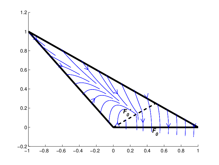
Safety constraints on both x1x_{1} and x2x_{2} determine a polyhedral state space within which the dynamics evolve. The polyhedral state space is triangulated according to Assumption 5. We focus on the reach control problem for a specific simplex of the triangulation: consider the simplex 𝒮{\mathcal{S}} determined by vertices v0=(−1,1)v_{0}=(-1,1), v1=(1,0)v_{1}=(1,0) and v2=(0,0)v_{2}=(0,0). It can be verified that 𝒪={x∈ℝ2|x2=0}{\mathcal{O}}=\{x\in{\mathbb{R}}^{2}~|~x_{2}=0\}, 𝒢=co​{v1,v2}{\mathcal{G}}=\textup{co}\{v_{1},v_{2}\}, κ=1\kappa=1, and m^=m=1\widehat{m}=m=1. Also ℬ∩cone​(𝒮)=𝟎{\mathcal{B}}\cap\textup{cone}({\mathcal{S}})={\mathbf{0}}. By the results of [7], RCP is not solvable by continuous state feedback. For example, suppose we choose control values u0=−34u_{0}=-\frac{3}{4}, u1=−1u_{1}=-1, and u2=1u_{2}=1 to satisfy the invariance conditions (2). By the method in [16], this yields an affine feedback u=[−2−3.75]​x+1u=\left[\begin{array}[]{rr}-2&-3.75\end{array}\right]x+1. Simulation of the closed-loop system is shown in Figure 8(a). We observe there exists a closed-loop equilibrium point on 𝒢{\mathcal{G}}. Now we show the problem is solvable by piecewise affine feedback.

Let b1=(0,−1)∈ℬ∩𝒞⁡(v1)b_{1}=(0,-1)\in{\mathcal{B}}\cap{\mathcal{C}}(v_{1}). Since h0=(0,−1)h_{0}=(0,-1), we have h0⋅b1>0h_{0}\cdot b_{1}>0, verifying Lemma 24. Next, we choose v′=(0.5,0.25)v^{\prime}=(0.5,0.25) along the simplex edge (v0,v1)(v_{0},v_{1}) such that from Lemma 26, h′=(−0.25,0.5)h^{\prime}=(-0.25,0.5). Then h′⋅b1<0h^{\prime}\cdot b_{1}<0 and b1∈ℬ∩cone​(𝒮1)b_{1}\in{\mathcal{B}}\cap\textup{cone}({\mathcal{S}}^{1}), verifying Lemma 27. Let 𝒮1:=co​{v′,v1,v2}{\mathcal{S}}^{1}:=\textup{co}\{v^{\prime},v_{1},v_{2}\}, 𝒮2:=co​{v0,v′,v2}{\mathcal{S}}^{2}:=\textup{co}\{v_{0},v^{\prime},v_{2}\}, and ℱ0′=co​{v′,v2}{\mathcal{F}}^{\prime}_{0}=\textup{co}\{v^{\prime},v_{2}\}. To satisfy the invariance conditions for 𝒮1{\mathcal{S}}^{1} we choose control inputs at the vertices to be u′=−1u^{\prime}=-1, u1=−1u_{1}=-1, and u12=−1u_{12}=-1. Similarly, for 𝒮2{\mathcal{S}}^{2} we choose u0=−34u_{0}=-\frac{3}{4}, u′=−1u^{\prime}=-1, and u22=1u_{22}=1. The piecewise affine feedback is

u:={[00]​x−1,x∈𝒮1[−2.0833−3.833]​x+1,x∈𝒮2.u:=\left\{\begin{array}[]{ll}\left[\begin{array}[]{rr}0&0\end{array}\right]x-1\,,&x\in{\mathcal{S}}^{1}\\ \left[\begin{array}[]{rr}-2.0833&-3.833\end{array}\right]x+1\,,&x\in{\mathcal{S}}^{2}\,.\end{array}\right.

By Theorem 6.2 of [7], 𝒮1​⟶𝒮1​ℱ0{\mathcal{S}}^{1}\overset{{\mathcal{S}}^{1}}{\longrightarrow}{\mathcal{F}}_{0} using uu. Because 𝒢2:=𝒮2∩𝒪={v2}{\mathcal{G}}^{2}:={\mathcal{S}}^{2}\cap{\mathcal{O}}=\{v_{2}\}, we have m^2=1\widehat{m}^{2}=1 and κ2=0\kappa^{2}=0 for 𝒮2{\mathcal{S}}^{2}. By Theorem 6.2 of [7], 𝒮2​⟶𝒮2​ℱ0′{\mathcal{S}}^{2}\overset{{\mathcal{S}}^{2}}{\longrightarrow}{\mathcal{F}}_{0}^{\prime} using uu. The closed-loop vector field is shown in Figure 8(b), where it is clear that RCP is solved.

Refer to caption
Refer to caption
Figure 8. Closed-loop vector fields using (a) affine feedback and (b) piecewise affine feedback.

7.2. Example 2

Consider the simplex 𝒮{\mathcal{S}} in ℝ4\mathbb{R}^{4} defined by the vertices v0=(0,0,0,0)v_{0}=(0,0,0,0), v1=(1,0,0,0)v_{1}=(1,0,0,0), v2=(0,1,0,0)v_{2}=(0,1,0,0), v3=(0,0,1,0)v_{3}=(0,0,1,0), and v4=(0,0,0,1)v_{4}=(0,0,0,1). Consider the system

x˙=[−3−3−31000−2−3−3−31000−2]​x+[0−201−2010]​u+[1111].\dot{x}=\left[\begin{array}[]{rrrr}-3&-3&-3&1\\ 0&0&0&-2\\ -3&-3&-3&1\\ 0&0&0&-2\\ \end{array}\right]x+\left[\begin{array}[]{rr}0&-2\\ 0&1\\ -2&0\\ 1&0\end{array}\right]u+\left[\begin{array}[]{r}1\\ 1\\ 1\\ 1\end{array}\right]\,.

We compute 𝒪={x∈ℝ4|x1+x2+x3+x4−1=0}{\mathcal{O}}=\{x\in{\mathbb{R}}^{4}~|~x_{1}+x_{2}+x_{3}+x_{4}-1=0\}. Thus, 𝒢=ℱ0{\mathcal{G}}={\mathcal{F}}_{0}, and we note that κ=3\kappa=3, m^=m=2\widehat{m}=m=2, and ℬ∩cone​(𝒮)=𝟎{\mathcal{B}}\cap\textup{cone}({\mathcal{S}})={\mathbf{0}}. By the results of [7], RCP is not solvable by continuous state feedback. Now we show it is solvable by piecewise affine feedback. First we examine the structure of ℬ{\mathcal{B}} (note that indices are not reordered, as is the convention in our proofs). We find by inspect that b1:=(−2,1,0,0)∈ℬ∩𝒞⁡(v1)b_{1}:=(-2,1,0,0)\in{\mathcal{B}}\cap{\mathcal{C}}(v_{1}), b3:=(0,0,−2,1)∈ℬ∩𝒞⁡(v3)b_{3}:=(0,0,-2,1)\in{\mathcal{B}}\cap{\mathcal{C}}(v_{3}), and ℬ=sp​{b1,b3}{\mathcal{B}}=\textup{sp}\{b_{1},b_{3}\}. In particular, b2:=−b1∈ℬ∩𝒞⁡(v2)b_{2}:=-b_{1}\in{\mathcal{B}}\cap{\mathcal{C}}(v_{2}) and b4:=−b3∈ℬ∩𝒞⁡(v4)b_{4}:=-b_{3}\in{\mathcal{B}}\cap{\mathcal{C}}(v_{4}). Thus, r1=2r_{1}=2 and r2=2r_{2}=2.

7.2.1. First subdivision

In the first iteration 𝒮{\mathcal{S}} is subdivided into simplices 𝒮1{\mathcal{S}}^{1} and 𝒮′{\mathcal{S}}^{\prime}. Since b2⋅h0>0b_{2}\cdot h_{0}>0, we choose v′=(0,0.75,0,0)∈(v0,v2)v^{\prime}=(0,0.75,0,0)\in(v_{0},v_{2}) such that we obtain the condition ℬ∩cone​(𝒮1)≠𝟎{\mathcal{B}}\cap\textup{cone}({\mathcal{S}}^{1})\neq{\mathbf{0}}. Hence 𝒮′{\mathcal{S}}^{\prime} = conv{v0,v1,v′,v3,v4}\{v_{0},v_{1},v^{\prime},v_{3},v_{4}\} and 𝒮1{\mathcal{S}}^{1} = conv{v′,v1,v2,v3,v4}\{v^{\prime},v_{1},v_{2},v_{3},v_{4}\}. In order to satisfy the invariance conditions for 𝒮1{\mathcal{S}}^{1} the control inputs at the vertices of 𝒮1{\mathcal{S}}^{1} are chosen as u′=(−1,−2)u^{\prime}=(-1,-2), u11=(−1,−2)u_{11}=(-1,-2), u12=(−1,−2)u_{12}=(-1,-2), u13=(−1,−2)u_{13}=(-1,-2), and u14=(1,0)u_{14}=(1,0). This yields an affine feedback

u:=[00020002]​x+[−1−2],x∈𝒮1.u:=\left[\begin{array}[]{rrrr}0&0&0&2\\ 0&0&0&2\end{array}\right]x+\left[\begin{array}[]{r}-1\\ -2\end{array}\right]\,,\qquad\qquad x\in{\mathcal{S}}^{1}\,.

For 𝒮1{\mathcal{S}}^{1} the invariance conditions are solvable and ℬ∩cone​(𝒮1)≠𝟎{\mathcal{B}}\cap\textup{cone}({\mathcal{S}}^{1})\neq{\mathbf{0}}, so by Theorem 6.2 of [7], 𝒮1​⟶𝒮1​ℱ0{\mathcal{S}}^{1}\overset{{\mathcal{S}}^{1}}{\longrightarrow}{\mathcal{F}}_{0} using uu. For 𝒮′{\mathcal{S}}^{\prime} we have 𝒢′:=𝒮′∩𝒪=co​{v1,v3,v4}{\mathcal{G}}^{\prime}:={\mathcal{S}}^{\prime}\cap{\mathcal{O}}=\textup{co}\{v_{1},v_{3},v_{4}\}. Since κ′=2\kappa^{\prime}=2 and m=2m=2, RCP is not solvable by continuous state feedback on 𝒮′{\mathcal{S}}^{\prime}, and further subdivision of 𝒮′{\mathcal{S}}^{\prime} is required.

7.2.2. Second subdivision

Consider the simplex 𝒮′=co​{v0,v1,v′,v3,v4}{\mathcal{S}}^{\prime}=\textup{co}\{v_{0},v_{1},v^{\prime},v_{3},v_{4}\}, where v′∈(v0,v2)=(0,0.75,0,0)v^{\prime}\in(v_{0},v_{2})=(0,0.75,0,0) and the exit facet is ℱ0′{\mathcal{F}}_{0}^{\prime} =conv{v1,v′,v3,v4}\{v_{1},v^{\prime},v_{3},v_{4}\}. We subdivide 𝒮′{\mathcal{S}}^{\prime} into simplices 𝒮3{\mathcal{S}}^{3} and 𝒮2{\mathcal{S}}^{2} and use a piecewise affine feedback law to solve RCP on 𝒮′{\mathcal{S}}^{\prime}. It is clear that b4⋅h0′>0b_{4}\cdot h_{0}^{\prime}>0 and therefore we can choose v′′∈(v0,v4)v^{\prime\prime}\in(v_{0},v_{4}) such that ℬ∩cone​(𝒮2)≠𝟎{\mathcal{B}}\cap\textup{cone}({\mathcal{S}}^{2})\neq{\mathbf{0}}. One choice is v′′:=(0,0,0,0.8)v^{\prime\prime}:=(0,0,0,0.8). Let 𝒮3=co​{v0,v1,v′,v3,v′′}{\mathcal{S}}^{3}=\textup{co}\{v_{0},v_{1},v^{\prime},v_{3},v^{\prime\prime}\} and 𝒮2=co​{v′′,v1,v′,v3,v4}{\mathcal{S}}^{2}=\textup{co}\{v^{\prime\prime},v_{1},v^{\prime},v_{3},v_{4}\}. It can be verified that b4∈ℬ∩cone​(𝒮2)b_{4}\in{\mathcal{B}}\cap\textup{cone}({\mathcal{S}}^{2}). To satisfy the invariance conditions for 𝒮2{\mathcal{S}}^{2} we choose u′′=(−4,0.6)u^{\prime\prime}=(-4,0.6), u21=(−5,−1)u_{21}=(-5,-1), u′=(−1,−2)u^{\prime}=(-1,-2), u23=(−5,−1)u_{23}=(-5,-1), and u24=(−3,1)u_{24}=(-3,1). To satisfy the invariance conditions for 𝒮3{\mathcal{S}}^{3} we choose u0=(0,0)u_{0}=(0,0), u31=(−1,0)u_{31}=(-1,0), u′=(−1,−2)u^{\prime}=(-1,-2), u33=(0,−1)u_{33}=(0,-1), and u′′=(−4,0.6)u^{\prime\prime}=(-4,0.6). This yields a piecewise affine feedback

u={[−1−1.330−50−2.66−10.75]​x,x∈𝒮3[39.33350−1.3302]​x+[−8−1],x∈𝒮2.u=\left\{\begin{array}[]{ll}\left[\begin{array}[]{rrrr}-1&-1.33&0&-5\\ 0&-2.66&-1&0.75\end{array}\right]x\,,&x\in{\mathcal{S}}^{3}\\ \left[\begin{array}[]{rrrr}3&9.33&3&5\\ 0&-1.33&0&2\end{array}\right]x+\left[\begin{array}[]{r}-8\\ -1\end{array}\right]\,,&x\in{\mathcal{S}}^{2}\,.\end{array}\right.

For 𝒮2{\mathcal{S}}^{2} the invariance conditions are solvable and ℬ∩cone​(𝒮2)≠𝟎{\mathcal{B}}\cap\textup{cone}({\mathcal{S}}^{2})\neq{\mathbf{0}}, so by Theorem 6.2 of [7], 𝒮2​⟶𝒮2​ℱ0′{\mathcal{S}}^{2}\overset{{\mathcal{S}}^{2}}{\longrightarrow}{\mathcal{F}}_{0}^{\prime} using uu. For 𝒮3{\mathcal{S}}^{3} we have 𝒢3=𝒮3∩𝒪=co​{v1,v3}{\mathcal{G}}_{3}={\mathcal{S}}^{3}\cap{\mathcal{O}}=\textup{co}\{v_{1},v_{3}\}. Since κ3=1\kappa^{3}=1 and m^3=2\widehat{m}^{3}=2, by Theorem 6.7 of [7], 𝒮3​⟶𝒮3​ℱ′′{\mathcal{S}}^{3}\overset{{\mathcal{S}}^{3}}{\longrightarrow}{\mathcal{F}}^{\prime\prime} using uu. Indeed, {b1,b3|bi∈ℬ∩𝒞(vi)}\{b_{1},b_{3}~|~b_{i}\in{\mathcal{B}}\cap{\mathcal{C}}(v_{i})\} is a linearly independent set associated with 𝒢3{\mathcal{G}}_{3}.

8. Conclusion

The paper studies the reach control problem on simplices, and we investigate cases when the problem is not solvable by continuous state feedback. It is shown that the class of piecewise affine feedbacks is sufficient to solve the problem in all cases of interest; namely, those cases when the problem is solvable by open-loop controls.

References

  • [1] G. Ashford and M. Broucke Reach control on simplices by time-varying affine feedback. Automatica. Accepted, December 2012. Available at: www.control.utoronto.ca/∼\simbroucke.
  • [2] C. Belta and L.C.G.J.M. Habets. Controlling a class of nonlinear systems on rectangles. IEEE Trans. Autom. Control. vol. 51, no. 11, pp. 1749–1759, Nov. 2006.
  • [3] A. Bemporad and M. Morari. Control of systems integrating logic, dynamics, and constraints. Automatica. vol. 35, pp. 407–428, March 1999.
  • [4] A. Bemporad, M. Morari, V. Dua, E. Pistikopoulos. The explicit linear quadratic regulator for constrained systems. Automatica. vol. 38, pp. 3-20, 2002.
  • [5] A. Berman and R.J. Plemmons. Nonnegative Matrices in the Mathematical Sciences. Academic Press, New York. 1979.
  • [6] K. Border. Fixed Point Theorems with Applications to Economics and Game Theory. Cambridge University Press, 1985.
  • [7] M.E. Broucke. Reach control on simplices by continuous state feedback. SIAM Journal on Control and Optimization. vol. 48, issue 5, pp. 3482-3500, February 2010.
  • [8] M.E. Broucke. On the reach control indices of affine systems on simplices. 8th IFAC Symposium on Nonlinear Control Systems. August 2010.
  • [9] M.E. Broucke and M. Ganness. Reach control on simplices by piecewise affine feedback. American Control Conference. pp. 2633-2638, June 2011.
  • [10] P. Brunovsky. A classification of linear controllable systems. Kybernetika. vol. 3, pp. 173-187, 1970.
  • [11] M.K. Camlibel, W.P.M.H. Heemels, and J.M. Schumacher. Algebraic necessary and sufficient conditions for the controllability of conewise linear systems. IEEE Trans. on Automatic Control. 53(3), pp. 762–774, 2008.
  • [12] R. Casey, H. De Jong, and J.L. Gouze. Piecewise linear models of genetic regulatory networks: Equilibria and their stability. Journal of Mathematical Biology, 52(1), pp. 27 – 56, 2006.
  • [13] F.H. Clarke, Y.S. Ledyaev, R.J. Stern, and P.R. Wolenski. Nonsmooth Analysis and Control Theory. Springer, 1998.
  • [14] R. Goebel, R.G. Sanfelice, and A.R. Teel. Hybrid Dynamical Systems. IEEE Control Systems Magazine. vol. 29, no. 2, pp. 28–93, April 2009.
  • [15] L.C.G.J.M. Habets and J.H. van Schuppen. Control of piecewise-linear hybrid systems on simplices and rectangles, in: M.D. Di Benedetto and A.L. Sangiovanni-Vincentelli (Eds.) Hybrid Systems: Computation and Control, Lecture Notes in Computer Science. Springer Verlag, vol. 2034, pp. 261–274, 2001.
  • [16] L.C.G.J.M. Habets and J.H. van Schuppen. A control problem for affine dynamical systems on a full-dimensional polytope. Automatica. no. 40, pp. 21–35, 2004.
  • [17] L.C.G.J.M. Habets, P.J. Collins, and J.H. van Schuppen. Reachability and control synthesis for piecewise-affine hybrid systems on simplices. IEEE Trans. Automatic Control. no. 51, pp. 938–948, 2006.
  • [18] C. W. Lee. Subdivisions and triangulations of polytopes. Handbook of Discrete and Computational Geometry. CRC Press Series Discrete Math. Appl., pp. 271–290, 1997.
  • [19] D. Liberzon. Switching in Systems and Control. Boston, MA: Birkhauser, 2003.
  • [20] H.H. Lin, C.L. Beck, and M.J. Bloom. On the use of multivariable piecewise linear models for predicting human response to anesthesia. IEEE Trans. on Biomedical Engineering. 51(11), pp. 1876–1887, 2004.
  • [21] Z. Lin and M.E. Broucke. On a reachability problem for affine hypersurface systems on polytopes. Automatica. vol. 47, issue 4, pp. 769-775, April 2011.
  • [22] J.R. Munkres. Elements of Algebraic Topology. Perseus Books Publishing, Cambridge, Massachusetts, 1984.
  • [23] H. Oktem. A survey on piecewise linear models of regulatory dynamical systems. Nonlinear Analysis: Theory Methods and Applications. 63(3), pp. 336–349, 2005.
  • [24] R.J. Ramadge and W.M. Wonham. Supervisory control of a class of discrete event processes. SIAM J. Control and Optimization. vol. 25, no. 1, pp. 206-230, 1987.
  • [25] R.T Rockafellar. Convex Analysis. Princeton University Press, Princeton, New Jersey 1970.
  • [26] B. Roszak and M. E. Broucke. Necessary and sufficient conditions for reachability on a simplex. Automatica. vol. 42, no. 11, pp. 1913–1918, November 2006.
  • [27] B. de Schutter and T.J.J. van den Boom. MPC for continuous piecewise-affine systems. Systems and Control Letters. 52(3-4), pp. 179–192, 2004.
  • [28] F. Tahami and B. Molaei. Piecewise affine system modeling and control of PWM converters. Journal of Circuits Systems and Computers, 16(1), pp. 113 – 128, 2007.
  • [29] W.M. Wonham. Linear Multivariable Control: a Geometric Approach. 3rd Edition, Springer, 1985.

9. Appendix

Proof of Theorem 7.

Let x0∈𝒮∖ℱ0x_{0}\in{\mathcal{S}}\setminus{\mathcal{F}}_{0}. By assumption there exists μx0​(t)\mu_{x_{0}}(t) and a time T⁡(x0)>0T(x_{0})>0 such that ϕμx0​(t,x0)∈𝒮\phi_{\mu_{x_{0}}}(t,x_{0})\in{\mathcal{S}} for all t∈[0,T⁡(x0)]t\in[0,T(x_{0})]. Since μx0​(t)\mu_{x_{0}}(t) is an open-loop control, there exists c≥0c\geq 0 such that ‖μx0​(t)‖≤c\|\mu_{x_{0}}(t)\|\leq c, for all t∈[0,T⁡(x0)]t\in[0,T(x_{0})]. Define 𝒴⁡(x):={A​x+B​w+a|w∈ℝm}{\mathcal{Y}}(x):=\bigl\{Ax+Bw+a~|~w\in{\mathbb{R}}^{m}\bigr\} and 𝒴c(x):={Ax+Bw+a|w∈ℝm,∥w∥≤c}{\mathcal{Y}}_{c}(x):=\bigl\{Ax+Bw+a~|~w\in{\mathbb{R}}^{m},\|w\|\leq c\bigr\}. Now take a sequence {ti|ti∈(0,T⁡(x0)]}\{t_{i}~|~t_{i}\in(0,T(x_{0})]\} with ti→0t_{i}\rightarrow 0. Since {y∈𝒴c​(x)|x∈𝒮}\{y\in{\mathcal{Y}}_{c}(x)~|~x\in{\mathcal{S}}\} is bounded, there exists M>0M>0 such that ‖ϕμx0​(ti,x0)−x0‖≤M​ti\|\phi_{\mu_{x_{0}}}(t_{i},x_{0})-x_{0}\|\leq Mt_{i}. Therefore {ϕμx0​(ti,x0)−x0ti}\{\frac{\phi_{\mu_{x_{0}}}(t_{i},x_{0})-x_{0}}{t_{i}}\} is a bounded sequence, and there exists a convergence subsequence (with indices relabeled) such that limi→∞ϕμx0​(ti,x0)−x0ti=:v\lim_{i\rightarrow\infty}\frac{\phi_{\mu_{x_{0}}}(t_{i},x_{0})-x_{0}}{t_{i}}=:v. Since ϕμx0​(ti,x0)∈𝒮\phi_{\mu_{x_{0}}}(t_{i},x_{0})\in{\mathcal{S}}, by the definition of the Bouligand tangent cone, v∈T𝒮​(x0)v\in T_{{\mathcal{S}}}(x_{0}). On the other hand, we have

ϕμx0​(ti,x0)−x0ti=1ti​∫0ti[A​ϕμx0​(τ,x0)+B​μx0​(τ)+a]​𝑑τ.\frac{\phi_{\mu_{x_{0}}}(t_{i},x_{0})-x_{0}}{t_{i}}=\frac{1}{t_{i}}\int_{0}^{t_{i}}\bigl[A\phi_{\mu_{x_{0}}}(\tau,x_{0})+B{\mu_{x_{0}}}(\tau)+a\bigr]d\tau\,. (22)

Taking the limit, we get

v=A​x0+B​limi→∞μx0​(ti)+a∈𝒴⁡(x0).v=Ax_{0}+B\lim_{i\rightarrow\infty}{\mu_{x_{0}}}(t_{i})+a\in{\mathcal{Y}}(x_{0})\,.

We conclude that 𝒴⁡(x0)∩T𝒮​(x0)≠∅{\mathcal{Y}}(x_{0})\cap T_{{\mathcal{S}}}(x_{0})\neq\emptyset, x0∈𝒮∖ℱ0x_{0}\in{\mathcal{S}}\setminus{\mathcal{F}}_{0}. Since T𝒮​(v0)=cone​(𝒮)T_{{\mathcal{S}}}(v_{0})=\textup{cone}({\mathcal{S}}), and T𝒮​(x)=𝒞⁡(vi)T_{{\mathcal{S}}}(x)={\mathcal{C}}(v_{i}) for x∈(v0,vi)x\in(v_{0},v_{i}), it follows that the invariance conditions are solvable at v0v_{0} and along simplex edges (v0,vi),i∈I(v_{0},v_{i}),i\in I.

Now consider vi,i∈Iv_{i},i\in I. If vi∈𝒪v_{i}\in{\mathcal{O}}, then the invariance conditions are solvable by selecting ui∈ℝmu_{i}\in{\mathbb{R}}^{m} such that A​vi+B​ui+a=0Av_{i}+Bu_{i}+a=0. Instead suppose vi∉𝒪v_{i}\not\in{\mathcal{O}}. Suppose by way of contradiction that 𝒴⁡(vi)∩𝒞⁡(vi)=∅{\mathcal{Y}}(v_{i})\cap{\mathcal{C}}(v_{i})=\emptyset. Then 𝒴⁡(vi){\mathcal{Y}}(v_{i}) and 𝒞⁡(vi){\mathcal{C}}(v_{i}) are non-empty disjoint polyhedral convex sets in ℝn{\mathbb{R}}^{n}. By Corollary 19.3.3 of [25], they are strongly separated. That is, there exists ϵ>0\epsilon>0 such that infy∈𝒴⁡(vi),z∈𝒞⁡(vi)‖y−z‖>ϵ\inf_{y\in{\mathcal{Y}}(v_{i}),z\in{\mathcal{C}}(v_{i})}\|y-z\|>\epsilon. By the upper semicontinuity of x↦𝒴⁡(x)x\mapsto{\mathcal{Y}}(x), there exists δ>0\delta>0 such that if ‖x−vi‖<δ\|x-v_{i}\|<\delta, then 𝒴⁡(x)⊂𝒴⁡(vi)+ϵ2​ℬ{\mathcal{Y}}(x)\subset{\mathcal{Y}}(v_{i})+\frac{\epsilon}{2}{\mathscr{B}}. In particular, taking x∈(v0,vi)x\in(v_{0},v_{i}), we get 𝒴⁡(x)∩𝒞⁡(vi)=∅{\mathcal{Y}}(x)\cap{\mathcal{C}}(v_{i})=\emptyset, a contradiction. ∎

Proof of Theorem 8.

Consider vi∈V∩𝒢v_{i}\in V\cap{\mathcal{G}}. Suppose ℬ∩𝒞⁡(vi)=𝟎{\mathcal{B}}\cap{\mathcal{C}}(v_{i})={\mathbf{0}}. Since A​vi+a∈ℬAv_{i}+a\in{\mathcal{B}}, there exists ui∈ℝmu_{i}\in{\mathbb{R}}^{m} such that A​vi+B​ui+a=0Av_{i}+Bu_{i}+a=0. By (ii)-(iii) of Definition 6, there exists ε>0\varepsilon>0 such that for all x∈𝒮∖ℱ0x\in{\mathcal{S}}\setminus{\mathcal{F}}_{0}, there exists ux∈ℝmu_{x}\in{\mathbb{R}}^{m} such that A​x+B​ux+a∈T𝒮​(x)Ax+Bu_{x}+a\in T_{{\mathcal{S}}}(x) and ‖A​x+B​ux+a‖>ε\|Ax+Bu_{x}+a\|>\varepsilon. By continuity there exists δ>0\delta>0 such that if ‖x−vi‖<δ\|x-v_{i}\|<\delta, then ‖A​x+B​ui+a‖<ε/2\|Ax+Bu_{i}+a\|<\varepsilon/2. Thus, for x∈𝒮∖ℱ0x\in{\mathcal{S}}\setminus{\mathcal{F}}_{0} with ‖x−vi‖<δ\|x-v_{i}\|<\delta, we have ‖B⁡(ux−ui)‖>ε/2\|B(u_{x}-u_{i})\|>\varepsilon/2. Since ℬ∩𝒞⁡(vi)=𝟎{\mathcal{B}}\cap{\mathcal{C}}(v_{i})={\mathbf{0}} and 𝒞⁡(vi){\mathcal{C}}(v_{i}) is a closed cone, there exists α>0\alpha>0 such that if b∈ℬb\in{\mathcal{B}} satisfies ‖b‖>ε/2\|b\|>\varepsilon/2, then (b+α​ℬ)∩𝒞⁡(vi)=∅(b+\alpha{\mathscr{B}})\cap{\mathcal{C}}(v_{i})=\emptyset. In particular, we can choose x∈(v0,vi)x\in(v_{0},v_{i}) sufficiently close to viv_{i} such that ‖A​x+B​ui+a‖<min⁡{α,ϵ/2}\|Ax+Bu_{i}+a\|<\min\{\alpha,\epsilon/2\}. Then A​x+B​ux+a=(A​x+B​ui+a)+B⁡(ux−ui)∉𝒞⁡(vi)=T𝒮​(x)Ax+Bu_{x}+a=(Ax+Bu_{i}+a)+B(u_{x}-u_{i})\not\in{\mathcal{C}}(v_{i})=T_{{\mathcal{S}}}(x), a contradiction. ∎