Joint Sensing and Power Allocation
in Nonconvex Cognitive Radio Games: Nash Equilibria and Distributed
AlgorithmsThanks: The work of Pang is based on research supported by the U.S.A. National
Science Foundation grant CMMI 0969600 and by the Air Force Office
of Sponsored Research award No. FA9550-09-10329. The work of Scutari
was supported by U.S.A. National Science Foundation grant CSM 1218717.
Copyright (c) 2012 IEEE. Personal use of this material is permitted.
However, permission to use this material for any other purposes must
be obtained from the IEEE by sending a request to pubs-permissions@ieee.org.
Abstract
In this paper, we propose a novel class of Nash problems for Cognitive Radio (CR) networks, modeled as Gaussian frequency-selective interference channels, wherein each secondary user (SU) competes against the others to maximize his own opportunistic throughput by choosing jointly the sensing duration, the detection thresholds, and the vector power allocation. The proposed general formulation allows to accommodate several (transmit) power and (deterministic/probabilistic) interference constraints, such as constraints on the maximum individual and/or aggregate (probabilistic) interference tolerable at the primary receivers. To keep the optimization as decentralized as possible, global (coupling) interference constraints are imposed by penalizing each SU with a set of time-varying prices based upon his contribution to the total interference; the prices are thus additional variable to optimize. The resulting players’ optimization problems are nonconvex; moreover, there are possibly price clearing conditions associated with the global constraints to be satisfied by the solution. All this makes the analysis of the proposed games a challenging task; none of classical results in the game theory literature can be successfully applied.
The main contribution of this paper is to develop a novel optimization-based theory for studying the proposed nonconvex games; we provide a comprehensive analysis of the existence and uniqueness of a standard Nash equilibrium, devise alternative best-response based algorithms, and establish their convergence. Some of the proposed algorithms are totally distributed and asynchronous, whereas some others require limited signaling among the SUs (in the form of consensus algorithms) in favor of better performance; overall, they are thus applicable to a variety of CR scenarios, either cooperative or noncooperative, which allows the SUs to explore the existing trade-off between signaling and performance.
1 Introduction
Over the past decade, there has been a growing interest in Cognitive Radio (CR) as an emerging paradigm to address the de jure shortage of allocated spectrum that contrasts with the de facto abundance of unused spectrum in virtually any spatial location at almost any given time. The paradigm posits that so-called cognitive radios [also termed as secondary users (SUs)] would use licensed spectrum in an ad-hoc fashion in such a way as to cause no harmful interference to the primary spectrum license holders [also termed as primary users (PUs)]. Evidently, such an opportunistic spectrum access is intertwined with the design of multiple secondary system components, such as (but not limited to) spectrum sensing and transmission parameters adaptation. Indeed, the choice of the sensing parameters (e.g., the detection thresholds and the sensing duration) as well as the consequent design of the physical layer transmission strategies (e.g., the transmission rate, the power allocation) have both a direct impact on the performance of primary and secondary systems. The interplay between these two interacting components calls for a joint optimization of the sensing and transmission parameters of the SUs, which is the main focus of this paper.
1.1 Motivation and related work
The joint optimization of the sensing and transmission strategies has been only partially addressed in the literature, even for simple CR scenarios composed of one PU and one SU. For example, in [1, 2], the authors proposed alternative centralized schemes that optimize the detection thresholds for a bank of energy detectors, in order to maximize the opportunistic throughput of a SU, for a given sensing time and constant-rate/power transmissions. The optimization of the sensing time and the sensing time/detection thresholds for a given missed detection probability and constant rate of one SU was addressed in [3, 4] and [5], respectively. A throughput-sensing trade-off for a fixed transmission rate was studied in [6]. In [7] (or [8]) the authors focused on the joint optimization of the power allocation and the equi-false alarm rate (or the sensing time) of a SU over multi-channel links, for a fixed sensing time (or detection probability). All the aforementioned schemes however are not applicable to scenarios composed of multiple SUs (and PUs). The case of multiple SUs and one PU was considered in [9] (and more recently in [10]), under the same assumptions of [7]; however no formal analysis of the proposed formulation was provided.
The transceiver design of OFDM-based CR systems composed of multiple primary and secondary users have been largely studied in the literature of power control problems over the interference channel, and have been traditionally approached from two very different perspectives: a holistic design of the system and an individual selfish design of each of the users. The former is also referred to as Network Utility Maximization (NUM) (other approaches within this perspective are based on Nash bargaining formulations) and has the potential of obtaining the best of the network at the expense of a centralized computation or heavy signaling/cooperation among the users; examples are [11, 12, 13, 14, 15, 16, 17]. The latter fits perfectly within the mathematical framework of Game Theory and usually leads to distributed algorithms at the expense of a loss of global performance; related papers are [18, 19, 20, 21, 22, 23], and two recent overviews are [24, 25]. In both the aforementioned approaches and classes of papers the sensing process is not considered as part of the optimization; in fact the SUs do not perform any sensing but they are allowed to transmit over the licensed spectrum provided that they satisfy interference constraints imposed by the PUs, no matter if the PUs are active of not.
When the sensing comes explicitly into the system design, the application of the holistic approach mentioned above leads to nonconvex NP hard optimization problems. These cases cannot be globally solved by efficient algorithms in polynomial time; one typically can design (centralized) sub-optimal algorithms that converge just to a stationary solution. Their implementation however would require heavy signaling among the users (or the presence of a centralized network controller having the knowledge of all the system parameters); which strongly limits the range of applicability of such formulations to practical CR networks. For these reasons, in this paper, we attack the multi-agent decision making problem from a different perspective; we concentrate on optimization strategies where the SUs are able to self-enforce the negotiated agreements on the usage of the licensed spectrum either in a totally decentralized way or by requiring limited and local signaling among the SUs (in the form of consensus algorithms). Aiming at exploring the trade-off between signaling and performance, the proposed approach is then expected to be more flexible than classical optimization techniques and applicable to a wider range of CR scenarios.
1.2 Main contributions
This paper along with our companion work [26] advances the current approaches (based on the optimization of specific components of a CR system in isolation), in the direction of a joint and distributed design of sensing and transmission parameters of a CR network, composed of multiple PUs and SUs.
We study a novel class of Nash equilibrium problems as proposed in [26], wherein each SU aims at maximizing his own opportunistic throughput by jointly optimizing the sensing parametersthe sensing time and the false alarm rate (and thus the decision thresholds) of a bank of energy detectorsand the power allocation over the multi-channel links. Because of sensing errors, the SUs might access the licensed spectrum when it is still occupied by active PUs, thus causing harmful interference. This motivates the introduction of probabilistic interference constraints that are imposed to control the power radiated over the licensed spectrum whenever a missed detection event occurs (in a probabilistic sense). The proposed formulation accommodates alternative combinations of power/interference constraints. For instance, on top of classical (deterministic) transmit power (and possibly spectral masks) constraints, we envisage the use of average individual (i.e., on each SU) and/or global (i.e., over all the SUs) interference tolerable at the primary receivers. The former class of constraints is more suitable for scenarios where the SUs are not willing to cooperate; whereas the latter constraints, which are less conservative, seem more realistic in settings where SUs may want to trade some limited signaling for better performance. By imposing a coupling among the transmit and sensing strategies of the SUs, global interference constraints introduce a new challenge in the system design: how to enforce global interference constraints without requiring a centralized optimization but possibly only limited signaling among the SUs? We address this issue by introducing a pricing mechanism in the game, through a penalization in the players’ objective functions. The prices need to be chosen so that the interference constraints are satisfied at any solution of the game and a clearing condition holds; they are thus additional variables to be determined.
The resulting class of games is nonconvex (because of the nonconvexity of the players’ payoff functions and constraints), lacks boundedness in the price variables, and there are side constraints with associated price equilibration that are required to be satisfied by the equilibrium; all these features make the analysis a challenging task. The convexity of the players’ individual optimization problems is, in fact, one indispensable assumption under which noncooperative games have traditionally been studied and analyzed. The classical case where a NE exists is indeed when the players’ objective functions are (quasi-)convex in their own variables with the other players’ strategies fixed, and the players’ constraint sets are compact and convex and independent of their rivals’ strategies (see, e.g., [27, 28]). Without such convexity, a NE may not exist (as in the well-known case of a matrix game with pure strategies); analytically, abstract mathematical theories granting its existence, like those in [29, 30], are difficult to be applied to games arising from realistic applications such as those occurred in the present paper.
The main contribution of this work is to develop a novel optimization-based theory for the solution analysis of the proposed class of nonconvex games (possibly) with side constraints and price clearing conditions, and to design distributed best-response based algorithms for computing the Nash equilibria, along with their convergence properties. Building on [31], the solution analysis is addressed by introducing a “best-response” map (including price variables) defined on a proper convex and compact set, whose fixed-points, if they exist, are Nash equilibria of the original nonconvex games; the obtained conditions are in fact sufficient for such a map to be a single-valued continuous map; this enables the application of the Brouwer fixed-point theorem to deduce the existence of a fixed-point of the best-response map, thus of a NE of the whole class of proposed games. While seemingly very simple, the technical details lie in deriving (reasonable) conditions for which the best-response map is single-valued and for the boundedness of the prices in order for the existence of a compact set on which the Brouwer result can be based. Interestingly, the obtained conditions have the same physical interpretation of those obtained for the convergence of the renowned iterative waterfilling algorithm solving the power control game over interference channels [18, 19, 20, 21, 22]. We then focus on solutions schemes for the proposed class of games; we design alternative distributed (possibly) asynchronous best-response based algorithms that differ in performance, level of protection of the PUs, computational effort and degree of cooperation/signaling among the SUs, and convergence speed; which makes them applicable to a variety of CR scenarios (either cooperative or noncooperative). For each algorithm, we establish its convergence and also quantify the time and communication costs for its implementation. Our numerical results show that: i) the proposed joint sensing/transmission optimization outperforms current centralized and decentralized state-of-the-art results based on separated optimization of the sensing and the transmission parts; ii) our algorithms exhibit a fast convergence behavior; and iii) as expected, some (limited) cooperation among the SUs (in the form of consensus algorithms) yields a significant improvement in the system performance. The proposed solution schemes can also be used to compute the so-called Quasi-NE of the associated games, a relaxed equilibrium concept introduced and studied in our companion paper [26].
The paper is organized as follows. Sec. 2 briefly introduces the system model, as proposed in [26]; Sec. 3 focuses on the system design and formulates the joint optimization of the sensing parameters and the power allocation of the SUs within the framework of game theory; several games are introduced. The solution analysis of the proposed games is addressed in Sec. 4, where sufficient conditions for the existence and uniqueness of a standard NE along with their interpretation are derived. Distributed algorithms solving the proposed games along with their convergence properties and computational/communication complexity are studied in Sec. 5. Numerical experiments are reported in Sec. 6, whereas Sec. 7 draws the conclusions. Proofs of our results are given in Appendix A-F. The paper requires a background on Variational Inequalities (VIs); we refer to [32, 33] for an introductory overview of the subject and its application to equilibrium problems in signal processing and communications. A comprehensive treatment of VIs can be found in the two monographs [34, 35]; a detailed study of convex games based on the VI and complementarity approach is addressed in [36, 22]. The main properties of Z and P matrices, which are widely used in the paper, can be found in [34, 37].
2 System Model
We consider a scenario composed of active SUs, each consisting of a transmitter-receiver pair, coexisting in the same area and sharing the same band with PUs. The network of the SUs is modeled as an -frequency-selective SISO Interference Channel (IC), where is the number of subcarriers available to the cognitive users. We focus on multicarrier block-transmissions without loss of generality. In order not to interfere with on-going PU transmissions, before transmitting, the SUs sense periodically the licensed spectrum looking for the subcarriers that are temporarily not occupied by the PUs. A brief description of the sensing mechanism and transmission phase performed by the SUs as proposed in the companion paper [26] is given in the following, where we introduce the basic definitions and notation used throughout the paper; we refer the reader to [26] for details and the assumptions underlying the proposed model.
2.1 The spectrum sensing phase
In [26], we formulated the sensing problem as a binary hypothesis testing; the decision rule of SU over carrier based on the energy detector is
| (1) |
where is the received baseband complex signal over carrier ; is the number of samples, with and denoting the sensing time and the sampling frequency, respectively; is the decision threshold for the carrier ; represents the absence of any primary signal over the subcarrier , whereas represents the presence of the primary signaling.
The performance of the energy detection performed by SU over carrier is measured in terms of the detection probability and false alarm probability . Under standard assumptions in decision theory, these probabilities are given by [26]
| (2) |
where is the Q-function, and , , , and are constant parameters, whose explicit expressions are given in [26]. The detection probability can also be rewritten as a function of the false alarm rate as:
| (3) |
where we also introduced the definition of the missed detection probability .
The interpretation of and within the CR scenario is the following: signifies the probability of successfully identifying from the SU a spectral hole over carrier , whereas the missed detection probability represents the probability of SU failing to detect the presence of the PUs on the subchannel and thus generating interference against the PUs. The free variables to optimize are the detection thresholds ’s and the sensing times ’s; ideally, we would like to choose ’s and ’s in order to minimize both and , but (3) shows that there exists a trade-off between these two quantities that will affect both primary and secondary performance. It turns out that, ’s and ’s can not be chosen by focusing only on the detection problem (as in classical decision theory), but the optimal choice of and must be the result of a joint optimization of the sensing and transmission strategies over the two phases; such an optimization is introduced in Sec. 3.
Robust sensing model. The proposed sensing model can be generalized in several directions; see [38, 26]. For instance, one can explicitly take into account device-level uncertainties (e.g., uncertainty in the power spectral density of the PUs’ signals and thermal noise) as well as system level uncertainties (e.g., the current number of active PUs) by modeling the detection process of the primary signals as a composite hypothesis testing. This leads to a uniformly most-powerful detector scheme that is robust against device-level and system-level uncertainties; detailed can be found in [38, 26] and are omitted here. It is important however to remark that the resulting detection probability and false alarm rate of the aforementioned robust scheme are still given by (2) and (3), but with a different expression for ’s and ’s [38]. This means that analysis and results developed in the next sections are valid also for this more general model.
2.2 The transmission phase
The transmission strategy of each SU is the power allocation vector over the subcarriers, subject to the following (local) transmit power constraints
| (4) |
where denotes possibly spectral mask [the vector inequality in (4) is component-wise].
According to the opportunistic transmission paradigm, each subcarrier is available for the transmission of SU if no primary signal is detected over that frequency band, which happens with probability . This motivates the use of the aggregate opportunistic throughput as a measure of the spectrum efficiency of each SU . Given the power allocation profile of the SUs, the target false alarm rate (assumed to be equal over the whole licensed spectrum), the sensing time , and taking the log of the opportunistic throughput, the payoff function of each SU is then (see [26] for more details)
| (5) |
where , with , is the portion of the frame duration available for opportunistic transmissions and is the maximum information rate achievable on link over carrier when no primary signal is detected and the power allocation profile of the SUs is :
| (6) |
with and , where is the channel transfer function of the direct link and is the cross-channel transfer function between the secondary transmitter and the secondary receiver ; and is the power spectral density (PSD) of the background noise over carrier at the receiver (assumed to be Gaussian zero-mean distributed).
As a final remark note that the throughput defined in (5) is not the average throughput experienced by the SUs, which instead would include an additional rate contribution resulting from the erroneous decision of the SUs to transmit over the licensed spectrum still occupied by the PUs. We have not included this contribution in the objective functions of the SUs because in maximizing the function we do not want to “incentivize” the undue usage of the licensed spectrum. Moreover, differently from the opportunistic throughput in (5), the maximization of the average throughput would require the knowledge from the SUs of the a-priori probabilities of the PUs’ spectrum occupancy, which is in general not available.
2.3 Probabilistic interference constraints
Due to the inherent trade-off between and [see (2) and (3)], maximizing the aggregate opportunistic throughput (5) of SUs will result in low and thus large , hence causing harmful interference to PUs. To allow the SUs’ transmissions while preserving the QoS of the PUs, we envisage the use of probabilistic interference constraints that limit the interference generated by the SUs whenever they misdetect the presence of a PU. Examples of these constraints are the following:
- -
-
Individual overall bandwidth interference constraint: for each SU
(7) - -
-
Global overall bandwidth interference constraints:
(8)
where [or ] are the maximum average interference allowed to be generated by the SU [or all the SU’s] that is tolerable at the primary receiver; and ’s are a given set of positive weights. If an estimate of the cross-channel transfer functions between the secondary transmitters and the primary receiver is available, then the natural choice for is , so that (7) and (8) become the average interference experienced at the primary receiver. Methods to obtain the interference limits along with some implementation aspects related to this issue and alternative interference constraints are discussed in Sec. 5.1.1.
We wish to point out that other interference constraints, like per-carrier interference constraints, as well as multiple PUs can be readily accommodated, without affecting the analysis and results that will be presented in the forthcoming sections. For notational simplicity, we stay within the above setting.
3 System Design based on Game Theory
We focus now on the system design and formulate the joint optimization of the sensing parameters and the power allocation of the SUs within the framework of game theory. We consider next two classes of equilibrium problems: i) games with individual constraints only (Sec. 3.1 below); and ii) games with individual and global constraints (Sec. 3.1 and Sec. 3.3 below). The former formulation is suitable for modeling scenarios where the SUs are selfish users who are not willing to cooperate, whereas the latter class of games is applicable to the design of systems where the SUs can exchange limited signaling in favor of better performance. Indeed, being less conservative than individual interference constraints, global interference constraints are expected to yield better performance of the SUs at the cost of more signaling. The aforementioned formulations are thus applicable to complementary CR scenarios.
3.1 Game with local interference constraints
In the proposed game, each SU is modeled as a player who aims to maximize his own opportunistic throughput by choosing jointly a proper power allocation strategy , sensing time , and false alarm rate , subject to power and individual probabilistic interference constraints. Stated in mathematical terms we have the following formulation.
Player ’s optimization problem is to determine, for given , a tuple in order to (9)
In (9) we also included additional lower and upper bounds of satisfying and upper bounds on detection and missed detection probabilities and , respectively. These bounds provide additional degrees of freedom to limit the probability of interference to the PUs as well as to maintain a certain level of opportunistic spectrum utilization from the SUs []. Note that the constraints and do not represent a real loss of generality, because practical CR systems are required to satisfy even stronger constraints on false alarm and detection probabilities; for instance, in the WRAN standard, .
3.2 Game with global interference constraints
We add now global interference constraints to the game theoretical formulation in (9). This introduces a new challenge: how to enforce global interference constraints in a distributed way? By imposing a coupling among the transmissions and the sensing strategies of all the SUs, global interference constraints in principle would call for a centralized optimization. To overcome this issue, we introduce a pricing mechanism in the game, based on the relaxation of the coupling interference constraints as penalty term in the SUs’ objective functions, so that the interference generated by all the SUs will depend on these prices. Prices are thus addition variables to be optimized (there is one common price associated with any of the global interference constraints); they must be chosen so that any solution of the game will satisfy the global interference constraints, which requires the introduction of additional constraints on the prices, in the form of price clearance conditions. Denoting by the price variable associated with the global interference constraint (8), we have the following formulation.
Player ’s optimization problem is to determine, for given and , a tuple such that (10) Price equilibrium: The price obeys the following complementarity condition: (11)
In (11), the compact notation means , , and . The price clearance conditions (11) state that global interference constraints (8) must be satisfied together with nonnegative price; in addition, they imply that if the global interference constraint holds with strict inequality then the price should be zero (no penalty is needed). Thus, at any solution of the game, the optimal price is such that the global interference constraint is satisfied.
3.3 The equi-sensing case
The decision model proposed in Sec. 2.1 is based on the assumption that the SUs are somehow able to distinguish between primary and secondary signaling. This can be naturally accomplished if there is a common sensing time (still to optimize) during which all the SUs stay silent while sensing the spectrum. However, the formulation (10), in general, leads to different optimal sensing times of the SUs, implying that some SU may start transmitting while some others are still in the sensing phase. To overcome this issue, several directions have been explored in the companion paper [26], under the model (10)-(11). Here we follow the approach of modifying the formulation in (10) in order to “force” in a distributed way the same optimal sensing time for all the SUs. Roughly speaking, the idea is to perturb the payoff functions of the players by a penalty term that discourages the players to deviate from equi-sensing strategies. Stated in mathematical terms, we have the following formulation.
Player ’s optimization problem is to determine, for given , and , a tuple in order to (12) Price equilibrium: The price obeys the complementarity condition (11).
The third term in the objective function of each SU in (12) helps to induce the same optimal sensing time for all the SUs. Roughly speaking, one expects that for sufficiently large , the aforementioned term will become the dominant term in the objective functions of the SUs, leading thus to solutions of the game having sensing times that differ from their average by any prescribed accuracy. This intuition has been made formal in our companion paper [26] for stationary solutions of the game (12), and it can be similarly extended to the Nash equilibria; we omit the details because of space limitation.
3.4 Unified formulation and summary of notation
In this section, we introduce a compact and unified formulation of the proposed games that simplifies their analysis. Let us start by separating the convex constraints in the feasible set of the players from the nonconvex ones. The interference constraints (a) in (9) are bi-convex and thus not convex, whereas constraints (b) are convex in and . This motivates the following change of variables:
| (13) |
so that the constraints on in each player’s feasible set become convex in the tuple [with ]. Indeed, for each , we have
| (14) |
where denotes the inverse of the Q-function [ is a strictly decreasing function on ], which are convex constraints in [provided that ]. Using the above transformation, we can equivalently rewrite the missed detection probability and the throughput of each player in terms of the tuples ’s, denoted by and , respectively; the explicit expression of these quantities is:
| (15) |
| (16) |
To incorporate the equi-sensing case in our unified formulation, we introduce the functions , which represent the objective functions of the users including the equi-sensing term, with denoting the strategy profile of all the players:
| (17) |
We can now rewrite the feasible set of each player’s optimization problem in terms of the new variables , denoted by : for each let
| (18) |
where we have separated the convex part and the nonconvex part; the convex part is given by the polyhedron corresponding to the constraints (b) and (c) in (9) under the transformation (13) [cf. (14)]:
| (19) |
with
| (20) |
whereas the nonconvex part in (18) is given by the constraint (a) that we have rewritten as by introducing the local interference violation function
| (21) |
This measures the violation of the local interference constraint (a) at . Similarly, it is convenient to introduce also the global interference violation function , which depends on the strategy profile of all the players:
| (22) |
measures the violation of the global interference constraint (8) at ; global interference constraints (8) can be then rewritten in terms of as .
Based on the above definitions, throughout the paper, we will use the following notation. The convex part of the joint strategy set is denoted by , whereas the set containing all the (convex part of) players’ strategy sets except the -th one is denoted by ; similarly, we define and . For notational simplicity, when it is needed, we will use interchangeably either or to denote the strategy tuple of player ; similarly, the strategy profile of all the players will be denoted either by or , with , and , whereas is the strategy profile of all the players except the -th one. All the tuples above are intended to be column vectors; for instance, signifies , with , where each and For future convenience, Table 1 collects the above definitions and symbols. Using the above notation, the games introduced in the previous sections can be unified under the following reformulation.
Players’ optimization. The optimization problem of player is: (23) Price equilibrium. The price obeys the following complementarity condition: (24)
Throughout the paper, we will refer to the game (23) along with the side constraint (24) as game , where .
| Symbol | Meaning |
|---|---|
| sensing time of SU | |
| power allocation vector of SU | |
| scalar price variable | |
| false alarm probability of SU | |
| missed detection probability of SU on carrier [cf. (3)] | |
| normalized sensing time of SU [cf. (13)] | |
| strategy tuple of SU | |
| strategy profile of all the SUs except the -th one | |
| strategy profile of all the SUs | |
| payoff function of SU including the equisensing penalization [cf. (17)] | |
| local interference constraint violation of SU [cf. (21)] | |
| global interference constraint violation of SU [cf. (22)] | |
| , | feasible set of SU [cf. (18)], joint feasible strategy set of |
| joint strategy set of the SUs except the -th one | |
| , | convex part of [cf. (19)], Cartesian product of all ’s |
Needless to say, when and , reduces to the game in (9) where there are only individual interference constraints (7), whereas when , coincides with the game in (10)-(11) with local and global interference constraints.
As a final remark, we observe that the proposed formulations may be extended to cover more general settings, without affecting the validity of the results we are going to present. For instance, the case of multiple active PUs and additional local/global interference constraints (such as per-carrier constraints) can be readily accommodated: Instead of having a single price variable, we associate a different price to each global interference constraint and proceed similarly as in (23)-(24). Also, the sensing model introduced in Sec. 2.1 can be generalized to the case of multiple active PUs, and the presence of device-level uncertainties (e.g., uncertainty in the power spectral density of the PUs’ signals and thermal noise) as well as system level uncertainties (e.g., lack of knowledge of the number of active PUs). The mathematical details of these more general formulations can be found in our companion paper [26]; for notational simplicity, here we will stay within the formulation (23)-(24), without loss of generality.
4 Solution Analysis: Nash Equilibria
This section is devoted to the solution analysis of the games introduced in the previous section. In order to provide a unified analysis, we focus on the general game with side constraints; results for the other proposed formulations are obtained as special cases. We start our analysis by studying the feasibility of each optimization problem in (23) (cf. Sec. 4.1); we then extend the definitions of NE to a game with side constraints and establish its main properties (cf. Sec. 4.2).
4.1 Feasibility conditions
Introducing the SNR detection experimented by SU over carrier and using the definitions given in Sec. 2.1, sufficient conditions guaranteeing the existence of an optimal solution for each player’s optimization problem (23) are the following: For all and , there must exist a common sensing time (corresponding to normalized sensing times ) such that
| (25) |
The first set of conditions in (25) simply postulates the existence of an overlap among the (normalized) sensing time intervals in (23), which is necessary to guarantee the existence of a common value for the sensing times in the original variables ’s. The second set of conditions guarantees that the strategy sets ’s (and thus ’s) are not empty. Interestingly, they quantify the existing trade-off between the sensing time (the product “time-bandwidth” of the system) and detection accuracy: the smaller both false alarm and missed detection probability values, the larger the sensing time (the decision process must be more accurate).
When the sensing times are not forced to be the same, as in the formulations (9) and (10)-(11), the feasibility conditions (25) can be weakened by the following: For all and ,
| (26) |
Throughout the paper, we tacitly assume that each user’s optimization problem under consideration has a nonempty strategy set (the associated feasibility conditions above are satisfied).
4.2 Existence and uniqueness of the NE
We focus in this section on the NE of . The definition of NE for a game with price equilibrium conditions such as is the natural generalization of the same concept introduced for classical noncooperative games having no side constraints (see, e.g., [27]) and is given next.
Definition. A Nash equilibrium of the game is a strategy-price tuple , such that (27) and (28) A NE is said to be trivial if the power-component for all .
In words, the proposed notion of equilibrium is a stable state of the network consisting of an equilibrium power/sensing profile and price : at , the SUs have no incentive to change their power/sensing profiles based on the current state of the network [represented by (27)], while the optimal value of the price is such that all global interference constraints are met [a situation represented by (28)]. Note that, for a set of fixed price , the equilibrium power/sensing profile can be interpreted as the NE of a classical noncooperative game (having thus only local constraints), wherein the payoff function of each player is and the strategy set is . The proposed equilibrium concept is thus a NE of the aforementioned game with an appropriately selected price.
The game is nonconvex with the nonconvexity occurring in the players’ objective functions and the local/global interference constraints; moreover, the feasible price [satisfying (28)] is not explicitly bounded [note that this price cannot be normalized due to the lack of homogeneity in the players’ optimization problem (23)]. Because of that, the existence of a NE is in jeopardy. The rest of this section is then devoted to provide a detailed solution analysis of the game; we derive sufficient conditions for the existence and the uniqueness of a NE.
Mathematically, a NE can be interpreted as a fixed-point of the players’ best-response map. When this map is a continuous single valued function, the existence of a fixed-point can be proved by using the renowned Brouwer fixed-point theorem11 1 Brouwer fixed-point theorem states that every continuous (vector-valued) function defined over a nonempty convex compact set has a fixed point in . (see, e.g., [35, Th. 2.1.18]), provided that one can identify a convex compact set for the application of the theorem. Our goal is then to derive a set of sufficient conditions under which the best-response map associated with is a single-valued continuous map over a proper compact and convex set; this is a nontrivial task, because of the nonconvexity of the players’ optimization problems and the potential unboundedness of the price. The new line of analysis we propose is based on the following three steps:
-
To deal with the unboundedness of the price, we introduce an auxiliary price-truncated game , where the price is constrained to be upper bounded by a given positive constant ;
-
We derive sufficient conditions for the nonconvex players’ optimization problems in the game to have unique optimal solutions; building on such solutions we introduce a continuous single-value mapthe best-response associated with the game defined on a convex and compact set, whose fixed-points are the Nash equilibria of the game . We can then apply the Brouwer fixed-point theorem to deduce that has a NE;
-
The final step is to demonstrate that there exists a sufficiently large such that the price truncation in the game is not binding. This will allow us to deduce that a NE of is also a NE of the original, un-truncated, game .
Step 1: The price-truncated game
To motivate the price-truncated game, observe first that the price complementarity condition in (28) is equivalent to
| (29) |
In order to bound the price in (29), let us introduce the price interval defined as: given ,
| (30) |
and truncate in (29) the nonnegative axis by . We then replace (29) with the following price-truncated optimization problem:
| (31) |
where instead of we used to make explicit the dependence of the optimal solution of (31) on . Using (31), the price-truncated game can be defined as follows.
Game . The game is composed of players’ optimization problems: the following nonconvex optimization problems for the players (32) and the price-truncated optimization problem for the -st player (33)
Note that in the game there are no side constraints, but the price complementarity condition in (28) is treated as an additional player of the game, at the same level of the other players. In fact, this formulation facilitates the solution analysis of the game, as detailed next.
Let us start our analysis by rewriting the NE of as fixed-points of a proper best-response map defined on a convex and compact set, which allows us to apply standard fixed-point arguments. Given , suppose that each optimization problem in (32) has a unique optimal solution for every fixed and (we derive shortly conditions for this assumption to hold; see Proposition 2 below); let denote such a solution by , i.e.,
| (34) |
where in (34) we made explicit the dependence of on the strategy profile of the other players and the price In order to have a unique solution also of the price-truncated linear optimization problem (33), we introduce the following proximal-based regularization in (33): given , , and , let
| (35) |
Note that, thanks to the proximal regularization, the optimization problem in (35) becomes strongly convex for any given , and thus has a unique solution , which depends on . Building on (34) and (35), we can introduce the following best-response map associated with the price-truncated game :
| (36) |
Note that, even though the feasible sets of the players’ optimization problems in (32) are nonconvex, the map is defined over the convex and compact set ; which is a key point to apply the Brouwer fixed-point theorem. Moreover, the set of fixed-points of coincides with that of the NE of the game , establishing thus the desired connection between the map (36) and the game . More formally, we have the following.
Lemma 1.
Suppose that each optimization problem in (34) has a unique optimal solution for every given and . A tuple is a NE of if and only if it is a fixed-point of the map ; that is .
Based on Lemma 1, we can now study the existence of a NE of by focusing on the fixed-points of the map .
Step 2: Existence of a NE of
We provide now sufficient conditions guaranteeing that each nonconvex problem (32) has a unique optimal solution, for every given and . Then, we show that these conditions are also sufficient for the existence of a fixed-point of the map in (36), and thus a NE of the game .
It is well-known that, under some Constraint Qualification (CQ), a locally/globally optimal solution of a (possibly nonconvex) nonlinear program satisfies the Karush-Kuhn-Tucker (KKT) conditions associated with the optimization problem; such solutions are called stationary solutions of the optimization problem. It turns out that to establish the single-valuedness of the players’ best-response map it is enough to derive conditions guaranteeing the uniqueness of the stationary solutions, provided that a suitable CQ holds. The classical approach to write the KKT conditions of each player’s optimization problem would be introducing multipliers associated with all the constraints in the set both the convex part and the nonconvex part [cf. (18)]and then maximizing the resulting Lagrangian function over the whole space (i.e., considering an unconstrained optimization problem for the Lagrangian maximization). The study of the uniqueness of the stationary solutions based on the “standard” KKT conditions is however not an easy task. To simplify the analysis, we propose here a different approach: instead of explicitly accounting all the multipliers as variables of the KKT system, for each player’s optimization problem, we introduce multipliers only for the nonconvex constraints , and retain the convex part as explicit constraints in the maximization of the resulting Lagrangian function. More specifically, denoting by the multiplier associated with the nonconvex constraint of player , the Lagrangian function associated with the optimization problem (32) of player (rewritten as a minimization) is
| (37) |
which depends also on the strategies of the other players and the price . Given and , it is not difficult to see that if is an optimal solution of the -th player’s optimization problem in (23) and some CQ holds at , there exists a multiplier associated with the local nonconvex constraint such that the tuple satisfies
| (38) |
Note that each Lagrangian minimization in (i) is constrained over the convex part of the player’s local constraints . Since is a convex set, we can invoke the variational principle for the optimality of in (i), and obtain the following necessary conditions for (38) to hold:
| (39) |
where is just the aforementioned first-order (necessary) optimality condition of the (nonconvex) optimization problem in (i), albeit with a convex feasible set ; and is equivalent to (ii). Finally, since there is no coupling in the constraints involving the variables and in -, we can equivalently rewrite the two separated inequalities - as one inequality, obtaining
| (40) |
The above system of inequalities defines the so-called VI problem in the variables for fixed , whose defining vector function is and feasible set is , both defined in (40);22 2 Given a set and a vector-valued function , the VI() problem is to find a point , termed a solution of the VI, such that for all [35]. such a VI is denoted by VI. According to the implications (38)(40), the VI is an equivalent reformulation of the KKT conditions of the -th player’s optimization problem in (23), wherein the convex constraints ’s (and thus the associated multipliers) have been absorbed in the VI set , which is thus convex. It turns out that the nonconvex problem in (23) has a unique optimal solution for any given and the best-response of (36) is unique, and thus is well-definedif the VI has a unique -component solution and some CQ holds. Proposition 2 below shows that Abadie CQ [35, Ch. 3.2] is satisfied by any nontrivial optimal solution of (23) and establishes the uniqueness of the -component under the positive definiteness of the Hessian matrix of , for all and any given and . The matrix [interpreted as a function of , for fixed and ] is given by
| (41) |
Lemma 12 in Appendix A shows that all the -solutions of the VI are bounded from above, for every given and . Specifically, it holds that any satisfies (see Lemma 12 in Appendix A), with
| (42) |
This allows us to restrict the requirement on the positive definiteness of on all and . The above discussion is made formal in the following proposition.
Proposition 2.
Proof.
See Appendix A.∎
Note that under conditions in the above proposition, the optimization problems in (32) remain nonconvex (the constraint set is indeed nonconvex). To shed light on the physical interpretation of the obtained result, we provide in Corollary 3 below easier conditions to be checked (but more restrictive) under which Proposition 2 is true. To state the corollary, we use as weights ’s involved in the interference constraints (7) and (8) the cross-channels between secondary and primary users, i.e., , for all and (more general conditions are given in Appendix A).
Corollary 3.
Proof.
See Appendix B.∎
The condition in (43) has an interesting physical interpretation: the nonconvex problem in (32) has a unique solution provided that the (normalized) cross-channels between the secondary and the primary users are “sufficiently” small, meaning that there is not “too much” interference at the primary receivers; see Sec. 4.3 for more details on the physical interpretation of the above conditions.
Based on Proposition 2 and Lemma 1, we can now establish the existence of a NE of the game invoking the existence of a fixed-point of the single-valued mapping defined in (36).
Proposition 4.
Given , suppose that each matrix in (41) is positive definite for all , and . Then, the game has a (nontrivial) NE.
Proof.
Under the positive definiteness of each matrix , the optimization problems (34) and (35) have a unique optimal solutions ’s and , respectively, for any given and . Since these optimal solutions are unique, it is not difficult to show that they are continuous functions of the parameters (see, e.g., [39]), implying that the single-valued map in (36) is a continuous function on the convex and compact set . It follows from the Brouwer fixed-point theorem, that has a fixed-point, which is a NE of the game (Lemma 1). It follows from Proposition 2 that such a NE must be nontrivial. ∎
Step 3: Existence and uniqueness of a NE of the game
To pass from a NE of the price-truncated game to a NE of the original game , we argue that there exists a sufficiently large such that the truncation constraint in is not binding at the optimal solution of the price-truncated optimization problem (35), corresponding to a NE of . This implies that a NE of is also a NE of and, as such, existence conditions given in Proposition 4 for the game apply also to . This is made formal in Theorem 5 below, where we derive sufficient conditions for the existence and uniqueness of a NE of .
To introduce the theorem, we follow a similar approach as in Step 2: i) we first write the KKT conditions associated with the game , which under some CQ, are necessary conditions for a tuple to be a NE of along with some multipliers associated with the local nonconvex constraints and the truncation in ; and then ii) we rewrite this KKT system as a proper VI problem, whose solution analysis leads to the desired results (c.f. Theorem 5).
Under a suitable CQ, every NE of will satisfy the KKT conditions of the game, which are obtained by aggregating the KKT conditions of players’ optimization problems in (32) and (33). Denoting by and the multipliers associated with the nonconvex constraint of player and the price truncation in , respectively, and proceeding as in (38)-(40), the KKT conditions of that are necessarily satisfied by any NE can be written as:
| (44) |
Observing that the complementarity conditions in (iii) of (44) are equivalent to the VI problem in the variable:
the KKT system (44) can be equivalently rewritten as
| (45) |
which represents a VI problem in the tuple , i.e., VI, with and .
Based on the VI formulation (45), in Appendix C we prove that the following two properties are satisfied by any solutions of VI and thus by any NE of (under some suitable CQ): i) at any , is bounded from above by , with defined in (42); and ii) the -component of is unique if the Jacobian matrix of with respect to , denoted by , is positive definite on , with given by:
| (46) |
Building on the established connection between the NE of and the solutions of the VI and using properties i) and ii) above, we can finally obtain the desired existence and uniqueness result: (a) It follows from property i) that since the truncated game has a NE for (which is guaranteed under conditions in Proposition 4), the original game must have a NE as well; and (b) According to property ii), if there exists a such that is positive definite for all , the -component of the solution of the VIand thus of the NE of is unique. These results are collected in Theorem 5 below and formally proved in Appendix C.
Theorem 5.
Given the game and defined in (42), the following hold:
- (a)
-
Suppose that there exists a such that each matrix in (41) is positive definite for all , and . Then, every NE of is a NE of ; therefore has a NE;
- (b)
-
If the condition in (a) is strengthened by the following: the matrix in (46) is positive definite for all , , and , then the -component of the NE of the game is unique.
Proof.
See Appendix C.∎
Sufficient conditions for the matrix to be positive definite are given in the following.
Corollary 6.
Proof.
See Appendix D.∎
4.3 Discussion on the existence/uniqueness conditions
Corollary 3 and Corollary 6 suggest an intuitive physical interpretation of the equilibrium existence/uniqueness conditions: existence of an equilibrium and uniqueness of the -component are ensured if the MUI in the network is sufficiently small (compared to the background noise). More specifically, existence results in (43) impose a limit (only) on the maximum interference that the the SUs are allowed to generate at the primary receivers, measured by . Uniqueness conditions in (47) impose instead a limit on the maximum MUI experienced at both primary and secondary receivers. This is clear looking at the LHS of (47): the first term on the LHS, coincides with that of (43), imposing thus a limit on the MUI at the PU, whereas the second term, , limits the overall MUI in the secondary network; indeed, the quantity is an estimate of the maximum interference generated by each SU against all the other SUs ’s, and can be interpreted as a limit on the maximum MUI tolerable by each secondary receiver and generated by all the other secondary transmitters ’s. These two sources of MUI affect the uniqueness through the constants and , which depend on the fixed sensing/device-level parameters as well as on the SU/PUs’ QoS requirements (e.g., maximum false alarm rate/minimum detection probability, and maximum sensing time constraints).
Interestingly, conditions in (47) are of the same genre as those obtained in the literature to guarantee the uniqueness of the NE of convex games modeling the power control problem in ad-hoc networks [18, 40, 19, 20] and CR systems [41, 21]. The main difference is that, because of the nonconvexity of some constraints and the joint optimization of sensing and transmission strategies, in (47), there is an extra term, limiting the interference generated also against the PUs and the two weights and capturing the sensing/QoS requirements.
5 Distributed Algorithms
This section is devoted to the design of distributed algorithms that solve the proposed class of games and the study of their convergence. Before analyzing the most general game , we focus on solution methods for the game where the price is a fixed exogenous parameter (and thus there are only local interference constraints). The resulting algorithms will be used as a subroutine in an extended iterative algorithm solving the more complex game wherein the prices are endogenous variables to optimize.
5.1 Game with exogenous price
When the price is an exogenous fixed parameter, game reduces to the following game.
Game . The optimization problem of player is: given and , (48)
We have denoted such a game by , making explicit the fact that is an exogenous fixed parameter. Note that contains as special cases the game with zero price (and thus no global interference constraints) as introduced in Sec. 3.1, and the equisensing game with constant price (and local interference constraints only), which is an instance of the game introduced in Sec. 3.2. Therefore, Algorithms for apply also to the aforementioned special cases.
We are interested in iterative schemes based on the best-response mapping: according to a given scheduling (e.g., sequentially, simultaneously, or asynchronously), each SU solves his own optimization problem in (48), given the strategies of the others. If this procedure converges and some suitable conditions are satisfied, it will converge to a NE of the game . The Jacobi version of the proposed class of algorithms wherein the users update their strategies simultaneously is formally described in Algorithm 5.1.
Algorithm 1: Jacobi Best-Response-Consensus Algorithm for
Choose any feasible and set .
If satisfies a suitable termination criterion: STOP.
Run a consensus algorithm to locally compute the average .
for , compute
| (49) |
; go to (S.1).
In order to relax constraints on the synchronization of the players’ updates, totally asynchronous schemes (in the sense specified in [42]) can be considered, where some SUs may update their strategy profile more frequently than others and they may even use an outdated measurement of the interference generated by the others (we refer to [42] and [20] for a formal description of asynchronous algorithms). The analysis of this general class of algorithms is addressed in Appendix E, where we provide sufficient conditions for their convergence; see Theorem 16 and Corollary 17. Since Algorithm 5.1 is an instance of these asynchronous schemes, it converges under the same aforementioned conditions. It is worth remarking that the obtained convergence conditions have the same physical interpretation of that given for the existence/uniqueness of the NE (cf. Sec. 4.3). Roughly speaking, they require “low” interference in the network, meaning “small” values of the (normalized) secondary cross-channels as well as secondary-primary cross-channels . Interestingly, they do not depend on the specific updating scheduling used by the users, meaning that the whole class of asynchronous algorithms converges under the same set of unified conditions. The main implication of this result is that all the algorithms obtained as special case of the asynchronous scheme, such as the sequential (Gauss-Seidel scheme) and the simultaneous (Jacobi scheme) best-response algorithms, are robust against missing or outdated updates of the players.
5.1.1 Discussion on the implementation
We discuss now some implementation issues related to the proposed algorithms; for notational simplicity, we will focus only on Algorithm 5.1, but similar conclusions can be drawn also for the asynchronous implementation.
In Step 3 of the algorithm, each user needs to compute its best-response, knowing the information on the strategies of the others with each . Given the structure of the feasible set [specifically, the presence of local interference constraints (7)] and the functional dependence of the objective function in (48) on [see (23)], this knowledge requires each SU to estimate: i) the overall Power Spectral Density (PSD) of the MUI at each subcarrier, ; ii) the primary-secondary cross-channel function [if the weights ’s in the local interference constraints (7) are chosen as ]; and iii) the average of the (normalized) sensing times of all the SUs. Among other remarks, we discuss next alternative distributed protocols to obtain these estimates, each of them being characterized by a different level (albeit limited) of signaling among the SUs and computational complexity.
Estimate of the MUI and the primary-secondary cross-channels
To measure the MUI in a totally distributed way, it is enough for the SUs to perform a preliminary noise calibration of their receivers (during this phase of course the SUs must stay silent). After this noise calibration phase, to acquire the MUI, the SUs just need to locally measure the global interference experienced at their receivers. Note that this procedure does not require the SUs to be able to distinguish between primary and secondary signaling.
Because of the presence of the individual interference constraints in the set , each SU needs to estimate also the secondary-primary cross-channel transfer function [if in (7) one uses ]. This knowledge can be acquired by each SU in advance by using classical channel estimation techniques, and updated at the rate of the channel coherence time. In the CR scenarios where the PUs cannot communicate with the SUs (e.g., when the PUs are legacy systems) and thus cannot be involved in the (cross-)channel estimation, and the primary receivers have a fixed geographical location, it may be possible to install some monitoring devices close to each primary receiver having the functionality of (cross-)channel/interference measurement.
In scenarios where the above options are not feasible and the channel state information cannot be acquired, a different choice of the weights coefficients ’s and the interference threshold in (7) can be made, based on worst-case channel/interference statistics. More specifically, one can replace the instantaneous value of the secondary-primary cross-channel transfer function with its expected value; the expected value of each is
| (50) |
where is a positive constant depending on the number of resolvable paths and their variance; is the path loss exponent, which generally is ; is the distance between the SU and the PU; and is the Fraunhofer distance. The interference constraints imposed to each SU become then
| (51) |
which is still in the form of (7), with weights coefficients .
When the distance in (51) is unknown, one can instead consider a probabilistic (conservative) version of (51), based on the worst-case interference scenario, as proposed in [43]. Modeling as a random variable, we can impose
| (52) |
where is a given positive constant guaranteeing the desired QoS at the primary receiver. To obtain an explicit expression of the probability above, we consider next a more conservative constraint implying (52). More specifically, denoting by the distance between the PU and the nearest SU , the following interference constraint implies (52):
| (53) |
Assuming that the SUs are randomly distributed according to a homogeneous Poisson point process with spatial density , is Rayleigh distributed; the probability in (53) can be then evaluated in closed form and we obtain [43]
| (54) |
which is still in the form of (7), where and the interference threshold is replaced by .
Estimate of the average sensing time [Step 2]
The average of the sensing times can be locally computed by each SU by running a consensus based algorithm that requires the interaction only between nearby secondary nodes, as stated in Step 2. Consensus algorithms have become popular over the past few decades since [44] as a practical scheme for the in-network distributed calculation of general functions of the node values; several protocols suitable for different applications and working under different network settings have been proposed and their properties analyzed; see, e.g., [45, 46] for a good overview of recent results. In order to minimize the running time of the consensus iterates and thus the amount of signaling to be exchange in Step 2 by the SUs, we suggest here to use the finite-time distributed convergence linear scheme proposed in [47]. The main advantage of this scheme with respect to the more classical consensus/gossip algorithms whose convergence is only asymptotic (i.e., exact consensus is not reached in a finite number of times) is that, at no extra signaling, each node can immediately calculate the consensus value after observing the evolution of its own value over a finite number of time-iterations (specifically, upper bounded by the size of the network).
The consensus scheme we consider in Step 2 of Algorithm 5.1 makes use of the following liner iterations: given the (normalized) sensing times ’s obtained as output of Step 3 at iterations , and setting , each SU updates at each (inner) time-iteration its value as
| (55) |
where is the set of neighbors of user , which are the nodes that interfere with node (the SUs’ network is modeled as a directed graph); the cardinality of , the number of neighbors of node , is denoted by (also called in the graph theory jargon the in-degree of node ); and the ’s are a set of given coefficients. These weights represent a degree of freedom in the algorithm design; here we focus on the following choice that can be made locally by each SU :
| (56) |
where is any integer number. Associated with the SUs’ network topology, there are some absolute quantities that play a role in the stopping criterion of the iterates (55) and the computation of the final consensus value. More specifically, for each node there exist a scalar and a ()-length vector having the following properties [47]: given the samples collected by the SU in the first iterations of (55), it holds that
| (57) |
According to (57), each SU can obtain locally the desired average of the sensing times after running the linear iterates (55) for time-steps; this will require at most time-iterations. Note that, to calculate the quantity in (57), the SUs do not need to store the entire set of samples ; instead one can compute the scalar product in (57) incrementally, as the iterations progress.
To implement the above protocol distributively, each SU has to preliminarily estimate his own and ; for time-invariant topologies this can be done just once; the cost of this computation will then be amortized over the number of times the consensus algorithm is performed. In [47], the authors proposed a decentralized protocol still based on the updating (55) to perform such a computation in (at most) iterations; we refer the interested reader to [47, Sec. V] for details. The consensus protocol discussed above is formally described in Algorithm 5.1 below, which represents the subroutine to implement Step 2 of Algorithm 5.1.
In Algorithm 5.1, the number of iterations required to propagate the consensus over the whole network is . One can reduce such a number by slightly changing the above protocol: SU runs the iteration (55) for consecutive time-steps, or until he receives the consensus value from a neighbor. If iterations passes without receiving the consensus value, SU calculates that value and broadcast it to his neighbors, along with a flag indicating that it is the consensus value (and not just an intermediate value). In this way, “slower” SUs ’s will receive the final value at most one iteration after node .
On the time-complexity and communication costs
We quantify now the complexity of Algorithm 5.1 (whose Step 2 is implemented using Algorithm 5.1) in terms of the minimum number of iterations required to reach the desired convergence accuracy and communication costs (number of message passing among the SUs). Both results come readily from the following two facts.
Fact 1. The convergence conditions of Algorithm 5.1 as given in Theorem 16 in Appendix E are based on the contraction properties of the best-response mapping associated with the game in (48), with each defined in (34): under assumptions in Theorem 16, there exists a constant such that [see (157) in Appendix E]
| (58) |
where an explicit expression of the contraction constant is given in (157) (cf. Appendix E.1). If the “suitable termination criterion” in Step 2 of Algorithm 5.1 is chosen as the smallest iteration at which the relative error is less than a prescribed tolerance [with being the NE of ], (58) leads to
| (59) |
which provides the number of iterations required for Algorithm 5.1 to reach convergence (within the accuracy ).
Fact 2. The consensus algorithm described in Algorithm 5.1 was shown to converge in at most iterations. The communication cost incurred by the protocol can be characterized as follows. Given the directed graph modeling the network topology (the outgoing edges from each node link the nodes associated with the SUs who receive interference from SU ), each SU transmits a scalar value on each outgoing edge at each time-step ; since there are at most runs, each SU will have in principle to transmit messages, where is the out-degree of node (i.e., the number of SUs having user as interferer). Thanks to the broadcast nature of the wireless channel, however, a single transmission of each user will be equivalent to communicating a message along each of outgoing edges, and thus each node would only have to transmit messages. Summing over all nodes in the network, there will be overall messages that have to be transmitted to run the consensus protocol.
A special case: fixed equi-sensing times
In the scenarios where no coordination is allowed among the SUs to run a consensus algorithm, one can implement a special case of Algorithm 5.1, where the SUs’ sensing times are fixed a-priori and thus not optimized. This would correspond to solving the game in (48) where the sensing times are fixed and equal to a common value ; the resulting solution scheme will be like Algorithm 5.1 where there is no Step 2 and the optimization problems in (48) are solved only with respect to the tuple , given . The time and communication complexity of such an algorithm is of the same order of that required by the well-known iterative waterfilling algorithm proposed and studied in many papers [18, 19, 20, 24] to distributively solve the rate maximization game over interference channels (there is no optimization of the sensing part in any formulation of that game). The price in the reduction of signaling obtained with the fixing of sensing times may be paid in terms of overall performance; in Sec. 6, we numerically quantify the loss in using a fixed sensing time rather than optimizing it. This sheds some light on the trade-off between performance and signaling in the proposed games.
On the best-response computation
A last comment deals with the computation of the best-response of each optimization problem (48), which would require the capability of solving a nonconvex problems. This is not a difficult task under the assumption of Theorem 16 (cf. Appendix E), which ensures that each of such (nonconvex) optimization problems has a unique stationary point (cf. Proposition 2) that can be computed by any of nonlinear programming solvers, provided that each SU has the information on the strategies of the other SUs.
Finally, observe that, when conditions in Theorem 16 are not satisfied, every limit point of the sequence generated by the proposed algorithms, wherein the best-response solution is replaced by a stationary solution, has still some optimality properties: it is guaranteed to be a QNE of the game, whose properties have been studied in our companion paper [26].
5.2 Game with endogenous prices
We focus now on distributed algorithms for solving the general game . The main challenge here is to obtain distributed algorithms in the presence of coupling nonconvex constraints. The proposed approach is to reduce the solution of the nonconvex game with side constraints to a solution of a sequence of (compact and) convex33 3 According to the terminology introduced in [27], a game is said to be compact and convex if: i) the feasible set of each player is a convex and compact set; and ii) the cost function of each player (to be minimized) is a convex and continuously differentiable function of the strategy of that player, for any given strategy profile of the other players. The desired properties of such games are: i) each player optimization problem is a convex problem and thus it can be solved using efficient numerical algorithms; and i) they always have a NE. games of a particular structure with no side constraints. The advantage of this method is that we can efficiently solve each of the convex games with convergence guarantee using the best-response algorithms introduced in Sec. 5.1 for the game with exogenous price; the disadvantage is that, to recover the solution of the original game , we have to solve a (possibly infinite) number of convex games. However, it is important to remark from the outset that this potential drawback is greatly mitigated by the fact that, as we discuss shortly, (i) one only needs to solve these games inaccurately; (ii) the (inaccurate) solution of the NEPs usually requires little computational effort; and (iii) in practice, a fairly accurate solution of the original game is obtained after the solution of a limited number of games in the sequence.
Before introducing the formal description of the algorithm, let us begin with some informal observations and intermediate results motivating how the sequence of convex games is built; the mathematical details can be found in Appendix F. At the basis of our analysis there are two results, namely: i) an equivalence (under some conditions) between the game and the VI introduced in (45); and ii) the reformulation of the VI as a convex game with no side constraint. The former connection, which is made formal in Lemma 7 below, allows us to remove side constraints from the game , whereas the latter, given in Lemma 8 below, paves the way to the use of best-response algorithms for convex games with no side constraints, as introduced in Sec. 5.1.
Lemma 7.
Given the game , suppose that there exists some such that the matrix in (46) is positive definite for all , , and . Then is equivalent to the VI, which always has a solution. The equivalence is in the following sense: for any solution of the VI, the tuple is a NE of ; conversely, the game has a NE , and for any such a NE there exist multipliers associated with the nonconvex constraints such that is a solution of the .
Sufficient conditions for to be positive definite along with their physical interpretation are given in Sec. 4.3 (cf. Corollary 6). Under conditions of Lemma 7, one can solve the and obtain the NE of the original game . Since we are interested in using best-response algorithms as those developed in Sec. 5.1 for games with exogenous price and no side constraints, we rewrite next the as a game, and then use best-response algorithms to solve that game. More formally, let us introduce the following game with no side constraints wherein the players, anticipating rivals’ strategies, solve
| (60) |
The following connection holds between the above game and the .
Lemma 8.
Note that the game in (60) is composed of players. The first players in (i) correspond to the players of the original game the SUs in the systemthat now optimize a different cost function, which is the “Lagrangian” function associated with their original cost functions in (23), for a given set of price and multiplies . In addition to the SUs, there are more players solving problems (ii) and (iii); they act as virtual players who aim to compute the optimal multipliers ’s associated with the nonconvex local interference constraints and the optimal price , respectively. By introducing these virtual players, the original game can be transformed (under the setting of Lemma 7) into the desired (compact and) convex game with only local constraints, which paves the way to the design of best-response algorithms for the game .
We proved in Appendix E that the best-response algorithms introduced in Sec. 5.1 converge under conditions implying the uniqueness of individual player’s optimization problems. The game in the form (60) however may never satisfy such conditions; indeed, the linear programming problems in (ii) and (iii) have multiple optimal solutions whenever some or . To overcome this issue, we follow a similar idea as in Step 1 of Sec. 4.2 and introduce in (ii) and (iii) of (60) a proximal-based regularization of the -variables and price , so that the resulting modified optimization problems become strongly convex. Given the center of the regularization of the -variables, say , and the price , say , and the proximal gain , the regularized version of the game in (60), denoted by is the following.
Game . Anticipating rivals’ strategies and given , , and , the players solve the following optimization problems: (61)
The main (desired) property of game is that, under the setting of Lemma 7, the NE is unique and it can be computed with convergence guarantee using best-response algorithms as those introduced in Sec. 5.1 (we make formal this statement shortly). Nice as it is, this result would be of no practical interest if we were not able to connect the solutions of with those of the game in (60) and thus the original game . In fact, the solution of and (60) are in general different but, nevertheless, there exists a connection between them, as stated in the following lemma.
Lemma 9.
Providing the relationship between , the game in (60), and , Lemma 9 opens the way to the design of best-response algorithms that solve the original game : instead of solving directly, starting from an arbitrary regularization tuple , one can solve the sequence of games , where the center of the regularization of the game at stage is just the -component of the (unique) NE of the game in the previous stage. If this procedure converges, it must converge to a tuple that necessarily is a NE of the game , which implies by Lemma 9 that is also a NE of the original game . A flow-chart with the connection of all these games along with an informal description of the above ideas is given in Figure 1.

A formal description of the above solution method is given in Algorithm 5.2 below, which provides the desired best-response based scheme solving the game ; the convergence conditions are given in Theorem 10. In the algorithm we use the following notation: given , we denote by the NE tuple of the game , where we make explicit the dependence on the regularization offset .
Algorithm 3: Best-Response Algorithm for
Choose any tuple , with , and some ; set .
If satisfies a suitable termination criterion: STOP.
Solve the game ; let be the NE.
Update the center of the regularization:
| (62) |
.
; go to
Theorem 10.
Proof.
See Appendix F. ∎
It is interesting to observe that Algorithm 5.2 converges under the same conditions introduced in Proposition 5 and guaranteeing the uniqueness of the -component of the NE of ; we refer to Corollary 6 and Sec. 4.3 for easier conditions to be checked as well as a detailed discussion on their interpretation in terms of the system parameters. We discuss next some practical implementation issues related to Algorithm 5.2.
5.2.1 Discussion on the implementation
Algorithm 5.2 is conceptually a double-loop scheme wherein at each (outer) iteration , given the current values of the regularization parameters , the SUs solve the game (with ) [Step 2], which requires an inner iterative process. Once the NE of is reached, the regularization parameters are updated according to (62) [Step 3], which represents the outer loop, and the new game is played again (if the convergence criterion in Step 1 is not met). In practice, however, Algorithm 5.2 is implementable as a single-loop scheme: the SUs play the game , wherein from “time to time” (more precisely, when a NE is reached within the required accuracy) the objective functions of the virtual players are changed by updating the regularization terms from and to and , respectively.
In order to implement the aforementioned single-scale scheme, the following issues need to be addressed: 1) How to solve each inner game via distributed best-response algorithms? 2) How to update the regularization parameters in a distributed way? and 3) How to check the terminations of the inner process in Step 2the SUs have reached a NE of the game within the desired accuracy? We provide an answer to these questions next.
On the inner game and price/multipliers update [Steps 2 and 3]
Capitalizing on the solution methods that we developed in Sec. 5.1 for games with exogenous price and no side constraints, a natural choice for computing a NE of each in Step 2 of Algorithm 5.2 is applying those best-response asynchronous algorithms to . For instance, if a Jacobi scheme is chosen (cf. Algorithm 5.1), Algorithm 5.2 reduces to Algorithm 5.2 below, which sheds light on the signaling and complexity requirements of the proposed class of algorithms. In Algorithm 5.2 we use the following notation: denotes the NE of , and in (63) is the Euclidean projection onto the interval , i.e., .
Algorithm 4: Jacobi Best-Response-Consensus Algorithm for
Choose i) any arbitrary starting point , with and ; ii) any regularization tuple , and iii) some ; set .
(S.1): If satisfies a suitable termination criterion: STOP.
(S.2a): Run a (vector) consensus algorithm to locally compute the current values of and [cf. Algorithm 5.1];
(S.2b): Update the players’ strategies simultaneously:
| (63) |
If is a NE of , then
1) update the regularization tuple :
| (64) |
2) set ;
3) and return to (S.1).
else: and return to (S.2a).
The convergence analysis of the algorithm follows from that of Algorithm 5.2 (the outer loop) and Algorithm 5.1 (the inner loop) and thus is omitted. It is worth mentionig that Algorithm 5.2 converges under similar conditions obtained for Algorithm 5.1, provided that a sufficiently large proximal gain is chosen; this is not surprising, since the core of Algorithm 5.2 is the updating rule used in Algorithm 5.1, whose convergence conditions imply those of the outer loop (cf. Theorem 10). We refer to Sec. 5.1 for an interpretation of these convergence conditions.
Algorithm 5.2 is mainly composed of two-subroutines: a consensus-based scheme [Step 2a] and a best-response update [Step 2b], both implemented locally by the SUs. More specifically, the inner game is solved in a fairly distributed way by following a two-steps procedure. Fist, in Step 2a, the SUs run a consensus algorithm to locally acquire the global information required to perform the update of their sensing/transmission variables as well as the multipliers ’s and the price , which is represented by the average sensing time and the global level of interference generated at the primary receiver; this procedure requires an exchange of information among neighboring nodes, as already discussed in Sec. 5.1, where we refer for details. Once the aforementioned information is available at the secondary transmitters, each SU locally updates his own sensing/transmission strategy as well as the multiplier and the price , according to (63) [Step2b]; he just needs to measure the MUI experienced at his receiver and solve his own optimization problem. Note that: i) the updates of the multipliers ’s and the price have an explicit closed form expression, and thus are computationally inexpensive; and ii) there is no need of a centralized authority for the optimization of the price , which is instead updated locally by each SU.
On the inner termination criterium [Step 2]
The only issue left to discuss is how to check the termination criterion of the inner process in Step 2 of Algorithm 5.2; similar discussion applies to Algorithm 5.2. In practice, Step 2 is terminated when the NE of is reached within the prescribed accuracy,44 4 Recall that, under the convergence conditions in Theorem 10, each has a unique equilibrium, say , where we let to depend on the (outer) iteration index . Stated in mathematical terms, this means that the players leave Step 2 as soon as their current strategy profile satisfies the following inequality:
| (65) |
where is any vector norm. Denoting by the players’ strategy profile and by the (unique) NE of , which depends on the regularization parameters , the stopping criterium in (65) can be equivalently written as . Using the above notation/terminology, Step 2 of Algorithm 5.2 reads as
Solve the game within the accuracy : find a such that
| (66) |
Set .
In general, the test in (66) would require some coordination among the players; nevertheless, we suggest next two simple distributed protocols to do that, building on the error-bound analysis of VIs [35, Ch. 6].
Observe preliminarily that an error bound on the distance of the current strategy profile from the NE can be obtained by solving a convex (quadratic) problem (see, e.g., [35, Prop. 6.3.1], [35, Prop. 6.3.7]). Indeed, under the convergence conditions of Algorithm 5.2 [cf. Theorem 10], one can write each game as a (strongly monotone) VI problem, for which the following error bound holds [35, Prop. 6.3.1]: a (finite and absolute) constant 55 5 An explicit expression of can be obtained as a function of the system parameters, based on [35, Prop. 6.3.1]. exists such that for every ,
| (67) |
with
| (68) |
and denoting the Euclidean projection of the vector onto the closed and convex set , where in (68) we made explicit the partition of in (vector) components, , each of the first being associated with one different player . The important result here is that each SU can compute his own component (as well as the last component ) efficiently and locally. Indeed, capitalizing on the information already acquired for the computation of the best-response, he just needs to solve a quadratic programming [corresponding to the evaluation of the projection ], for which no extra signaling/coordination with the others is required.
A simple application of the error bound (67) for the test in (66) is to let each SU to choose a local termination error , with being the desired accuracy in (67), and perform the termination criterion ; which is locally implementable, provided that an estimate of the absolute constant in (67) and the number of the active SUs can be preliminary obtained.
When this information is not available, one can consider a variation (inexact version) of Algorithm 5.2. Instead of solving each game exactly, the players compute at every stage only an approximated solution of that becomes tighter and tighter as the iteration in proceeds. Stated in mathematical terms, we have that the sub-iterations in Step 2a are terminated according to a prescribed error sequence that progressively becomes tighter as the iteration in proceeds. For instance, a suitable termination sequence in (66) is any satisfying ; since the latter condition implies , when the iterations progress the NE will be estimated with an increasing accuracy. One can show that the aforementioned inexact version of Algorithm 5.2 converges under the same conditions given in Theorem 10; we omit the details because of the space limitation, and we refer to [22] for a similar approach valid for convex games. The termination protocol for the inexact version of Algorithm 5.2 is then the following. Each player choses preliminarily a suitable local termination sequence such that ; the termination criterion of each player becomes then , which can be locally implemented. Once the desired local accuracy is reached by all the players, they can all update the center of their regularization, according to (62). This protocol guarantees that the resulting sequence in (66) will satisfy the required condition , without the need of any information exchange among the players.
The last issue to address for a practical implementation of the two protocols above is to understand how the players can know that also the others have reached the desired termination criterion. This can be done by exchanging one bit of information; otherwise each user can just update his regularization after experiencing no changes in and for a prescribed number of iterations.
Two last comments about the proposed class of algorithms solving are in order. To obtain decentralize algorithms even in the presence of global (nonconvex) interference constraints, we have introduced multipliers and relaxed the global constraints. As a side effect of the proposed approach, we have that global interference constraints are met only at the equilibrium of the game; implying that during the iterations of the algorithms they might not be satisfied. This issue is alleviated in practice by a fast convergent behavior of the proposed algorithms, as shown in Sec. 6. Note that this issue is quite common to many power control algorithms subject to QoS or coupling interference constraints (see, e.g., [48] and references therein). Finally, we wish to point out that when the sufficient conditions for the convergence of the proposed algorithms are not satisfied, still we can claim some optimality property for the proposed algorithms, namely: every limit point of the sequence generated by the our algorithms is a quasi-NE of the game under consideration; the analysis of such relaxed equilibrium concept along with its main properties is addressed in the companion paper [26].
5.3 A bird’s-eye view
In the previous three sections we proposed several distributed algorithms to solve the general game and its special cases. The algorithms differ from computational complexity, performance, and level of signaling among the SUs; making them applicable to several different scenarios. It is useful to summarize the results obtained so far, showing that, in spite of apparent diversities, all the algorithms belong to a same family; Figure 2 provides the roadmap of the proposed distributed solution methods along with the signaling required for their implementation.
6 Numerical Results
In this section, we provide some numerical results to illustrate our theoretical findings. More specifically, we first compare the performance of our games with those of state-of-the-art decentralized [21] and centralized [14] schemes proposed in the literature for similar problems; such schemes do not perform any sensing optimization using thus all the frame length for the transmission, and the QoS of the PUs is preserved by imposing (deterministic) interference constraints (we properly modified the algorithms in [14] to include the interference constraints in the feasible set of the optimization problem). Interestingly, the proposed design of CR systems based on the distributed joint optimization of the sensing and transmission strategies is shown to outperform both centralized and decentralized current CR designs, which validates our new formulation. Then, we provide an example of signaling/performance trade-off, showing the throughput gains achievable by the SUs if the sensing time is included in the optimization. Finally, we focus on the convergence properties of the proposed algorithms.

Example #1: Comparison with state-of-the-art algorithms. In Fig. 3, we compare the performance achievable by the proposed joint optimization of the sensing and the transmission strategies with those achievable using the sum-rate NUM-based approach subject to interference constraints [14] and the game theoretical formulation in [21]. More specifically, we plot the (%) ratio versus the (normalized) interference constraint bound ( for all and for all ), for different values of the SNR detection , where is the sum-throughput achievable at the (Q)NE of the game (local interference constraints only), whereas is either the sum-rate achievable using the scheme in [14] (red line curves) or the sum-rate at the NE of the game in [21] (black line curves). We simulated a hierarchical CR network composed of two PUs (the base stations of two cells) and ten SUs, randomly distributed in the cells. The (cross-)channels among the secondary links and between the primary and the secondary links are FIR filters of order , where each tap has variance equal to ; the available bandwidth is divided in subchannels. From Fig. 3, we clearly see that the proposed joint optimization of the sensing and transmission parameters yields a considerable performance improvement over the current state-of-the-art CR centralized and decentralized designs, especially when the interference constraints are stringent.
Example #2: Sensing time optimization. Fig. 4 shows an example of the achievable throughput of the SUs when the sensing time is included in the optimization. More specifically, in the picture, we plot the (normalized) sum-throughput achieved at a (Q)NE by one player of the game versus the (normalized) common sensing time, for different values of the (normalized) total interference constraint (the setup is the same as in Fig. 3). In the same figure, we plot also the sum-throughput achieved at the (Q)NE of the game (square markers in the plot), where is set to . According to the picture, the following comments are in order. There exists an optimal duration for the (common) sensing time at which the throughput of each SU is maximized, implying that the SUs can achieve better performance if some (limited) signaling is exchanged in order to optimize also the sensing time. Second, as expected, more stringent interference constraints impose lower missed detection probabilities as well as false-alarm rates; requirement that is met by increasing the sensing time (i.e., making the detection more accurate). This is clear in the picture where one can see that the optimal sensing time duration increases as the interference constraints increase. Third, the proposed approach based on a penalty function leads to performance comparable with those achievable by a centralized approach that computes the optimal common sensing time based on a grid search.
Example #3: Algorithms for (local constraints only). In Fig. 5, we plot an instance of the sequential and simultaneous best-response based algorithms, proposed in Sec. 5.1 to solve the game in (48), with (cf. Algorithm 5.1). We considered the same setup as in Fig. 4, but with 15 active SUs; the SNR detection is set to dB, for all and ; the SNR of the SUs is dB for all and , and the (normalized) inter-pair distances for all , with denoting the distance between the receiver of SU and the transmitter of SU , which corresponds to a “low/medium” level of interference among the SUs; the bounds and are both equal to for all and ; and the constant is set to . In Fig. 5(a), we plot the opportunistic throughput evolution of the SUs’ links as a function of the iteration index, achieved using the sequential best-response algorithm (solid line curves) and the simultaneous best-response algorithm (dashed line curves); whereas in Fig. 5(b) we plot the evolution of the optimal (normalized) sensing times of the SUs versus the iteration index. To make the figures not excessively overcrowded, we report only the curves of 3 out of 15 links. As expected, the sequential best-response algorithm is slower than the simultaneous version, especially if the number of active links is large, since each SU is forced to wait for all the users scheduled in advance, before updating his own strategy. However, both algorithms converge in a few iterations (this desired feature has been observed for different channel realizations), which makes them appealing in practical CR scenarios. Observe also that, thanks to the penalty term on the sensing times in the objective function of each SU, the algorithms converge to the same optimal sensing time for all the SUs [cf. Fig. 5(b)]. Roughly speaking, these algorithms share the same features of the well-known iterative waterfilling algorithms solving the power control game over ICs [18, 19, 20, 21, 22].
Finally, observe that, even when the theoretical convergence conditions we obtained are not satisfied, still we can claim that every limit point of the sequence generated by our algorithms is a QNE of the game.
Example #4: Algorithms for (global constraints). In Fig. 6 we tested the convergence speed of Algorithm 1 applied to the game in the presence of global interference constraints. The system setup is the same as the one considered in Fig. 5 for the low/medium interference regime, with the only difference that now, instead of the overall bandwidth interference constraints (7), we assume that the PUs impose the global interference constraint (8); for the sake of simplicity we considered the same interference threshold for both the PUs. In Fig. 6, we plot the opportunistic throughput evolution of (out of ) SUs’ links and the worst-case average violation of the interference constraints as a function of the iteration index (counted considering both the inner and the outer iterations), achieved using Algorithm 5.2. As expected, Fig. 6 shows that the algorithms proposed to solve the game with side constraints require more iterations to converge that those used to solve the game . On the other hand, global interference constraints impose less stringent conditions on the transmit power of the SUs than those imposed by the individual interference constraints, implying better throughput performance of the SUs (at the price however of more signaling among the SUs) [26].


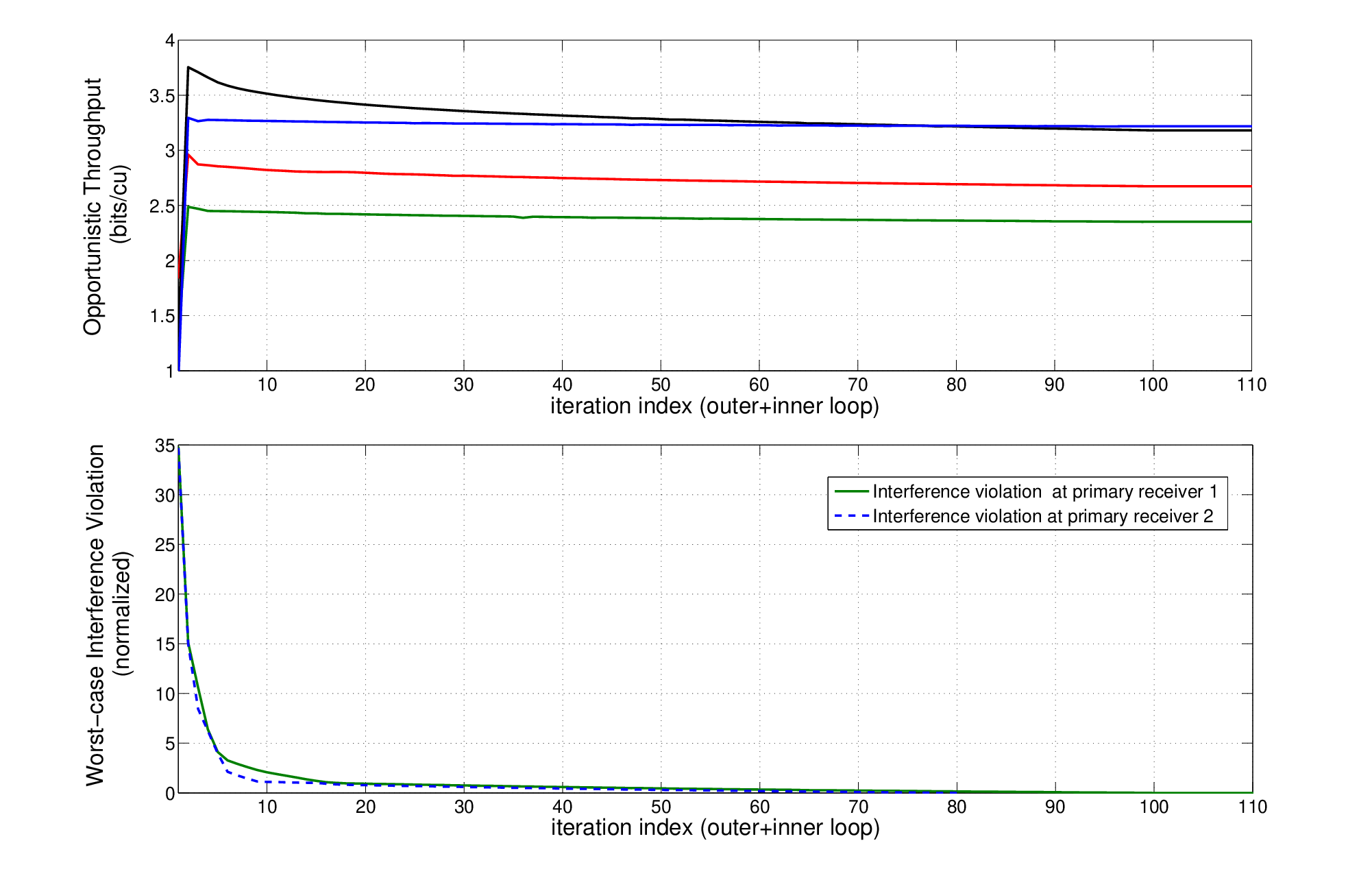
7 Conclusions
In this paper, we proposed a novel class of noncooperative games with (possibly) side constraints, where each SU aims to maximize his own opportunistic throughput by choosing jointly the sensing duration, the detection thresholds, and the vector power allocation over SISO frequency-selective interference channels, under local and (possibly) global average probabilistic interference constraints. In particular, to enforce global interference constraints while keeping the optimization as decentralized as possible, we proposed a pricing mechanism that penalizes the SUs in violating the global interference constraints. The proposed games belong to the class of nonconvex games and lack boundedness in some of the optimization variables, which makes the analysis quite involved. A major contribution of this paper was to introduce a new methodology for studying the existence and the uniqueness of the solution of nonconvex games with side constraints and design distributed solution algorithms. The proposed class of algorithms spans from noncooperative settings modeling selfish users to cooperative scenarios where the users are willing to exchange limited signaling (in the form of consensus algorithms) in favor of better performance. Numerical results showed the superiority of the proposed design (in terms of achievable system throughput) with respect to the state-of-the-art centralized and decentralized resource allocation algorithms for CR systems. Together with their fast convergence behavior, this makes them appealing in many practical CR scenarios.
Appendix
Appendix A Proof of Proposition 2
A.1 Intermediate results
To prove the proposition we need two intermediate results, stated in Lemma 11 and Lemma 12 below. Lemma 11 proves that the Abadie Constraint Qualification (ACQ) holds true at every (nontrivial) optimal solution of (32), which implies that any of such solutions must satisfy the KKT conditions associated with (32). Lemma 12 proves the boundedness of the multipliers associated with the local nonconvex constraint at any solution of (32).
Lemma 11.
The ACQ holds at every feasible solution of problem (32).
Proof.
The proof follows similar steps of [26, Prop. 8] and thus is omitted. ∎
Lemma 12.
Proof.
First of all, observe that the nonconvex problem (32) admits a solution , for every given and ; by Lemma 11, must satisfy the KKT conditions of the problem, for some multipliers associated with the constraint . Given the KKT conditions (which are omitted here), starting from the complementarity of the -variables, summing over , and invoking the orthogonality condition, we obtain: denoting by and the multipliers associated to the power budget and the spectral mask constraints, respectively,
| (69) |
where in the last inequality we used the following property of the logarithmic function, which is an immediate consequence of its concavity: for any scalar and , it holds that for all Inequality in (69) together with the complementarity conditions associated to the power constraints and , and the individual nonconvex interference constraint lead to
| (70) |
The desired result follows from (70) and for . ∎
A.2 Proof of Proposition 2
The proof is organized in the following two steps:
Step 1. We show first that under the assumptions in the proposition, each problem (32) has a unique optimal solution, for any given .
Step 2. Then, we prove that any optimal solution of (32) is nontrivial.
Step 1. Given and , let be a solution of (32); by Lemma 11, there exists a multiplier such that satisfies the VI in (40); by Lemma 12, it must be . It turns out that to prove Proposition 2 is sufficient to show that, under the condition in the proposition, the VI has a unique solution in the -variables.
Suppose by contradiction that there are two distinct solutions of the VI, denoted by and , with . Then, we have
Summing the two inequalities yields to
| (71) |
Invoking the mean-value theorem applied to to the univariate, differentiable, scalar-valued function
| (72) |
we deduce that there exists some , such that (71) can be written as
| (73) | |||||
| (74) | |||||
| (82) |
where in (73) denotes the Jacobian matrix of with respect to . Since (recall that is a convex set) and , the inequality in (82) contradicts the positive definiteness of , as assumed in Proposition 2.
Step 2. To complete the proof it is enough to show that the -component of any optimal solution of (32) is such that is lower bounded by a positive constant; see Lemma 13 below. To state the lemma, we need the following intermediate definitions. Let be any tuple such that
| (83) |
so that for all pairs satisfying (12)(b), the interference constraints (12)(a) evaluated at hold; and let
| (84) |
Note that, under the feasibility conditions (25), such a satisfies [see (12)(b)]
| (85) |
for any . Finally, given , let
| (86) |
We can now introduce Lemma 13 that provides a lower bound for the optimal sum-power allocation of each player.
Lemma 13.
Given , and feasible , and for all , the power-part of any optimal solution of the -th nonconvex optimization problem in (12) satisfies
| (87) |
Proof.
Let , , with , and for satisfying be given. Let define ; we then have . Therefore, if is player ’s best-response corresponding to , and , then
| (88) |
where and are defined in (5) and (6), respectively. On the other end, we have:
| (89) |
with defined in (86), and in (89) we used and . The desired bound in (87) follows readily from (88) and (89).∎
Appendix B Proof of Corollary 3
The proof is based on the following two steps.
Step 1. We introduce a symmetric matrix, denoted by , having the property that: given ,
| (90) |
which guarantees that is positive definite if is so.
Step 2. We derive sufficient conditions for to be positive definite.
Step 1. It is not difficult to see that (90) is satisfied if is built such that: for all ,
| (91) |
To construct such a matrix, we need to bound properly the entries of . Recalling that has the following expression [cf. (41)]:
| (92) |
we focus next on each term in (92) separately.
| (94) |
with
| (95) | ||||
| (96) | ||||
| (97) |
We provide now some bounds of the above quantities that will be used to define the diagonal entries of . The minimum eigenvalue of the positive definite matrix is lower bounded by: for all ,
| (98) |
whereas a lower bound of the first and last diagonal elements in (94) are: for all feasible [see conditions (b) and (c) in (12)],
| (99) |
where we used the following lower bound of : This bounds will be used to define the diagonal entries of the candidate matrix .
Matrix . Let introduce first the following quantities and their associated bounds:
| (100) |
| (101) |
| (104) |
which can be collected in the vectors , , , and , , . Finally, we introduce the column vector of the cross-channel transfer function between the secondary transmitter and the PU, and the notation for given and . Then, matrix can be written as
| (105) |
Based on (105), let us introduce the matrix obtained from by setting to zero the diagonal terms ( denotes the off-diagonal part of the matrix ) and take an upper bound of its off-diagonal entries (the inequalities below have to be intended component-wise):
| (106) |
Matrix . Following similar steps as for (106), we obtain
| (107) |
We are now ready to introduce the matrix satisfying (91). Given , and the definitions in (100)-(B) and (107), we define
| (108) |
Step 2. It follows from Step 1 that in (108) satisfies the desired property (90). Condition (43) of the corollary is readily obtained by imposing that is row-diagonal dominant, and setting
| (109) |
Appendix C Proof of Theorem 5
To prove the theorem we need the following lemma whose proof follows the same idea of that in Lemma 12 and thus is omitted.
Lemma 14.
Proof of Theorem 5. We prove only statement (a); the proof of the second part (b) follows similar steps of those in the proof of Proposition 2 and thus is omitted. Given , under the assumptions in (a), Proposition 4 states that the game admits a nontrivial NE ; by Lemma 11, there exist multipliers such that satisfies the VI in (45) [or equivalently (44)]. Lemma 14 shows that the upper bound constraint on the price in is not binding at , implying from iii) of (44) that and thus . Hence, must be a NE of the original un-truncated game [recall that, under the positive definiteness of the matrices on , each optimization problem in (32), with and , has a unique stationary (and thus optimal) solution, which then must be equal to ; see Proposition 2].
Appendix D Proof of Corollary 6
In order to obtain more general conditions than those in Theorem 5, by Lemma 13, we can restrict the check of the positive definiteness of the matrices and as required in Theorem 5 to the subset of the feasible set where any solution of the game lies. More specifically, let us introduce the restriction of the sets and defined in (4) and (19), respectively, to the power allocations satisfying (87): given ,
| (110) | ||||
| (111) |
where is defined as in (19), but with replaced by . By Lemma 13, instead of checking the positive definiteness of and on the feasible set , we can restrict this requirement to the subset .
We can now prove the corollary. We show next that (47) are sufficient conditions for the matrix to be positive definite on . Fist of all, observe that matrix can be written as
where . Since the matrix in (D) is positive semidefinite, we can focus only on . To obtain a sufficient condition for to be positive definite on , we follow a similar idea of that in Corollary 3. Namely, we build a proper matrix such that, for some ,
| (117) |
To this end, we focus on each term in (D) separately and derive proper bounds.
Matrix . Recalling the definition of , with given in (6), we have
| (118) |
with
| (119) |
given in (95) and
| (120) | ||||
| (121) |
Using the following lower bound for the rate function : given and ,
| (122) | ||||
| (123) |
where the second inequality follows from Lemma 13, we have for : given , and with ,
| (124) |
which leads also to
| (125) |
Using defined in (108), we are now ready to introduce the matrix , defines as: given ,
| (126) |
which satisfies the desired property in (117).
A sufficient condition for (117) can be obtained as in (47), by imposing that (the symmetric part of) is row diagonal dominant. More specifically, introducing
| (127) |
the diagonal dominance conditions is: for each and ,
| (128) |
After substituting the explicit expression of and doing some manipulations, (128) leads to the desired condition (47), where we defined as
| (129) |
with given in (109) and
| (130) |
Appendix E Convergence of Asynchronous Best-Response Algorithms for
In this section, we study the convergence of asynchronous best-response algorithms solving the game in (48); an instance of such algorithms is represented by Algorithm 5.1. Since the study of convergence is based on contraction arguments of the best-response map associated with game , we derive first sufficient conditions for this best-response to be a contraction; see Sec. E.1. We then provide the main theorem stating convergence of the asynchronous best-response algorithms; see Sec. E.2.
E.1 Contraction properties of the best-response of
Before introducing the main result of this section, we need the following intermediate definitions. Given defined in (37), let be the matrix, defined as
| (131) |
where and denote the spectral norm of and the minimum eigenvalue of the symmetric matrix , respectively. Given and as defined in (110) (cf. Appendix D), we also introduce
| (132) |
and the diagonal matrices and
| (133) |
with defined in (17). Given the coefficients
| (134) |
for and we can finally define the matrix that plays a key role in studying contraction properties of the best-response map associated with the game :
| (135) |
It is important to remark here that the off-diagonal entries of the matrix depend, among other quantities, on the cross-channels and . Roughly speaking, this dependence is such that the ’s tend to decrease as the aforementioned cross-channels decrease, meaning that the remains “small” as long as the overall MUI in the system remains “small”. We will show shortly that this is what one needs to guarantee the convergence of the distributed best-response based algorithms introduced in Sec. 5.1. More formally, by postulating that is a P-matrix, Theorem 15 below states the contraction properties of the best-response mapping of the game with respect to the suitably defined block maximum norm [see proof of the theorem for details].
Theorem 15.
Given the game with exogenous (fixed) price , suppose that in (135) is a P-matrix. Then the following hold:
- (a)
-
Each nonconvex optimization problem in (48) has a unique (nontrivial) optimal solution , for every given and ;
- (b)
-
The best-response map is a block-contraction; the unique fixed-point of is the unique -component of the NE of the game.
Proof.
To prove contraction of the best-response, we need to specify first under which norm the best-response map contracts. We will use the following norms: the block-maximum norm on defined as [42]
| (136) |
where is a valid vector norm on and is any given positive weight vector. In particular, we choose as follows: partitioning the vector as , with (or ) being the -length vector containing the last components (or the first component) of , and given the matrix as defined in (133), let the vector norm be , where . As it will be clarified shortly, the choice of such a norm is instrumental to obtain convergence conditions that can be satisfied for all ranges of . We also need to introduce the (weighted) maximum norm on defined as [49]
| (137) |
and the matrix norm on induced by given by [49]
| (138) |
We are now ready to prove the theorem.
(a): Given , the P property of matrix implies for all , and thus for all , , and . According to Proposition 2, this guarantees the uniqueness of the optimal solution of each nonconvex problem in (48), for every given and .
(b): Given the unique solution , by Lemma 11, it follows that there exists a multiplier associated with the nonconvex constraint such that the tuple satisfies the KKT optimality conditions of the optimization problem in (48), or equivalently, the VI defined in (40), which we rewrite here for the reader’s convenience:
| (139) |
with defined in (37). Recall that (Lemma 12) and (Lemma 13).
Consider now two feasible points , with for , and , and let ’s be the multipliers associated with the nonconvex constraints ’s at the optimal solutions , for . Evaluating (139) first in the solution given , then in the solution given , and summing the resulting inequalities, we obtain
| (140) |
By the main-value theorem we deduce that there exists a and a pair such that
| (141) | |||||
Using the definition of , , , and and as given in (131), (132), (133), and (125), respectively, let us introduce for each , the error vectors:
| (142) |
and the matrices
and
where the upper bound in (E.1) follows from Lemma 13 and (125). Then, from inequality (141), we deduce
| (153) |
which, using the bounds in (E.1) and (E.1) and the definition of in (134), leads
| (154) |
for all (the inequality in (141) is trivially satisfied if ). Introducing the vectors and , and the matrix , the set of inequalities in (154) can be written in vectorial form as
| (155) |
and thus, for any given , we have
| (156) |
for all . To complete the proof we need to show that for some . Invoking Lemma [34, Lemma 5.2.14] and [42, Cor. 6.1], we obtain the desired result:
| (157) |
∎
E.2 Asynchronous convergence theorem
Convergence of best-response algorithms solving the game follows readily from the block-contraction properties of the best-response, as proved in Theorem 15 and is thus guaranteed under the same conditions given in Theorem 15.
Theorem 16.
Given the game with exogenous (fixed) , suppose that in (135) is a P-matrix. Then, any sequence generated by the asynchronous algorithm based on the best-response and starting from any point in converges to a NE of the game, for any given updating feasible schedule of the players.
E.3 On the contraction/convergence conditions
We derive here easier conditions to be checked implying those in Theorem 16 (and Theorem 15); this sheds light also on their physical interpretation. The approach is similar to that followed to prove Corollary 6; we thus provide only a sketch of the proof.
The main idea is to build a matrix, say , such that [the inequality has to be intended component-wise], implying that if is a P matrix, then is so [34], which is the condition required by Theorem 16. Then, we provide sufficient conditions for to be a P matrix.
To obtain such a , it is sufficient to properly upper bound (the modulus of) the off-diagonal entries of . Given the expression of [cf. (134)], a way to do that is to find a matrix such that , and a diagonal matrix such that , where and are defined in (131) and (133), respectively. Skipping tedious intermediate derivations, we obtain the following
| (158) |
where is defined in (99), denotes the -dimensional lower right block of the matrix defined in (108), and is given by
| (159) |
with and defined in (100) and (B), respectively. Note that, since the following bounds hold between the entries of and :
matrix satisfies the desired property .
Finally, using , we can introduce a lower bound of the quantities in (132)
| (160) |
and define the matrix as
| (161) |
which satisfies . Using the above matrices, the desired upper bound of the coefficients is
| (162) |
with and defined in (125) and (E.1), respectively. Using these quantities it is not difficult to see that the matrix defined as
| (163) |
satisfies the desired property for any .
Since is a P matrix if and only if [34, Lemma 5.2.14], imposing that is row or column diagonal dominat, leads to the desired sufficient conditions guaranteeing convergence of asynchronous algorithms based on the best-response . This is made formal in the corollary below.
Corollary 17.
Statements in Theorem 16 (or Theorem 15) hold true if one of the two following conditions is satisfied:
- Low received MUI: for all ,
| (164) |
- Low transmitted MUI: for all ,
| (165) |
The physical interpretation of the above conditions is similar to that given for the existence/uniqueness of the NE (cf. Section 4.3). Roughly speaking, conditions (164) or (165) require “low” interference in the network, meaning “small” values of the (normalized) cross-channels as well as large values of coefficients , which is met if, among all, the (normalized) cross-channels are “sufficiently small”. An illustrative example is obtained in the two opposite cases where there is no optimization of the sensing times (and thus ) or the sensing times are optimized by imposing a common optimal sensing time by choosing a (sufficiently) large constant (and there are many active SUs). For those two cases, conditions (164) and (165) reduce respectively to
| (166) |
with
Note that ’s, among all, depend on the cross-channels , and become “small” when are small. Conditions (166) are thus satisfies if there is not “too much” interference in the system.
Appendix F Convergence of Best-Response Algorithms for
F.1 Proof of Theorem 10
First of all note that, given and and under the setting of Lemma 7, the game has a unique NE, denoted by , where we made explicit the dependence on the regularization tuple . This makes the sequence generated by Algorithm 5.2 well defined. The uniqueness of the NE of can be proved by exploring the connection between the game and a suitably defined VI, as briefly outlined next. Under the positive definiteness of matrix (as required by Lemma 7), is equivalent to the , with given in (45) and the VI function defined as
| (167) |
In other words, the is obtained by the in (45) introducing the proximal regularization of some of the VI variables, namely the -variables and -variable. The Jacobian matrix of denoted by is
| (168) |
where . If is uniformly positive definite, then so is . It turns out that, under the setting of Lemma 7, the regularized VI is strongly monotone [35, Prop. 2.3.2(c)] and thus has a unique solution [35, Th. 2.3.3], implying the uniqueness of the NE of .
Once we have proved that is well defined for any given and , we can derive the main properties of such a tuple [interpreting its components as functions of ], along with its connection with the NE of the game [and thus ]; these properties will be instrumental to prove Theorem 10.
Proposition 18.
Given , suppose that in (46) is uniformly positive definite for all , and let be given. Then the following hold:
- (a)
-
The mapping associated with the -components and -component of , i.e.,
(169) has a fixed point, and it is nonexpansive on ;
- (b)
-
The mapping associated with the -components of , i.e.,
(170) is Lipschitz continuous on , i.e., there exists a constant such that
(171) for all ;
- (c)
-
For any fixed-point of , the tuple is a solution of the ; therefore, it is a NE of .
Proof.
We prove next only (a) and (b); (c) follows similarly.
(a) Let be a solution of the in (45), whose existence is guaranteed by Lemma 7; recall that, by Lemma 12, it must be . It follows that: i) is the unique solution of the ; and ii) is also a solution of . Hence, it must be , , and , which implies the existence of a fixed-point of the mapping in (169); moreover, since , such a fixed point is in .
We prove now that is nonexpansive on . Given two distinct tuples , by definition, the tuples , with , satisfy the following:
| (172) |
for all and . Thus, similar to the proof of Theorem 15, we deduce
| (173) |
By the mean-value theorem, it follows that there exists a tuple lying on the line segment joining and such that [see also (168)]
Applying the Cauchy–Schwartz inequality and reorganizing terms we obtain:
where the last inequality follows from the positivity of the quadratic form, due to the positive definiteness of ; which proves the desired nonexpansive property of the mapping :
| (180) |
(b) Following similar steps as in (a) and using the Cartesian structure of the set we deduce that, for any given , there exists a tuple lying on the segment joining and such that
| (181) |
where the last inequality follows from the Cauchy–Schwartz inequality and the nonexpansive property of [cf. (180)], and . Invoking the uniform positive definiteness of and the boundedness of the set , we deduce from (181)
| (182) |
for some finite positive , which proves the desired Lipschitz continuity of on .∎
Proof of Theorem 10. We are now ready to prove the theorem. The outer loop of Algorithm 10 [see (62) in Step 3] is an instance of the Jacobi Over Relaxation, JOR, method [50] applied to the mapping ; which, using the notation introducing above, can be equivalently rewritten as:
| (183) |
Since is nonexpansive on [Proposition 18(a)], the sequence generated by the JOR scheme (183) converges to a fixed-point of [50, Th. 12.3.7]. By Proposition 18(b) [see (171)], the convergence of implies also the convergence of the sequence in the inner loop of Algorithm 10 to ; the limit point is the claimed NE of [Proposition 18(c)], and thus , if (Theorem 5).
References
- [1] Z. Quan, S. Cui, H. V. Poor, and A. H. Sayed, “Collaborative wideband sensing for cognitive radios: An overview of challenges and solutions,” IEEE Signal Processing Magazine, vol. 25, no. 6, pp. 60–73, Nov. 2008.
- [2] ——, “Optimal multiband joint detection for spectrum sensing in cognitive radio networks,” IEEE Trans. on Signal Processing, vol. 57, no. 3, pp. 1128–1140, March 2009.
- [3] Y.-C. Liang, Y. Zeng, E. C. Y. Peh, and A. T. Hoang, “Sensing-throughput tradeoff for cognitive radio networks,” IEEE Trans. on Wireless Communications, vol. 7, no. 4, pp. 1326–1337, April 2008.
- [4] P. Paysarvi-Hoseini and N. Beaulieu, “Optimal wideband spectrum sensing framework for cognitive radio systems,” IEEE Trans. on Signal Processing, vol. 59, no. 3, pp. 1170–1182, March 2011.
- [5] F. Rongfei and J. Hai, “Optimal multi-channel cooperative sensing in cognitive radio networks,” IEEE Trans. on Wireless Communications, vol. 9, no. 3, pp. 1128–1138, March 2010.
- [6] S.-J. Kim and G. B. Giannakis, “Rate-optimal and reduced-complexity sequential sensing algorithms for cognitive ofdm radios,” EURASIP Jour., Adv. Sig. Proc., Special Issue on Dynamic Spectrum Access for Wireless Networking, vol. 2009, Sept. 2009.
- [7] S. Barbarossa, S. Sadellitti, and G. Scutari, “Joint optimization of detection thresholds and power allocation for opportunistic access in multicarrier cognitive radio networks,” in Proc. of the IEEE Third International Workshop on Computational Advances in Multi-Sensor Adaptive Processing (CAMSAP 2009), Radisson Aruba Resort, Casino Spa Aruba, Dutch Antilles, USA, December 13-16 2009.
- [8] Y. Pei, Y.-C. Liang, K. C. Teh, and K. H. Li, “How much time is needed for wideband spectrum sensing?” IEEE Trans. on Wireless Communications, vol. 8, no. 11, pp. 5466–5471, November 2008.
- [9] S. Barbarossa, S. Sadellitti, and G. Scutari, “Joint optimization of detection thresholds and power allocation in multiuser wideband cognitive radios,” in Proc. of Cognitive Systems with Interactive Sensors (COGIS 2009), Paris, France, Nov. 16-18 2009.
- [10] X. Huang and B. Beferull-Lozano, “Non-cooperative power allocation game with imperfect sensing information for cognitive radios,” in Proc. of the IEEE International Conference on Acoustics, Speech, and Signal Processing (ICASSP 2011), Prague, Czech Republic, May 22-27 2011.
- [11] Y. Xing, C. N. Mathur, M. Haleem, R. Chandramouli, and K. Subbalakshmi, “Dynamic spectrum access with QoS and interference temperature constraints,” IEEE Trans. on Mobile Computing, vol. 6, no. 4, pp. 423–433, April 2007.
- [12] Q. Lu, W. Wang, W. Wang, and T. Peng, “Asynchronous distributed power control under interference temperature constraints,” in Proc. of the IEEE Global Telecommunications Conference (GLOBECOM), New Orleans, LA, USA, Nov. 30-Dec. 4 2008.
- [13] W. Wang, T. Peng, and W. Wang, “Optimal power control under interference temperature constraints in cognitive radio network,” in Proc. of the IEEE Wireless Communications and Networking Conference (WCNC 2007), Hong Kong, HK, March 11-15 2008.
- [14] D. Schmidt, C. Shi, R. Berry, M. Honig, and W. Utschick, “Distributed resource allocation schemes: Pricing algorithms for power control and beamformer design in interference networks,” IEEE Signal Processing Magazine, vol. 26, no. 5, pp. 53–63, Sept. 2009.
- [15] Z.-Q. Luo and S. Zhang, “Spectrum management: Complexity and duality,” Jour. of Selected Topics in Signal Processing, vol. 2, no. 1, pp. 57–72, Feb. 2008.
- [16] W. Yu and R. Lui, “Dual methods for nonconvex spectrum optimization of multicarrier systems,” IEEE Trans. on Communications, vol. 54, no. 7, pp. 1310–1322, July 2006.
- [17] M. Rossi, A. M. Tulino, O. Simeone, and A. M. Haimovich, “Nonconvex utility maximization in gaussian miso broadcast and interference channels,” in Proc. of the International Conference on Acoustics, Speech and Signal Processing (ICASSP 2011), Prague, Czech Republic, March 22-27 2011.
- [18] Z.-Q. Luo and J.-S. Pang, “Analysis of iterative waterfilling algorithm for multiuser power control in digital subscriber lines,” EURASIP Jour. on Applied Signal Processing, vol. 2006, pp. 1–10, May 2006.
- [19] G. Scutari, D. P. Palomar, and S. Barbarossa, “Optimal linear precoding strategies for wideband noncooperative systems based on game theory—part III: Nash equilibria and distributed algorithms,” IEEE Trans. on Signal Processing, vol. 56, no. 3, pp. 1230–1267, March 2008.
- [20] ——, “Asynchronous iterative water-filling for Gaussian frequency-selective interference channels,” IEEE Trans. on Information Theory, vol. 54, no. 7, pp. 2868–2878, July 2008.
- [21] J.-S. Pang, G. Scutari, D. P. Palomar, and F. Facchinei, “Design of cognitive radio systems under temperature-interference constraints: A variational inequality approach,” IEEE Trans. on Signal Processing, vol. 58, no. 6, pp. 3251–3271, June 2010.
- [22] G. Scutari, D. P. Palomar, F. Facchinei, and J.-S. Pang, “Monotone games for cognitive radio systems,” in Distributed Decision-Making and Control, A. Rantzer and R. Johansson, Eds. New York: Lecture Notes in Control and Information Sciences Series, Springer Verlag, 2011.
- [23] H. Mohsenian-Rad, J. Huang, M. Chiang, and V. W. Wong, “Utility optimal random medium access control: Reduced complexity, fast convergence, and robust performance,” IEEE Trans. on Wireless Communications, vol. 8, no. 2, pp. 2984–2993, Feb. 2009.
- [24] A. Leshem and E. Zehavi, “Game theory and the frequency selective interference channel,” IEEE Signal Processing Magazine, vol. 26, no. 5, pp. 28–40, September 2009.
- [25] E. Larsson, E. Jorswieck, J. Lindblom, and R. Mochaourab, “Game theory and the flat-fading gaussian interference channel,” IEEE Signal Processing Magazine, vol. 26, no. 5, pp. 18–27, September 2009.
- [26] J.-S. Pang and G. Scutari, “Nonconvex cognitive radio games: Quasi-Equilibria,” IEEE Trans. on Signal Processing, (to appear) 2013.
- [27] J. Rosen, “Existence and uniqueness of equilibrium points for concave n-person games,” Econometrica, vol. 33, no. 3, pp. 520–534, July 1965.
- [28] M. J. Osborne and A. Rubinstein, A Course in Game Theory. MIT Press, July 2004.
- [29] M. R. Baye, G. Tian, and J. Zhou, “Characterizations of the existence of equilibria in games with discontinuous and non-quasiconcave payoffs,” The Review of Economic Studies, vol. 60, no. 4, pp. 935–948, Oct. 1993.
- [30] B. Corneta and M.-O. Czarnecki, “Existence of generalized equilibria,” Nonlinear Analysis, vol. 44, pp. 555–574, 2001.
- [31] J.-S. Pang and G. Scutari, “Nonconvex games with side constraints,” SIAM Jour. on Optimization, vol. 21, no. 4, pp. 1491–1522, Dec. 2011.
- [32] G. Scutari, D. Palomar, F. Facchinei, and J.-S. Pang, “Convex optimization, game theory, and variational inequality theory in multiuser communication systems,” IEEE Signal Processing Magazine, vol. 27, no. 3, pp. 35–49, May 2010.
- [33] G. Scutari, F. Facchinei, J.-S. Pang, and D. P. Palomar, “Real and complex monotone communication games,” IEEE Trans. on Information Theory, (submitted) 2012. [Online]. Available: http://arxiv.org/abs/1212.6235.
- [34] R. W. Cottle, J.-S. Pang, and R. E. Stone, The Linear Complementarity Problem. SIAM Classics in Applied Mathematics 60, Philadelphia (2009) [Originally published by Academic Press, Boston (1992)].
- [35] F. Facchinei and J.-S. Pang, Finite-Dimensional Variational Inequalities and Complementarity Problem. Springer-Verlag, New York, 2003.
- [36] ——, “Nash equilibria: The variational approach,” in Convex Optimization in Signal Processing and Communications, D. P. Palomar and Y. C. Eldar, Eds. London: Cambridge University Press, 2009.
- [37] A. Berman and R. J. Plemmons, Nonnegative Matrices in the Mathematical Sciences. Society for Industrial Mathematics (SIAM), 1987.
- [38] G. Scutari and J.-S. Pang, “Joint sensing and power allocation in nonconvex cognitive radio games: Quasi-nash equilibria,” in Proc. of the 17th International Conference on Digital Signal Processing (DSP2011), Corfu, Greece, July 6-8 2011.
- [39] S. Zlobec, Stable Parametric Programming. Kluwer Academic Publishers, 2001.
- [40] R. Cendrillon, J. Huang, M. Chiang, and M. Moonen, “Autonomous spectrum balancing for digital subscriber lines,” IEEE Trans. on Signal Processing, vol. 55, no. 8, pp. 4241–4257, Aug. 2007.
- [41] G. Scutari, D. Palomar, F. Facchinei, and J.-S. Pang, “Flexible design of cognitive radio wireless systems: From game theory to variational inequality theory,” IEEE Signal Processing Magazine, vol. 26, no. 5, pp. 107–123, September 2009.
- [42] D. P. Bertsekas and J. N. Tsitsiklis, Parallel and Distributed Computation: Numerical Methods, 2nd ed. Athena Scientific Press, 1989.
- [43] S. Barbarossa and S. Sadellitti, “Joint optimization of sensing and radio resource allocation in collaborative femtocell networks,” in Proc. of the 3rd International Workshop on Cognitive Information Processing (CIP 2012), Baiona, Spain, 28-30 May 2012.
- [44] J. N. Tsitsiklis, “Problems in decentralized decision making and computation,” Ph.D. dissertation, Massachussetts Istitute of Technology, 1984.
- [45] R. Olfati-Saber, J. A. Fax, and R. M. Murray, “Consensus and cooperation in networked multi-agent systems,” Proceedings of the IEEE, vol. 95, no. 1, pp. 215–223, Jan. 2007.
- [46] G. Scutari, S. Barbarossa, and L. Pescosolido, “Distributed decision through self-synchronizing sensor networks in the presence of propagation delays and asymmetric channels,” IEEE Trans. on Signal Processing, vol. 56, no. 4, pp. 1667–1684, April 2008.
- [47] S. Sundaram and C. N. Hadjicostis, “Distributed function calculation and consensus using linear iterative strategies,” IEEE Jour. on Selected Areas in Communications, vol. 26, no. 4, pp. 650–660, May 2008.
- [48] M. Chiang, P. Hande, T. Lan, and C. W. Tan, Power control in wireless cellular networks. Foundations and Trends in Networking, Now Publishers, July 2008, vol. 2, no. 4.
- [49] R. A. Horn and C. R. Johnson, Matrix Analysis. Cambridge University Press, 1985.
- [50] J. M. Ortega and W. C. Rheinboldt, Iterative Solution of Nonlinear Equations in Several Variables. Society for Industrial Mathematics (SIAM), Phila, USA, 1987.