Perturbative stability of catenoidal soap films

Soumya Jana Note: Electronic address: soumyajana.physics@gmail.com Affiliation: Department of Physics
Indian Institute of Technology, Kharagpur 721 302, India Sayan Kar Note: Electronic address: sayan@iitkgp.ac.in Affiliation: Department of Physics and Centre for Theoretical Studies
Indian Institute of Technology, Kharagpur 721 302, India

Abstract

The perturbative stability of catenoidal soap films formed between parallel, equal radii, coaxial rings is studied using analytical and semi-analytical methods. Using a theorem on the nature of eigenvalues for a class of Sturm–Liouville operators, we show that for the given boundary conditions, azimuthally asymmetric perturbations are stable, while symmetric perturbations lead to an instability–a result demonstrated in Ben Amar et. al [7] using numerics and experiment. Further, we show how to obtain the lowest real eigenvalue of perturbations, using the semi-analytical Asymptotic Iteration Method (AIM). Conclusions using AIM support the analytically obtained result as well as the results in [7]. Finally, we compute the eigenfunctions and show, pictorially, how the perturbed soap film evolves in time.

I Introduction

Soap films and bubbles have, over the years, been a topic of active interest both in pedagogy and in research, in mathematics as well as in physics. In the eighteenth and nineteenth century, it was Lagrange [1] and Plateau [2] who pioneered the study of such minimal surfaces which eventually led to the well-known Plateau problem in mathematics. Plateau, in fact was also the first to perform a series of elegant experiments with soap films which served as a basis for future experimental and mathematical investigations. Further details on the science of soap films and bubbles from a physicists’ viewpoint can be found in the well-known book of Isenberg [3]. On the mathematical front, the book by Osserman [4], as its title suggests, provides a survey on minimal surfaces.

Our interest in this article is focused on one specific soap film configuration–the film formed between a pair of parallel, coaxial, equal radii rings (see Fig. 1). Geometrically, we know that the surface spanned by the film is a catenoid–a minimal (zero mean curvature) surface. Following original work by Plateau, an extensive analysis on this class of films was done in 1980 by Durand [5]. More recently, some theoretical and experimental work has been reported in [6].

Refer to caption — Figure 1: In the left figure, a rough sketch of a catenoidal soap film suspended between two coaxial circular rings of radius $r_{0}=a\cosh(\frac{h}{2a})$ , showing the parameters (the distance $h$ between the two rings and the minimum radius of the film $a$ ) [6]. In the right figure, a Mathematica 7.0 generated catenoid (with $h=2.0$ and $a=1.0$ ) is shown.

Finding the shape of such a soap film is a standard problem in the calculus of variations [8]. The shape is obtained by rotating a catenary curve about the vertical axis, to obtain a catenoidal surface of revolution. Mathematically, one first writes down the surface energy functional $V[S]$ for the soap film configuration, given as,

V[S]=2\pi\sigma\int^{h}_{0}r\sqrt{1+r_{z}^{2}}\,\,dz

(1)

where $r_{z}=\frac{dr}{dz}$ , $\sigma$ is the surface tension and $r(z)$ is the radius at an axial distance $z$ from the ring at $z=0$ (the other ring is at $z=h$ ). The Euler–Lagrange equation obtained from the first variation is then solved to find the surface.

An obvious and important question to ask is – what happens if we give a small perturbation about the extremal configuration? The catenoidal shape is sustained if the configuration is stable. If it is unstable, it collapses to two disconnected planar discs, which is also a solution of the Euler-Lagrange equation. To understand the stability question, which was discussed by Plateau and later in [5], we expand the surface energy functional about the extremal configuration in the following way :

V[S]=V[S_{0}]+\delta V[S_{0}]+\delta^{2}V[S_{0}]+.......

(2)

The different terms in the right hand side of the above equation are the zeroth, first and second variation terms. Setting the first variation term ( $\delta V[S_{0}]$ ) to zero gives the Euler-Lagrange equation which determines the extremal configuration. The next, second variation term $\delta^{2}V[S_{0}]$ , is crucial for us because it determines the stability of the film under perturbations.

In [5] it was shown how the second variation leads to an associated eigenvalue problem of the Sturm-Liouville type. Therefore, knowing the sign of the lowest eigenvalue would determine the stability of such soap films. If the lowest eigenvalue is negative then the catenoidal configuration is unstable. On the other hand, a positive lowest eigenvalue confirms its stability. Durand [5] analyzed in detail the stability question under azimuthally symmetric perturbations. Much later, in 1998, Ben Amar et. al [7] studied the stability and vibrations of catenoid-shaped smectic films, both numerically and experimentally. In our work, we confirm the results in [7] by using exclusively analytical and semi-analytical methods. We also trace the time evolution of the film and pictorially demonstrate our conclusions on stability.

II Eigenvalue equation for azimuthally asymmetric perturbation

The catenoidal configuration of the soap film suspended between two parallel, co-axial circular rings is described by the following equation of a catenary curve,

r(z)=a\cosh(\frac{z}{a}-\frac{h}{2a})

(3)

where, we have considered two rings of identical radius $r_{0}=a\cosh(\frac{h}{2a})$ . The azimuthally asymmetric perturbed configuration is described by,

f(z,\phi)=r(z)+g(z,\phi)

(4)

where $\phi$ is the azimuthal angle in the cylindrical co-ordinate system. $g(z,\phi)$ is the azimuthally asymmetric perturbation with boundary condition: $g(0,\phi)=g(h,\phi)=0$ and $g(z,\phi)=g(z,\phi+2\pi)$ .

The surface energy functional for this case comes from the following formula [6] for any general surface area (using cylindrical coordinates and ${\bf{f}}=(f(z,\phi)\cos\phi,f(z,\phi)\sin\phi,z)$ ),

S=\int|\frac{\partial{\bf{f}}}{\partial z}\times\frac{\partial{\bf{f}}}{\partial\phi}|d\phi dz

(5)

Thus we have,

V[S]=2\sigma\int^{h}_{0}\int^{2\pi}_{0}\sqrt{f^{2}(f_{z}^{2}+1)+f^{2}_{\phi}}d\phi dz

(6)

where, $f_{z}=\frac{\partial f}{\partial z}$ and $f_{\phi}=\frac{\partial f}{\partial\phi}$ . Hence, in this case, after a Taylor expansion of Eq. (6) about the extremal configuration (Eq. (3)) and performing the partial integration using the boundary conditions mentioned earlier, the second variation of the surface energy corresponding to the extremal surface $S_{0}$ becomes [5],

\delta^{2}V[S_{0}]=\sigma\int_{0}^{2\pi}\int_{-u_{0}}^{u_{0}}\frac{g_{u}^{2}+g_{\phi}^{2}-g^{2}}{\cosh^{2}u}dud\phi

(7)

where $u(z)=\frac{z}{a}-\frac{h}{2a}$ , ( $z[0,h]\longrightarrow u[-u_{0},u_{0}],u_{0}=\frac{h}{2a}$ ). The equations (5),(6) and (7) are also verified in detail using the general discussions on minimal surfaces given in [9].

$g(z,\phi)$ is related to the infinitesimal displacement $\xi(u)$ normal to the extremal surface of the film, by the following equation given in [5] ,

g(u,\phi)=\xi(u,\phi)\cosh(u)

(8)

Eq. (8) can be rewritten using $g(u,\phi)=g(u,\phi+2\pi)$ as,

g(u,\phi)=\zeta(u)\left(\begin{array}[]{c}\cos(m\phi)\\ \sin(m\phi)\end{array}\right)\cosh(u)

(9)

where $m=0,1,2,3.....$

The eigenvalue problem related to the second variation (Eq. (7)), as given in [5], is,

L\psi_{n}\equiv-\frac{d^{2}\psi_{n}}{du^{2}}+(m^{2}-\frac{2}{\cosh^{2}(u)})\psi_{n}=\lambda_{n}\cosh^{2}(u)\psi_{n}

(10)

where, $\psi_{n}$ , the eigen function of Sturm-Liouville operator $L$ , is related to $\zeta$ through the following equation,

\zeta(u)=\sum^{\infty}_{n=1}c_{n}\psi_{n}

(11)

As stated before, the stability of the soap film depends on the sign of the lowest eigenvalue $\lambda_{1}$ . In subsequent sections, we analyze the Eq. (10) both analytically and numerically in order to know about the nature of the eigenvalues and the eigenfunctions.

III A result on Sturm-Liouville operators

We now state a theorem from the literature [10] on Sturm–Liouville operators which we use later to learn about the nature of the eigenvalues.

Theorem : Let Eqs. (12) (see below) define a regular Sturm-Liouville problem, where Eq. (12a) is the eigenvalue equation, Eqs. (12b) and (12c) are general boundary conditions.

	$Lv:=-(p(x)v^{\prime})^{\prime}+q(x)v=\lambda w(x)v,\hskip 14.45377pta<x<b$		(12a)
	$B_{a}v:=A_{1}v(a)+A_{2}v^{\prime}(a)+a_{1}v(b)+a_{2}v^{\prime}(b)=0$		(12b)
	$B_{b}v:=b_{1}v(a)+b_{2}v^{\prime}(a)+B_{1}v(b)+B_{2}v^{\prime}(b)=0$		(12c)

$v^{\prime}=\frac{dv}{dx}$ . It is assumed that the interval $[a,b]$ is bounded (i.e. $-\infty<a<b<\infty$ ), the boundary conditions are linearly independent, all coefficients are real and the functions $p,p^{\prime},q,w$ are continuous in the domain $[a,b]$ . Also, $p(x)>0$ and $w(x)>0$ in $[a,b]$ . If the boundary conditions are separated (i.e. $a_{1}=a_{2}=b_{1}=b_{2}=0$ ) and $A_{1}A_{2}\leq 0$ and $B_{1}B_{2}\geq 0$ , then, using the Green’s identities [10, 11] for the Sturm-Liouville operator, we can show that for any eigenpair $(\lambda,v)$ ,

\lambda\geq\frac{min[q(x):a\leq x\leq b]}{max[w(x):a\leq x\leq b]}

(13)

For a proof of the above theorem see Appendix A.

Application:
In our problem, $x=u$ , $p(u)=1$ , $q(u)=-\frac{2}{\cosh^{2}(u)}+m^{2}$ , $w(u)=\cosh^{2}(u)$ , $a=-u_{0}$ , $b=u_{0}$ and boundary conditions are separated, with $A_{2}=B_{2}=0$ and $A_{1},B_{1}\neq 0$ . Therefore, our problem is a regular Sturm-Liouville problem satisfying the properties mentioned in the theorem quoted above. Thus, for $\lambda_{1}$ to be a negative eigenvalue, we need

min[q(u):-u_{0}\leq u\leq u_{0}]<0\Rightarrow\cosh^{2}(u_{0})<\frac{2}{m^{2}}

(14)

For $m=0$ , the above condition is always satisfied. If $m=1$ , we have, $1<\cosh^{2}(u_{0})<2$ . However, for the existence of a negative eigenvalue, $u_{0}$ must be greater than $1.2$ , since this is the critical value of $u_{0}$ for which the lowest eigenvalue $\lambda_{1}$ is zero, for $m=0$ . Only above this value of $u_{0}$ does $\lambda_{1}$ become negative for $m=0$ [5]. Note that $\cosh^{2}(1.2)=3.278$ . Thus, for $m=1$ , a negative eigenvalue does not exist. Further, for $m\geq 2$ , the inequality (14) becomes, $\cosh^{2}(u_{0})<\frac{1}{2}$ which is impossible because $\cosh^{2}(u_{0})\geq 1$ always. Therefore for all $m\geq 2$ , no negative eigenvalues exist.

The analysis above leads us to the result that, only the $m=0$ mode can be unstable.

IV Semi-analytical, numerical analysis

IV.1 Eigenvalues using AIM

The eigenvalues of the above Sturm-Liouville problem can be computed using the Asymptotic Iteration Method (AIM) for eigenvalue problems [12], which is briefly discussed in Appendix B. In our case the differential equation is,

\frac{d^{2}\psi_{n}}{du^{2}}+(\lambda_{n}\cosh^{2}u-m^{2}+\frac{2}{\cosh^{2}u})\psi_{n}=0

(15)

Since $\psi_{n}(-u_{0})$ = $\psi_{n}(u_{0})=0$ , $\psi_{n}(u)$ includes two factors which are $(u+u_{0})$ and $(u-u_{0})$ , the following transformation can be used for the present case,

\psi_{n}(u)=(u^{2}-u_{0}^{2})\varphi_{n}(u)

(16)

Using the above transformation in Eq. (15), we obtain the differential equation satisfied by $\varphi_{n}(u)$ ,

\frac{d^{2}\varphi_{n}}{du^{2}}=-\frac{4u}{u^{2}-u_{0}^{2}}\frac{d\varphi_{n}}{du}-(\frac{2}{u^{2}-u_{0}^{2}}+\lambda_{n}\cosh^{2}u-m^{2}+\frac{2}{\cosh^{2}u})\varphi_{n}

(17)

Comparing Eq. (17) with Eq. (41),using Eqs. (43), (44) and (45), we can calculate $\delta$ (see Appendix B for definition) and using a particular chosen value $u=u_{ch}$ between $-u_{0}$ to $u_{0}$ , $\delta$ becomes a function of $\lambda_{n}$ and finally, $\lambda_{n}$ can be computed by finding the roots of $\delta=0$ . In this case, while computing the eigenvalues $u_{ch}=0$ is used. In this way, eigenvalues were computed for different $u_{0}$ .

IV.2 Analytical check

The eigenvalue equation related to this problem can be solved analytically for two limiting cases of the $m=0$ mode. For this azimuthally symmetric case ( $m=0$ ), when $u_{0}\rightarrow u_{c}=1.2$ it is shown in [5] that,

	$\lambda_{1}\approx 3.598(\frac{h_{c}-h}{2r_{0}})^{\frac{1}{2}},\hskip 14.45377ptu_{0}<u_{c}$		(18a)
	$\lambda_{1}\approx-3.598(\frac{h_{c}-h}{2r_{0}})^{\frac{1}{2}},\hskip 14.45377ptu_{0}>u_{c}$		(18b)

Again if $u_{0}\rightarrow 0$ then,

\lambda_{1}\rightarrow(\frac{\pi}{2u_{0}})^{2}-2

(19)

Table 1: Comparison between the lowest eigenvalues for

m=0

mode obtained from Asymptotic Iteration Method using 16 iterations in Mathematica, with the analytical values from Eqs. (18)and (19)

$u_{0}\rightarrow u_{c}$			$u_{0}\rightarrow 0$
$u_{0}$	$\lambda_{1}$ (Eq. 18)	$\lambda_{1}$ (AIM)	$u_{0}$	$\lambda_{1}$ (Eq. 19)	$\lambda_{1}$ (AIM)
1.1	0.212	0.244	0.01	24672.01	24671.70
1.15	0.104	0.107	0.02	6166.50	6166.18
1.2	0.0	-0.01	0.03	2739.56	2739.23
1.25	-0.103	-0.114	0.04	1540.12	1539.80
1.30	-0.202	-0.210	0.05	984.96	984.64

The above check shown in Table 1 confirms that we can indeed use AIM to compute the eigenvalues for (Eq. (15)).

IV.3 Convergence of results in AIM

On performing the numerical calculations using AIM, we found that only 10 iterations were possible in Mathematica 7.0 in a 32-bit system. However, using the Improved Asymptotic Iteration Method (IAIM) (see Appendix B), 17 iterations could be carried out for the problem at hand. We noted that for higher value of $u_{0}$ , the results using 10 iterations are different from the results obtained from 16 iterations. This deviation increases with increasing $u_{0}$ . The reason is that 10 iterations are not sufficient to guarantee a convergence towards the result. We have inspected the convergence of our result for a number of iterations choosing $u_{0}=1.1$ . We note that the difference in results between 8th and 10th iteration is 0.06374, between 10th and 12th iteration it is 0.031732 , between 12th and 14th iteration it is 0.015443 and between 14th and 16th it is 0.007601. Thus, as the iteration number increases, the result converges more and more. After each iteration, $\eta$ or $s$ (see Appendix B for definition) become zero for $u_{ch}=0$ in an alternating fashion, resulting in the same lowest eigen value for two consecutive iterations. Therefore, we compare the $n$ th and the ( $n+2$ )th iterations. After 16 iterations, the result is seen to converge up to the second decimal point. If we wish to have even better convergence, we need to further increase the number of iterations.

However, let us inspect the same facts for $u_{0}=1.5$ (Table 2).

Table 2: Result of different number of iterations for finding the lowest real eigenvalue

\lambda_{1}

for

u_{0}=1.5,m=0

number of iterations	$\lambda_{1}$	number of iterations	$\lambda_{1}$
8	-0.756028	13	-0.704753
9	-0.756028	14	0.177329
10	0.448441	15	0.177329
11	0.448441	16	-0.660185
12	-0.704753	17	-0.660185

In this case the difference in results between 9th and 10th iteration is 1.204469, between 10th and 12th iteration is 1.153194, between 13th, 14th iteration it is 0.882082 and between 15th and 16th iteration it is 0.837514. We note that the result is indeed converging as the number of iterations increase. But, unlike the previous case (i.e. for $u_{0}=1.1$ ), where after 16 iterations, the result converged upto the second decimal point, we find that for $u_{0}=1.5$ the result does not converge even to the first decimal point! In addition, the difference between the results of 15th and 16th iteration is of the order of the actual eigenvalue. Clearly, for this case, we need a larger number of iterations to get the correct eigenvalue.

IV.4 A way to overcome the limitation of AIM

In the previous section, we have seen that for $u_{0}>1.2$ we need many more iterations than 16. However, using Mathematica we were unable to go beyond 17 iterations. In order to overcome this limitation, we have employed a heuristic approach which is elaborated in the Appendix C.

Using the combination of AIM and the above-stated method, we finally obtain the correct eigenvalues for $m=0$ . We have plotted $(\frac{\nu_{1}}{\pi})^{2}$ as a function of $\frac{h}{2r_{0}}$ in Fig. 2 (where , $\nu_{1}$ is the reduced frequency defined in [5]). Fig. 2 exactly matches with the plot shown in [5] (see Fig. 4 there). This ensures that our method is reliable and can be used to find the eigenvalues and analyse the stability of soap films between the two rings.

V Result of numerical analysis

In this section we discuss the plots for the lowest eigenvalues as a function $\frac{h}{2r_{0}}$ for different azimuthally asymmetric modes ( $m\neq 0$ ), where we have shown the behaviour for large $u_{0}$ . The plots in Fig. 3 show that only the $m=0$ plot goes below the zero eigenvalue line (it crosses the zero eigenvalue line at $u_{0}=1.2$ , alternatively $\frac{h}{2r_{0}}=0.663$ ). All other ( $m=1,2,3,4$ ) $m\neq 0$ curves asymptotically approach the zero value, for $u_{0}\rightarrow\infty$ or $\frac{h}{2r_{0}}\rightarrow 0$ . Thus, the result of numerical analysis agrees with the fact that only the $m=0$ mode can be unstable, a fact which we obtained analytically as well. This is the central result in our article.

VI Perturbed configurations

Let us now try and see if we can obtain the perturbed configurations and visualize their time evolution. If an infinitesimal displacement is given to the extremal configuration of the soap film which is described by Eq. 3, then the film will have a small motion about it. For the azimuthally symmetric case ( $m=0$ ) the general expression for the displacement about the extremal configuration, which describes this small motion of the soap film, is (given in [5]),

\xi(u,t)=\sum^{\infty}_{n=1}(a_{n}\cos(w_{n}t)+\frac{b_{n}}{w_{n}}\sin(w_{n}t))\psi_{n}(u)

(20)

where

a_{n}=\int^{u_{0}}_{-u_{0}}\psi_{n}(u)\xi(u,0)\cosh^{2}udu

(21)

b_{n}=\int^{u_{0}}_{-u_{0}}\psi_{n}(u)\xi_{t}(u,0)\cosh^{2}udu

(22)

w_{n}=(\frac{2\sigma}{\rho a^{2}}\lambda_{n})^{\frac{1}{2}}=(\frac{2\sigma}{\rho h^{2}})^{\frac{1}{2}}\nu_{n}

(23)

and $\xi_{t}=\frac{\partial\xi}{\partial t}$ . The frequency of oscillation $w_{n}$ is related to the dimensionless reduced frequency $\nu_{n}$ by Eq. (23), where $\rho$ is the mass of the film per unit area. If $u_{0}<u_{c}$ ( $u_{0}=\frac{h}{2a}$ and $u_{c}=\frac{h_{c}}{2a}=1.2$ corresponds to $\lambda_{1}=0$ ), then $w_{1}^{2}>0$ , consequently $w_{1}$ is real and the motion described by Eq. (20) is the small oscillation of the soap film about its stable configuration.

If $u_{0}>u_{c}$ , $w_{1}^{2}<0$ , $w_{1}$ is pure imaginary and the first term in Eq. (20) is hyperbolic,

\xi(u,t)=(a_{1}\cosh|w_{1}|t+\frac{b_{1}}{w_{1}}\sinh|w_{1}|t)\psi_{1}(u)+\sum^{\infty}_{n=2}(a_{n}\cos(w_{n}t)+\frac{b_{n}}{w_{n}}\sin(w_{n}t))\psi_{n}(u)

(24)

Thus, the first term grows in time and the configuration is unstable– it collapses into a configuration consisting of two plane discs.

Now if we consider an azimuthally asymmetric displacement, the expression for the displacement may be written as:

\xi(u,\phi,t)=\sum^{\infty}_{m=0}\sum^{\infty}_{n=1}(a_{mn}\cos(w_{mn}t+m\phi)+b_{mn}\sin(w_{mn}t+m\phi))\psi_{mn}(u)

(25)

where

a_{0n}=\frac{1}{2\pi}\int^{u_{0}}_{-u_{0}}\int^{2\pi}_{0}\xi(u,\phi,0)\psi_{0n}(u)\cosh^{2}u\,\,d\phi\,\,du

(26)

b_{0n}=\frac{1}{2\pi w_{n0}}\int^{u_{0}}_{-u_{0}}\int^{2\pi}_{0}\xi_{t}(u,\phi,0)\psi_{0n}(u)\cosh^{2}u\,\,d\phi\,\,du

(27)

a_{mn}=\frac{1}{\pi}\int^{u_{0}}_{-u_{0}}\int^{2\pi}_{0}\xi(u,\phi,0)\psi_{mn}(u)\cosh^{2}u\cos(m\phi)\,\,d\phi\,\,du

(28)

b_{mn}=\frac{1}{\pi}\int^{u_{0}}_{-u_{0}}\int^{2\pi}_{0}\xi(u,\phi,0)\psi_{mn}(u)\cosh^{2}u\sin(m\phi)\,\,d\phi\,\,du

(29)

In Eq. (25), the instability occurs only in the leading order term.

Using the eigenvalues obtained earlier, we solve Eq. (10) numerically and then plot the perturbed configurations. While plotting, we treat the eigenfunction itself as the perturbation, though in a real situation the perturbation is the linear combination of such eigenfunctions satisfying the same boundary condition.

Eq. (10), which is a second order differential equation can be written in terms of two first order differential equations in the following way:

\frac{d\zeta}{du}=\chi

(30)

\frac{d\chi}{du}=-(\lambda\cosh^{2}(u)-m^{2}+\frac{2}{\cosh^{2}(u)})\zeta

(31)

where, $\zeta\equiv\psi(u)$ . We solve the above two ordinary differential equations numerically using Mathematica with the initial conditions: $\zeta(-u_{0})=0$ and $\chi(-u_{0})$ (of arbitrary choice). Using the computed eigenfunction we evaluate the $g(u,\phi,t)$ via the following relation:

for the oscillating mode,

g(u,\phi,t)=\zeta(u)\cosh(u)cos(m\phi+w_{mn}t)

(32)

for the collapsing mode,

g(u,\phi,t)=\zeta(u)\cosh(u)\cosh(|w_{01}|t)

(33)

Finally, we plot the time evolution of the perturbed configuration using the following relation:

f(u,\phi,t)=r(u)+g(u,\phi,t)

(34)

In Fig. 4 and Fig. 5 we have shown the collapsing mode and oscillating mode respectively, where snapshots in time appear in each frame. The elapsed time mentioned in the figures are in units of $\frac{1}{\pi}\left(\frac{\rho h^{2}}{2\sigma}\right)^{\frac{1}{2}}$ . In Fig. 6, we have shown how the frequency of oscillation varies with the boundary ( $u_{0}$ ) and for different modes ( $m$ ).

It is clear from the time evolution that the analytical and numerical conclusions on stability found and stated earlier are once again confirmed.

VII Summary

We have shown using analytical and semi-analytical methods, that only the azimuthally symmetric( $m=0$ ) perturbation of the catenoidal soap film can be unstable and this is true when $u_{0}=\frac{h}{2a}$ is greater than $1.2$ . Physically this means that for any given small $m=0$ perturbation, the soap film can collapse in an azimuthally symmetric way into two disconnected plane discs. On the other hand for $m\neq 0$ , the film remains stable as long as the perturbation does not become too large. This rather counter-intuitive result was shown first, using numerics and experiment in [7]. Our results re-confirm the result in [7] using different theoretical tools such as (a) a purely analytical method and (b) the semi-analytical AIM.

One can also analyze a more general situation, where the radius of the rings are not same, using the methods employed here. For such a case, we have to alter the transformations in Eq. (16) accordingly, by invoking appropriate boundary conditions.

In addition to the above results, our work also provides an example of the use of AIM and improved AIM in tackling eigenvalue problems which are difficult to solve, analytically.

Acknowledgments

SJ acknowledges the Department of Physics, IIT Kharagpur, India for providing him the opportunity to work on this project.

Appendix A Proof of the theorem referred in Section III

For a regular Sturm-Liouville problem defined by Eq. (12),

\int^{b}_{a}vLudx=-vpu^{\prime}|^{b}_{a}+\int^{b}_{a}(pv^{\prime}u^{\prime}+qvu)dx

(35)

where, $u(x),v(x)$ are eigenfunctions of the operator $L$ , both satisfying the boundary conditions, Eq. (12b) and Eq. (12c). Since $p(x)>0$ on $[a,b]$ , using $\bar{v}$ ,the complex conjugate of $v$ , in place of $u$ in Eq. (35) we get,

\int^{b}_{a}vL\bar{v}^{\prime}\geqslant p(a)v(a)\bar{v}^{\prime}(a)-p(b)v(b)\bar{v}^{\prime}(b)+\int^{b}_{a}q\mid{v}\mid^{2}dx

(36)

If the boundary conditions are separated, which mean,

	$A_{1}v(a)+A_{2}v^{\prime}(a)=0$		(37a)
	$B_{1}v(b)+B_{2}v^{\prime}(b)=0$		(37b)

then, $A_{1}A_{2}\leqslant 0$ implies $v(a)\bar{v}^{\prime}(a)\geqslant 0$ and $B_{1}B_{2}\geqslant 0$ implies $v(b)\bar{v}^{\prime}(b)\leqslant 0$ . So, the first two terms on the right hand side of the inequality (36) are positive. Thus, we have,

\int^{b}_{a}vL\bar{v}^{\prime}dx\geqslant\int^{b}_{a}q|v|^{2}dx

(38)

For separated boundary conditions, $L$ is self adjoint operator and hence, $v$ and $\bar{v}$ have a common real eigenvalue, say $\lambda$ . Then, inequality (38) becomes,

\lambda\int^{b}_{a}|v|^{2}wdx\geqslant\int^{b}_{a}q|v|^{2}dx

(39)

Thus, we have the theorem given by Eq. (13),

\lambda\geq\frac{min[q(x):a\leq x\leq b]}{max[w(x):a\leq x\leq b]}

(40)

Appendix B Asymptotic Iteration Method (AIM)

Consider the homogeneous, linear, second order differential equation

y^{\prime\prime}=\eta_{0}(x)y^{\prime}+s_{0}(x)y

(41)

According to the Asymptotic Iteration Method, for sufficiently large value of $n$ ( $n$ is an integer),

\frac{s_{n}}{\eta_{n}}=\frac{s_{n-1}}{\eta_{n-1}}\equiv\alpha

(42)

where

\eta_{k}=\eta^{\prime}_{k-1}+s_{k-1}+\eta_{0}\eta_{k-1}

(43)

and

s_{k}=s^{\prime}_{k-1}+s_{0}\eta_{k-1}

(44)

for $k=1,2,3,.....n$ . We also define a function $\delta$ such that

\delta=s_{n}\eta_{n-1}-s_{n-1}\eta_{n}

(45)

The eigenvalues can be computed by means of $\delta=0$ .

Due to the presence of differentiation in Eqs. (43) and (44), AIM may slow down the computer and consequently less number of iterations can be performed. However, in some problems a large number of iterations are required for convergence of the result. Improved Asymptotic Iteration Method, introduced in [13], can speed up the process quite a bit. $\eta_{n}(x)$ and $s_{n}(x)$ can be expanded in series around $x_{0}$ , which is used in Eq. (45) to compute the eigenvalue.

	$\eta_{n}(x)=\sum^{\infty}_{i=0}c^{i}_{n}(x-x_{0})^{i}$		(46a)
	$s_{n}(x_{0})=\sum^{\infty}_{i=0}d^{i}_{n}(x-x_{0})^{i}$		(46b)

where $c^{i}_{n}$ and $d^{i}_{n}$ ’s are the Taylor’s series expansion coefficients. Using Eqs. (46) in Eqs. (43) and (44) we get following recursion relations (Eq. (47)).

	$c^{i}_{n}=(i+1)c^{i+1}_{n-1}+d^{i}_{n-1}+\sum^{i}_{k=0}c^{k}_{0}c^{i-k}_{n-1}$		(47a)
	$d^{i}_{n}=(i+1)d^{i+1}_{n-1}+\sum^{i}_{k=0}d^{k}_{0}c^{i-k}_{n-1}$		(47b)

d^{0}_{n}c^{0}_{n-1}-d^{0}_{n-1}c^{0}_{n}=0

(48)

The equation $\delta=0$ , now turns out to be Eq. (48), which can be used for the computation of eigenvalues.

Appendix C Heuristic approach for finding eigen value

We have used a heuristic approach to find the eigenvalues in the absence of the possibility of performing a large number of iterations. This approach is briefly outlined below.

$\bullet$ We solve the Eq. 15 and plot the eigenfunction corresponding to the lowest eigenvalue, using the eigenvalue obtained from AIM. The method used for this has been discussed in Section VI.

$\bullet$ We use the fact that the eigenfunction must satisfy the boundary condition $\psi_{1}(-u_{0})=\psi_{1}(u_{0})=0$ and the eigenfunction will be symmetric.

$\bullet$ If the plotted eigenfunction violates the above facts then we change the eigenvalue slightly around the value obtained from AIM and go through the same procedure until we get the correct eigenvalue.

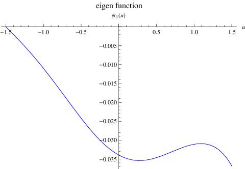
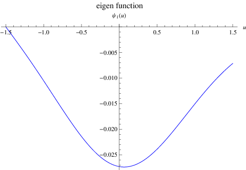
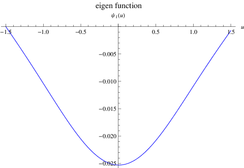
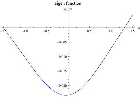
To illustrate this, let us take the example of $u_{0}=1.5,m=0$ . The plot of the eigenfunction using the eigenvalue $\lambda_{1}=-0.66$ ( which we got using AIM) and assuming $(\frac{d\psi_{1}}{du})_{u=-1.5}=-0.02$ has been shown in Fig. 7(a). Fig. 7(f) shows the correct eigenfunction obtained in the above way. The correct eigenvalue is $-0.385$ .

References

[1] J. L. Lagrange, Oeuvres, Vol. 1 (1760).
[2] J. Plateau, Recherches exp´rimentales et th´orique sur les ﬁgures d’´quilibre d’une masse liquide sans pesanteur, M´m Acad Roy Belgiuque 29 (1849).
[3] C. Isenberg, The science of soap films and soap bubbles, Dover Publications, N.Y., USA (1992).
[4] R. Osserman, A survey of minimal surfaces, Dover Publications, N. Y., USA (1986).
[5] L. Durand, Stability and oscillations of a soap film: An analytic treatment, Am. J. Phys, 49, 334 (1981).
[6] M. Ito and T. Sato, In situ observation of a soap-film catenoid- a simple educational physics experiment , Eur.J.Phys.31,357-365 (2010).
[7] M. Ben Amar, P.P. da Silva, N. Limodin, A. Langlois, M. Brazovskaia, C. Even, I.V. Chikina and P. Pieranski, Stability and vibrations of catenoid-shaped smectic films, Eur. Phys. J. B 3, 197 (1998).
[8] H. Goldstein, C. Poole and J. Safko, Classical Mechanics, Pearson Education, India (2009)
[9] Michael Beeson, Notes on Minimal Surfaces,
http://www.michaelbeeson.com/research/papers/IntroMinimal.pdf
[10] Lecture notes by H.Kuiper (Arizona State University), Sturm-Liouville problems, http://math.la.asu.edu/~kuiper/462files/SturmLiouville.pdf
[11] P. Dennery and A. Krzywicki, Mathematics for Physicists, Dover Publications, New York, USA (1996).
[12] H. Ciftci, R. L. Hall and N. Saad, Asymptotic iteration method for eigenvalue problems, J. Phys. A Math. Gen. 36 11807.
[13] H. T. Cho, A. S. Cornell, J. Doukas,and Wade Naylor, Black hole quasinormal modes using the asymptotic iteration method , Class.Quant.Grav. 27,155004 (2010).