Search for solar axions in XMASS, a large liquid-xenon detector
Abstract
XMASS, a low-background, large liquid-xenon detector, was used to search for solar axions that would be produced by bremsstrahlung and Compton effects in the Sun. With an exposure of 5.6 ton days of liquid xenon, the model-independent limit on the coupling for mass 1 keV is (90% C.L.), which is a factor of two stronger than the existing experimental limit. The bounds on the axion masses for the DFSZ and KSVZ axion models are 1.9 and 250 eV, respectively. In the mass range of 10–40 keV, this study produced the most stringent limit, which is better than that previously derived from astrophysical arguments regarding the Sun to date.
Keywords:
Axion, Sun, xenon1 Introduction
The axion is a hypothetical particle invented for solving the problem in strong interactions [1]. As the initial Peccei–Quinn–Weinberg–Wilczek model of axions is directly tied to the electroweak symmetry-breaking scale, an experimental search was relatively easy and the model was ruled out early. However, invisible axion models such as DFSZ [2] and KSVZ [3], whose symmetry-breaking scale is separated from the electroweak scale, are still viable. The DFSZ axions have direct couplings to leptons whereas the KSVZ axions (hadronic axions) do not have tree-level couplings to leptons. In these models, the mass of axions is
where , , and are the axion decay constant [4], the pion decay constant, and pion mass, respectively, and is the quark mass ratio.
At present, the search for axions as well as axion-like particles (ALPs) focuses on couplings to photons , nucleons and electrons . There are three types of searches: (1) laboratory-based experiments in which sources and detectors are prepared, (2) astrophysical investigations that examine any significant deviations in the properties of stars from theoretical predictions due to extra emission of energy, and (3) using laboratory detectors to look for axion signals from the Sun or cosmological relics. Experiments searching for axions have so far produced null results, but sensitivities continue to improve.
In experimental searches that utilize , a series of experiments using strong magnets [5, 6, 7] successfully improved sensitivities by increasing the magnetic field strength and the conversion length. The suggestion [8] to use Bragg scattering to improve sensitivity for solar axions in crystalline detectors was used in [9, 10, 11, 12]. Another way to enhance sensitivity is to exploit resonant absorption on nuclei [13]. To date, several experimental results are obtained in this scheme [14, 15, 16, 17, 18, 19, 20, 21, 22, 24, 23]. Significant improvement can be achieved if the signals can be read out efficiently. On the other hand, an efficient experimental search with has not been performed. A pioneering experiment used a Ge detector (710 g) [25] and a recent search used a Si(Li) detector (1.3 g) to search for signals from axions generated by the bremsstrahlung and Compton effect via the axioelectric effect [26].
The choice of target material strongly affects the reach of a solar axion experiment using axion coupling to electrons. Liquid Xe is both dense and has a high atomic numbers [27]. The XMASS detector, which uses 835 kg of liquid xenon in its sensitive volume, is suitable for this purpose. Its low energy threshold (0.3 keV) is also useful as the predicted energy spectrum is very soft and has a peak at less than 1 keV for light axions. Its low background (a few keV-1kg-1day-1) makes it particularly useful when searching for solar axions.
2 Expected Signal
The signals we searched for are produced by the Compton scattering of photons on electrons and the bremsstrahlung of axions from electrons in the Sun. The expected fluxes and spectra are derived as follows.
The solar axion flux produced by Compton scattering was calculated in [28, 29]. The axion differential flux is expressed as
| (1) |
where is the total energy of the axions, is the average distance between the Sun and the Earth, is the radius of the Sun, is the blackbody spectrum of photons, is the cross section for the Compton effect, and is the electron density at the radius . Since and is assumed to be much smaller than , the differential cross section is approximately a product of , and the total cross section [29] is expressed as
| (2) |
where is the fine structure constant, is the electron mass, is the axion’s coupling to electrons [4] which is in the DFSZ axion model [26], and is the velocity of the outgoing massive axion. is the ratio of the two Higgs vacuum expectation values of the model [4].
The energy spectrum of solar axions produced by the bremsstrahlung effect was calculated in [28, 30]. The differential energy spectrum is
| (3) |
where is the velocity of the electrons, is the energy spectrum of the electrons, is the cross section for the bremsstrahlung effect, and is the atom density at radius . The cross section is calculated by considering the energy conservation of the electron and axion system [30].
The temperature, electron density, and atomic density are given by the standard solar model BP05(OP) [31]. Figure 1 in Ref. [26] shows the energy spectra for various masses of axions. The bremsstrahlung component dominates below 10 keV, whereas the Compton contribution dominates at higher energy.
The expected energy spectrum to be observed with a detector is
| (4) |
where is the cross section for the axioelectric effect [32]. For the cross section, the expression of Eq. (3) in Ref. [26] is used for
| (5) |
where is the photoelectric cross section of the detector medium for gamma rays with energy . The photoelectric cross section is available in Ref. [33, 34]. The predicted energy spectra for a xenon target for various axion masses are shown in Fig. 1.
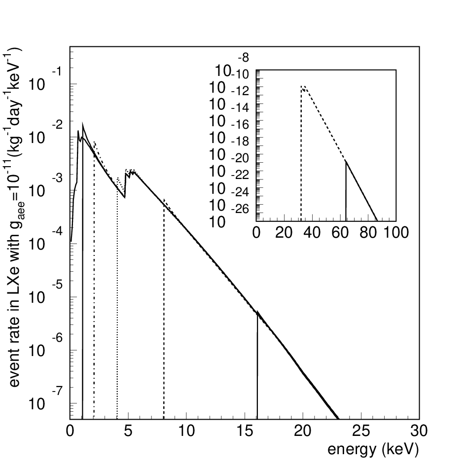
The predicted energy spectra calculated above are used to generate Monte Carlo simulation samples. Axion signal samples can be simulated by injecting gamma rays whose energy is the same as the total energy of the incoming axions. This is because (1) there is a relationship between the cross section of the axioelectric effect and the photoelectric effect as in Eq. (5), (2) the photoelectric effect is dominant in this energy range (100 keV), and (3) the process after the axioelectric effect is exactly the same as that for the photoelectric effect. In the simulation, we considered the nonlinearity of the scintillation yield for gamma rays, the optical processes of the scintillation photons in the detector, the photoelectron distributions and discrimination threshold of photomultipliers, and the trigger conditions of the data acquisition system. The detailed description of the simulation and efficiencies were previously reported [36, 35]. After taking into account the reduction efficiency described in the next section, the expected energy spectra for various masses of axions are obtained.
3 The Data
The XMASS detector is a large liquid-xenon detector located underground (3000 m water equivalent) at the Kamioka Observatory, Japan. It contains an 835-kg liquid-xenon target with a surface of a pentakis-dodecahedron that is tiled with inward looking photomultiplier tubes (PMT), 630 of which have hexagonal and 12 have round photocathodes. The PMTs (R-10789, Hamamatsu) are specially developed for this low-background detector. The photoelectron yield at the center of the detector is evaluated at 14.7 photoelectrons (p.e.)/keV using an internal 57Co source. The positional dependence (maximum 15%) of the photoelectron yield caused by the angular acceptance of PMTs and absorption of scintillation light are taken into account in the Monte Carlo simulations. Data acquisition is triggered if four or more PMTs have more than 0.2 p.e. within 200 ns. The trigger efficiency around the trigger threshold was examined by LEDs placed at the detector wall. The observed behavior was well reproduced by the Monte Carlo simulations. Signals from each PMT are fed into charge ADCs and TDCs whose resolution is around 0.05 p.e. and 0.4 ns, respectively. The liquid-xenon detector is surrounded by a water Cherenkov veto counter, which is 10.5 m in height and 10 m in diameter. It is equipped with 72 20-inch PMTs whose signals are fed into the ADCs and TDCs. Data acquisition is triggered if eight or more 20-inch PMTs have hits. The detector is described in detail in Ref. [36].
The data set used in the solar axion search experiments covers February 21–27, 2012. A sequence of standard data reduction is applied to remove events caused by afterpulses and electronic ringing. The standard reduction consists of a series of cuts: (1) the event is triggered only by the liquid-xenon detector; (2) the time difference to the previous event is more than 10 ms; (3) the root mean square of the hit timing is less than 100 ns and is used to reject events caused by afterpulses of PMTs due to bright events; and (4) the number of PMT hits in the first 20 ns divided by the total number of hits is less than 0.6 for events in which the number of photoelectrons is less than 200. The fourth cut was applied to remove Cherenkov events originated from 40K in photocathodes (Cherenkov cut). The energy threshold of this analysis is low (0.3 keV) because of our exceptional photoelectron yield, which is the largest among current low-background detectors. A more detailed description of the reduction can be found in Ref. [35].
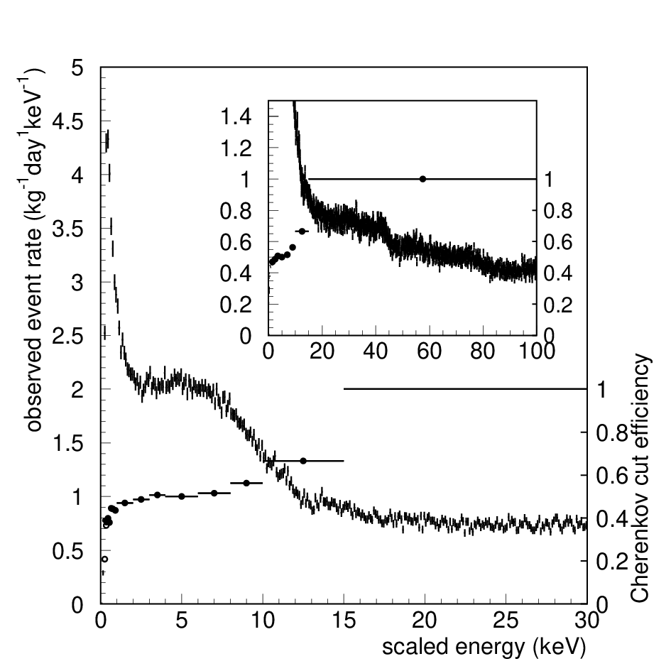
Figure 2 shows the observed energy spectra. The total livetime is 6.7 days after considering the dead time caused by the cut (2). The effect of trigger cut (1) is visible below 0.4 keV as shown in Fig. 3 in Ref. [35] and is considered in our Monte Carlo simulations. The same samples show that the cut (3) has negligible effect on the signals. The signal efficiency due to the Cherenkov cut, which is drawn in the same figure, was conservatively evaluated using low-energy gamma-ray sources such as 55Fe and 241Am sources at various positions. Because the efficiency weakly depends on the radial position of the events and gradually decreases outward, the efficiency adopted in the analysis was mostly evaluated at a radius of 40 cm where 93% of the mass was contained inside. The Monte Carlo samples were compared with the observed energy spectra after weighting this efficiency.
4 Limit on
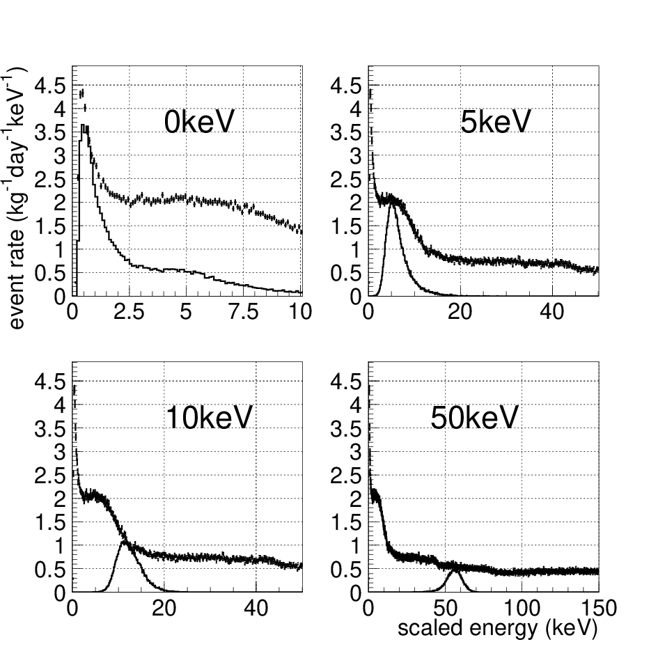
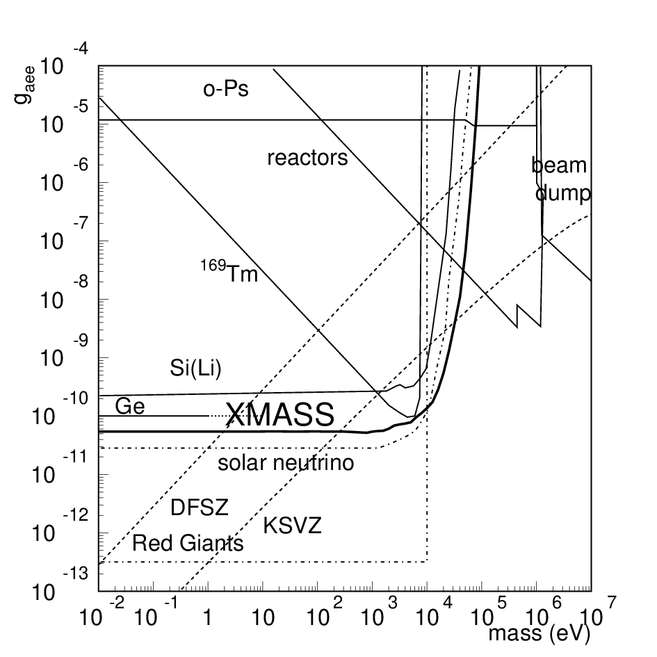
The observed spectra do not have any prominent features to identify axion signals with respect to the background. Instead, strong constraints on can be obtained from the observed event rate in the relevant energy range. In order to set a conservative upper limit on the axion-electron coupling constant , the coupling is adjusted until the expected event rate in XMASS does not exceed the one observed in any energy bin above 0.3 keV. Figure 3 shows the expected energy spectra with the coupling constants obtained by the procedure above. Figure 4 shows the summary of the bounds of . For small axion masses, a value of is obtained. This is the best direct experimental limit to date and is close to that derived from astrophysical considerations based on measured solar neutrino fluxes: [37]. For axion masses 10 keV the energetics in the Sun are no longer sufficient to effectively produce such axions. A systematic uncertainty inherent to our method of comparing bin contents arises from the specific choice of binning. This and systematic uncertainties for energy scale including energy threshold, Cherenkov cut efficiency, and energy resolution are evaluated to be 2%, 1%, 2%, and 1%, respectively. The total systematic error, 3%, is obtained by summing these contributions in quadrature, and the limit in Fig. 4 (90% C.L.) takes this error into account.
The calculated limit depends on the interaction processes considered in our detector as well as the processes considered for solar axion production in the Sun. Processes such as the inverse Primakoff effect and nuclear absorption on the detection side, and the Primakoff effect and nuclear deexcitation on the production side can be neglected because the constraints on and are tight. A possible additional contribution caused by on the detection side is the inverse Compton effect. This can be neglected because of its small cross section [38]. On the production side, there are other known contributions such as electron-electron bremsstrahlung [39] and the axio-recombination effect [40]. However, the expected fluxes for these processes are only known in the limit of massless axions. For this reason and in order to directly compare our results with the most relevant previously published ones we restrict the production processes we consider to the electron-nuclei bremsstrahlung and the Compton effect. As omitting production mechanisms lowers the flux estimate, all the limits thus derived will have to be considered conservative.
The nature of the events surviving the analysis cuts is also of interest. According to our study on these events, most of them originate on the inner surface of the detector [41]. These events are attributed to radioactive contamination in the aluminum seal of the PMT entrance windows, 14C decays in the GORE-TEX® sheets between the PMTs and the copper support structure, and light leaking from gaps in between the triangular elements of this support structure.
5 Conclusion
In summary, solar axions produced through axion-electron coupling were searched for in XMASS, a large liquid-xenon detector. The energy threshold is low (0.3 keV) because of our exceptional photoelectron yield, which is the largest among current low-background detectors. As our observed spectrum does not show any indications of axion signals, we derive constraints on the coupling. Our limit on for axions with mass much smaller than 1 keV is . The bounds on the axion masses for the DFSZ and KSVZ axion models are 1.9 and 250 eV, respectively. For axion masses between 10 and 40 keV, our new limits are the most stringent that are currently available.
Acknowledgements
We gratefully acknowledge the cooperation of Kamioka Mining and Smelting Company. This work was supported by the Japanese Ministry of Education, Culture, Sports, Science and Technology, Grant-in-Aid for Scientific Research, and partially by the National Research Foundation of Korea Grant funded by the Korean Government (NRF-2011-220-C00006). We thank J. Redondo for useful discussion.
References
- [1] R. D. Peccei and H. R. Quinn, Phys. Rev. Lett 38 (1977) 1440; R. D. Peccei and H. R. Quinn, Phys. Rev. D 16 (1977) 1791; S. Weinberg, Phys. Rev. Lett. 40 (1978) 223; F. Wilczek, Phys. Rev. Lett. 40 (1978) 279.
- [2] M. Dine, W. Fischler, M. Srednicki, Phys. Lett B 104 (1981) 199; A. R. Zhitnitsky, Sov. J. Nucl. Phys. 31 (1980) 260 [Yad. Fiz. 31 (1980) 497].
- [3] J. E. Kim, Phys. Rev. Lett. 43 (1979) 103; M. A. Shifman, A. I. Vainshtein and V. I. Zakharov, Nucl. Phys. B 166 (1980) 493.
- [4] G. G. Raffelt, Lect. Notes Phys. 741 (2008) 51.
- [5] D. M. Lazarus et al., Phys. Rev. Lett. 69 (1992) 2333.
- [6] S. Moriyama et al., Phys. Lett B 434 (1998) 147; Y. Inoue et al., Phys. Lett. B 536 (2002) 18; Y. Inoue et al., Phys. Lett. B 668 (2008) 93.
- [7] S. Andriamonje et al., JCAP 0704 (2007) 010; E. Arik et al., JCAP 0902 (2009) 008; S. Aune et al., Phys. Rev. Lett. 107 (2011) 261302.
- [8] E. A. Paschos and K, Zioutas, Phys. Lett. B 323 (1994) 367.
- [9] F. T. Avignone et al., Phys. Rev. Lett. 81 (1998) 5068.
- [10] R. Bernabei et al., Phys. Lett B 515 (2001) 6.
- [11] A. Morales et al., Astropart. Phys. 16 (2002) 325.
- [12] Z. Ahmed et al., Phys. Rev. Lett 103 (2009) 141802.
- [13] S. Moriyama, Phys. Rev. Lett. 75 (1995) 3222.
- [14] M. Krcmar et al., Phys. Lett. B 442 (1998) 38.
- [15] M. Krcmar, Z. Krecak, A. Ljubicic, M. Stipcevic, and D. A. Bradley, Phys, Rev. D 64 (2001) 115016.
- [16] K. Jakovcic, Z. Krecak, M. Krcmar, A. Ljubicic, Rad. Phys. and Chem., 71 (2004) 793.
- [17] A. V. Derbin et al., JETP Lett. 85 (2007) 12.
- [18] T. Namba, Phys. Lett. B 645 (2007) 398.
- [19] A. V. Derbin et al., Bull. Rus. Acad. Sci. Phys. 71 (2007) 832.
- [20] P. Belli et al., Nucl. Phys. A, 806 (2008) 388.
- [21] A. V. Derbin et al., Eur. Phys. J. C 62 (2009) 755.
- [22] A. V. Derbin et al., Phys. Atom. Nuclei 74 (2011) 596.
- [23] G. Bellini et al., Phys. Rev. D 85 (2012) 092003.
- [24] P. Belli et al., Phys. Lett. B 711 (2012) 41.
- [25] F. T. Avignone, R. L. Brodzinski, S. Dimopoulos, G. D. Starkman, A. K. Drukier, D. N. Spergel, G. Gelmini, B. W. Lynn, Phys. Rev. D. 35 (1987) 2752.
- [26] A. V. Derbin et al., JETP Lett. 95 (2012) 379, arXiv:1206.4142v2.
- [27] F. T. Avignone III, R. J. Creswick, S. Nussinov, Phys. Lett. B 681 (2009) 122.
- [28] A. V. Derbin, A. S. Kayunov, V. V. Muratova, D. A. Semenov, and E. V. Unzhakov, Phys. Rev. D 83 (2011) 023505.
- [29] M. Pospelov, A. Ritz, and M. Voloshin, Phys. Rev. D 78 (2008) 115012.
- [30] A. R. Zhitnitskiĭ and Y. I. Skovpen’, Sov. J. Nucl. Phys. 29 (1979) 513.
- [31] J. N. Bahcall, A. M. Serelli, and S. Babu, Astrophys. J. 621 (2005) L85.
- [32] A. Derevianko, V. A. Dzuba, V. V. Flambaum, M. Pospelov, Phys. Rev. D 82 (2010) 065006.
- [33] M. J. Berger, J. H. Hubbel, S. M. Seltzer, et al., XCOM: Photon Cross Sections Database http://www.nist.gov/pml/data/xcom/index.cfm
- [34] WM. J. Veigele, Atomic Data Table 5 (1973) 51.
- [35] K. Abe et al. (XMASS collaboration), Phys. Lett B 719 (2013) 78.
- [36] K. Abe et al. (XMASS collaboration), Nucl. Instr. Meth. A 716 (2013) 78.
- [37] P. Gondolo and G. G. Raffelt, Phys. Rev. D 79, 107301 (2009).
- [38] R. Bernabei et al., Int. J. Mod. Phys. A 21 (2006) 1445.
- [39] G. G. Raffelt, Phys. Rev. D 33 (1986) 897.
- [40] S. Dimopoulos, J. Frieman, B. W. Lynn, and G. D. Starkman, Phys. Lett. B 179 (1986) 223.
- [41] Y. Suzuki for the XMASS collaboration, Proceedings of the International Workshop on the Identification of Dark Matter, Chicago, USA, 23-27 July, 2012.