Classical Model Predictive Control
of a Permanent Magnet Synchronous Motor

In a fist step the machine model is linearized. This will result in a linear-quadratic optimization problem with linear constraints, a very common problem in optimal control systems [13] that is also simpler to solve in real-time. Assuming that the rotor speed does not change too much over the optimization horizon $T$,

$\displaystyle\frac{d}{dt}\omega_{M}(t)$

$\displaystyle\approx 0\;\;\Rightarrow\omega_{M}(t)=\textnormal{const. }\;\;\forall t\in[0,T],$

(1)

the PMSM model and the voltage equations become linear. The assumption is justified if the current control loop is faster than the speed control loop. The electrical subsystem of the machine, consisting of the quadrature and direct currents $i_{q}$ and $i_{d}$ (peak values), is given as

	$\displaystyle L_{d}\frac{\textnormal{d}}{\textnormal{dt}}i_{d}$	$\displaystyle=-Ri_{d}+n_{p}\omega_{M}L_{q}i_{q}+u_{d},$		(2)
	$\displaystyle L_{q}\frac{\textnormal{d}}{\textnormal{dt}}i_{q}$	$\displaystyle=-Ri_{q}-n_{p}\omega_{M}L_{d}i_{d}-n_{p}\omega_{M}K+u_{q},$		(3)
	$\displaystyle\tau_{M}$	$\displaystyle=\frac{3}{2}n_{p}Ki_{q}.$		(4)

The nomenclature is shown in table II in the appendix. It is noted that the reluctance torque $\tau_{M}^{R}=\frac{3}{2}n_{p}(L_{d}-L_{q})i_{d}i_{q}$ is neglected, as this term is very small compared to the electromagnetic torque in surface-mounted PMSMs or in machines with small saliency. Furthermore, it would render the model nonlinear, requiring nonlinear optimization methods [14].

The formulation of a suitable cost functional is a key point in predictive control, as it is the only tuning possibility of the control scheme. The optimization is aiming at minimizing the control error for good dynamical performance as well as machine losses for better efficiency. Both goals are included in the cost functional. By choosing the cost functional and weights well, it is possible to find a good trade-off between both goals during transients, and eventually to fulfill both goals in steady-state. The cost functional for the predictive torque controller is

$\displaystyle J=\int_{0}^{T}\left(P_{ctrl}(t)+W_{L}\cdot P_{loss}(t)\right)dt+T\cdot P_{ctrl}(T)$

(5)

which trades off the squared control error from the constant torque reference $\tau_{M}^{*}$

$\displaystyle P_{ctrl}(t)=(\tau_{M}-\tau_{M}^{*})^{2}$

(6)

with machine losses

	$\displaystyle P_{loss}(t)$	$\displaystyle=\frac{3}{2}R(i_{d}^{2}+i_{q}^{2})+\frac{3}{2}n_{p}\omega_{M}k_{Fe}(\Psi_{d}^{2}+\Psi_{q}^{2})$
	$\displaystyle=$	$\displaystyle\frac{3}{2}R(i_{d}^{2}+i_{q}^{2})+\frac{3}{2}n_{p}\omega_{M}k_{Fe}((L_{d}i_{d}+K)^{2}+(L_{q}i_{q})^{2}).$		(7)

The first term in $P_{loss}$ represents copper losses, and the second term represents the iron losses consisting of hysteresis losses. The last term in (5) is the end-weight of the control error, it serves to improve convergence within finite time, especially when constraints are active. Its effect is shown in the results section. Eddy current losses are negligible on the tested machines, however, they could be included using the model presented in [15]. The machine losses can be reduced by field-weakening, where a trade-off between copper and iron losses is found [16]. Imposing a negative direct current $i_{d}$, the flux magnitude in the stator is reduced while the copper losses increase. As the iron loss constant $k_{Fe}$ is not part of standard motor parameters, it has to be determined experimentally [17]. The iron losses are quite considerable, for instance, the applied $2.64$ kW machine has about $43$ W copper losses and $200$ W iron losses in rated operation, therefore the parameter $k_{Fe}$ can be determined using only standard equipment. Inverter losses remain undiscussed as the switching frequency is arbitrary fixed.

There are two tuning parameters, $W_{L}$ and $T$. The weight $W_{L}$ was set $0.05$, the value was determined heuristically. The optimization horizon is set $T=2$ ms such that the cost functional includes the complete setpoint change. It is important that the optimization horizon is high enough, otherwise the open-loop and closed-loop trajectories differ and the behavior is strongly suboptimal. This is illustrated in Fig. 1 (left). The open-loop trajectory, a continuous trajectory optimal with respect to $J$, is generated and a first part is applied to the system. At the next sampling step (indicated by a circle), a new open-loop trajectory is generated and again its first part is applied to the system. The resulting closed-loop trajectory, which is the sequence of the discrete points at each sampling interval, differs significantly from the open-loop trajectories, especially if the horizon is too small. Then, the closed-loop trajectories simply do not fit the cost functional anymore and are suboptimal. For a horizon higher than required for the setpoint change, as shown in Fig. 1 (right), the difference between open- and closed-loop trajectories becomes smaller. Ideally the points should be superposed with the continuous open-loop trajectories, then, the closed-loop trajectories can be assumed optimal regarding the open-loop cost functional $J$.

The most important nonlinearities of a PMSM, in terms of control, are the voltage and current limitations. The current constraints prevent overheating of the machine, and the voltage is limited by the maximum output voltage of the voltage source inverter. The voltage constraints limit rotor speed as well as current dynamics in high-speed operation. Both constraints are approximated by affine equations, in order to be computationally efficiently treated.

The current range for the direct current $i_{d}$ is limited to $i_{d}^{min}\leq i_{d}\leq 0$. Only negative values of $i_{d}$ are desirable, as they improve power efficiency and reduce the induced voltage by weakening the flux magnitude in the stator [16, 5]. The lowest value $i_{d}^{min}$ is the optimum value at rated speed ($\frac{\partial}{\partial i_{d}}P_{loss}=0$) and is given as

$\displaystyle i_{d}^{min}=-\frac{L_{d}K}{L_{d}^{2}+R(n_{p}\omega_{MN}k_{Fe})^{-1}},$

(8)

which is independent of quadrature current $i_{q}$ if the reluctance torque and the saliency are neglected, what is acceptable for surface-mounted PMSMs [15]. The value is doubled to enable further field-weakening to improve dynamics in high speed, an effect described in the results section. For the quadrature current $i_{q}$, the largest possible range of values should be available. The resulting linear constraints, shown in Fig. 2, almost completely fill the current region of interest. A representation with affine inequality constraints is thus acceptable.

The approximation of the voltage constraints is a bit more difficult. The $q$-axis should not be restricted, as the induced voltage is aligned to it and is the largest value that will appear. A steady-state analysis of the system equations (2), (3) shows that a rectangular voltage area results

	$\displaystyle Ri_{d}^{min}\mbox{-}n_{p}L_{q}\omega_{M}^{max}i_{q}^{max}$	$\displaystyle\leq u_{d}\leq n_{p}L_{q}\omega_{M}^{max}i_{q}^{max},$		(9)
	$\displaystyle\mbox{-}Ri_{q}^{max}\mbox{+}n_{p}L_{d}\omega_{M}^{max}i_{d}^{min}\mbox{-}n_{p}K\omega_{M}^{max}$	$\displaystyle\leq u_{q}\leq Ri_{q}^{max}\mbox{+}n_{p}K\omega_{M}^{max}.$		(10)

This rectangle (dark grey on Fig. 2) is expanded such that the outer circle of the voltage limitation is hit (light grey on Fig. 2). During dynamical transients, the voltage vector points to one of the outer corners, subsequently touching the outer limiting circle. Therefore, a linear approximation of the voltage limits as a rectangle by the presented method, as shown on Fig. 2, does not limit the steady-state operational range and only marginally affects dynamics. A less restrictive method is presented in [6], where a time-varying constraint in form of a hexagon in stator frame is proposed. The limiting circle can be expanded to a hexagon by using overmodulation techniques [18]. While this is possible too with the underlying predictive control algorithm, the method in the ($d,q$)-frame is chosen for simplicity and to prevent possible current ripples.

The trajectory generation algorithm presented in [11], a development related to flatness-based methods [10], is chosen. It can optimize a quadratical cost function with linear constraints. As major differences to standard algorithms, it is applying a continuous parameterization instead discretization, and the computationally efficient linear programming solver is used instead of quadratic programming or iterative gradient search. Even though LP is used, it is still quadratic optimization; the unconstrained solution to the quadratic cost is calculated first, then, constraints are included with the LP solver.

The trajectories for the current are defined as degree $n$ power series with undetermined coefficients $\alpha_{ij}$,

$\displaystyle i_{d}(t)=\sum_{k=0}^{n}\alpha_{dk}\ \frac{t^{k}}{T^{k}},\;\;\;\;i_{q}(t)=\sum_{k=0}^{n}\alpha_{qk}\ \frac{t^{k}}{T^{k}},\;\;\;\;t\in[0,T].$

(11)

This definition reduces the dimensionality of the generated trajectories rather than their length and is referred to as Ritz parameterization [13]. It is an alternative parameterization to the typical Euler discretization. The first coefficients $\alpha_{d0}$ and $\alpha_{q0}$ are the initial conditions, and the remaining $6$ coefficients are determined by optimization. A high prediction horizon is obtained for a relatively small number of parameters. Due to the analyzed computational limitations, $n=3$ is chosen as polynomial degree. Fig. 3 illustrates the computational advantage, with $3$ parameters at $8$ kHz sampling rate, using a discrete description, the prediction horizon is $0.375$ ms, but with a degree $3$ polynomial, a well-conditioned setpoint change can be described over the desired prediction horizon of $2$ ms. A more complex trajectory may not be expected for the underlying application.

The corresponding voltages $\bm{u}_{dq}(t)$ are computed by algebraic differentiation of (11) and by solving for the model equations (2) and (3), this is also called the flatness-based approach [20]. This way, the voltages do not need to be represented by additional parameters, and equality constraints are avoided in the optimization. The variables $\bm{i}_{dq}$, $\frac{\textnormal{d}}{\textnormal{dt}}\bm{i}_{dq}$ and $\bm{u}_{dq}$ are substituted in the cost functional $J$ (5) by the found functionals.

The cost functional $J$ is then a quadratic function of the unknown parameters $\bm{\alpha}$ and of the parameters which were assumed constant, namely the motor parameters, the measured currents, the speed $\omega_{M}$ and the torque reference $\tau_{M}^{*}$. Defining the vector of undetermined coefficients as $\bm{\alpha}=(\alpha_{d1},\alpha_{d2},\alpha_{d3},\alpha_{q1},\alpha_{q2},\alpha_{q3})^{T}$, it is written as

$\displaystyle J=\bm{\alpha}^{T}\bm{Q}\bm{\alpha}+\bm{q}^{T}\bm{\alpha}+q_{0}.$

(12)

Because of the parameterization with a polynomial basis, convexity must be discussed [10], in (5) the weight matrix was $\mathbb{R}^{2x2}$ whereas now it is extended to $\bm{Q}\in\mathbb{R}^{6x6}$. Convexity guarantees the existence of a unique global minimum, and convergence of the optimization algorithm in finite time. The proof that convexity is maintained with this transformation is given in [11]. Graphically, for a simple example with two parameters, $J$ can be represented as in Fig. 4 (left).

The inequality constraints are also parameterized with the polynomial. Exact parameterization requires linear matrix inequality (LMI) methods, which are however too involved for this application. A simpler way is to sample the trajectories for $\bm{i}_{dq}(t)$ and $\bm{u}_{dq}(t)$ at an interval $\frac{T}{n}$. In [11] it is proven that if an additional interlay is added, the transformation guarantees maintenance of the original constraints. For instance, a constraint $i_{d}(t)\leq 0\forall t\in[0,T]$ is parameterized as

	$\displaystyle i_{d}(0)$	$\displaystyle\leq 0,$		(13)
	$\displaystyle i_{d}(k\frac{T}{n})-\Delta i_{d}(0)$	$\displaystyle\leq 0\;k=1..3,$		(14)

where $\Delta=0.064$ is the respective interlay constant for $n=3$ (see [11]). The first constraint on the initial condition does not need to be included, and the remaining $3$ conditions are affine functions of $\bm{\alpha}$, but not of $t$, such that they can directly be included in linear-quadratic optimization in the parameter space $\bm{\alpha}$.

As $J$ is convex, the unconstrained global optimum $\bm{\alpha}_{0}^{*}$ is found algebraically by solving first-order necessary conditions,

$\displaystyle\bm{\alpha}_{0}^{*}=-\frac{1}{2}\bm{Q}^{-1}\bm{q}.$

(15)

Then, by an affine coordinate transformation

$\displaystyle\bm{\beta}=\bm{A}(\bm{\alpha}-\bm{\alpha}_{0}^{*}),$

(16)

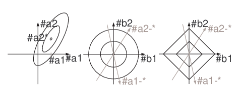
the problem can be reformulated as least-distance problem, i.e. a quadratical cost describing the distance to the unconstrained optimum. The linear transformation includes a shift of the origin of the coordinates, a coordinate rotation as well as a coordinate scaling, and is found with

$\displaystyle\bm{A}^{T}\bm{A}=\bm{Q},$

(17)

which can be solved with the Cholesky decomposition $\bm{A}^{T}=\textnormal{cholesky}(\bm{Q}^{T})$. As result, the cost functional looks much simpler and reduces to a sum of squares

$\displaystyle J=\bm{\beta}^{T}\bm{\beta},$

(18)

and can be represented as in Fig. 4 (middle). The unconstrained optimum is thereby $\bm{\beta}_{0}^{*}=\bm{0}$. This constrained least-distance problem is already simpler to solve than the original problem. In the next step, the least-distance problem is linearized around the unconstrained optimum, see Fig. 4 (right). The squares in the cost function are replaced by absolute values

$\displaystyle J=\bm{\beta}^{T}\bm{\beta}=\sum_{i}\beta_{i}^{2}\approx\sum_{i}|\beta_{i}|=J^{\prime}.$

(19)

In the LP standard form, furthermore, only positive parameters are possible, therefore the variables are replaced by $\beta_{i}=\beta_{ip}-\beta_{in}$, with $\beta_{ip},\beta_{in}\geq 0$. The absolute value can then be replaced by $|\beta_{i}|=\beta_{ip}+\beta_{in}$. Equivalence is guaranteed by minimizing the (positive) sum, such that at least one variable of each pair $(\beta_{ip},\beta_{in})$ will be zero [13]. The linearization of the cost function inherits a large error in the value of $J$, but the values of the coefficients $\beta$ are not affected that much: the least-distance problem is not so much different in the linear form as it would have been in the quadratical form. Furthermore, see that a difference only appears if a constraint is active, the unconstrained optimum is the same. Suboptimality is evaluated in the results section based on numerical simulations. The linear constraints on $\bm{\alpha}$ are as well transformed directly with (16). Therefore, after all the transformations, the problem is available in standard form for linear programming, and a simplex solver [19] can be run. The optimal solution $\bm{\beta}^{*}$ has to be retransformed to find the optimum in the original coordinates

$\displaystyle\bm{\alpha}^{*}=\bm{\alpha}_{0}+\bm{A}^{-1}\bm{\beta}^{*},$

(20)

which is used in (11) and the motor model to obtain the optimal trajectories for the currents and voltages.

All computations of the previous section are done using a computer algebra tool (Maplesoft Maple). The matrices for the LP solver are generated using the C code generation toolbox. The real-time software thus consists of a simplex tableau assignment, consisting of the initialization of one matrix and two vectors of floating-point variables, which is automatically generated code, a simplex LP solver from [19], and some post-processing. As the assignment is based on symbolic calculations, the motor parameters can be changed online. However, the majority of parameters is defined as constant, the compiler can then optimize code size as well as runtime of the initialization stage.

Alternatives to this procedure were evaluated. The direct use of a quadratic program is too slow, for instance, with $6$ parameters, $16$ (voltage) constraints and $20$ iterations it requires $730$ $\mu$s - if additionally current constraints were included, it would take even longer. If the problem is first transformed to least-distance, the number of iterations and the runtime reduce to about $50\%$.

Also online calculation of the trajectory generation algorithm instead of computer algebra generated code was analyzed. The matrix inversion with $6$ parameters takes $2.5$ $\mu$s and the cholesky decomposition $40$ $\mu$s. Additionally this requires the use of a scientific mathematics library.

The choice to use a computer algebra tool and automatic code generation turns out as the easiest way to implement and as well as computationally most efficient. The automatically generated code is copy-and-pasted to the real-time software, only a small LP solver like [19] has to be added. The chosen LP implementation, however, seems to be a somewhat slow implementation, runtime improvements are possible.

The control structure is shown in Fig. 5. A cascaded control structure is chosen as speed is assumed constant for trajectory generation. As the mechanical plant is generally only roughly known, this overlying speed controller is advantageous. Model-based control can be used for the electrical subsystem of the motor as the parameters are known, but for the mechanical part, any robust feedback controller can be chosen.

The trajectory generation scheme is embedded in a predictive controller and repeated at every sampling step to generate the optimal control input $\bm{u}_{dq}[k]$.

Additionally, for steady-state accuracy, a disturbance observer is necessary, for instance to compensate modeling errors of the induced voltage terms. Even though the induced voltage is modeled, variations in $K$ caused for instance by heating or identification errors cause an offset of the current $i_{q}$. The approach is to assume the disturbance as constant and calculate it directly based on the MPC model and past control inputs and current measurements [21]. The respective delays have to be accounted in the design.

First, measurement and control timing is analyzed. Two timing sequences are shown in Fig. 6 (a) and (b). The interrupt-based control system triggers an interrupt every $125$ $\mu$s (signal 3). At this instant, the applied voltage command (signal 2) is modulated in the power electronics. At the same instant, the A/D conversion of the current measurements (signal 1) is performed to avoid the impact of current ripples. It is seen that to calculate the command $u_{q}[k]$, only the current $i_{q}[k-1]$ is available. Furthermore, once the command $u_{q}[k]$ is calculated, it needs to wait until the next interrupt. This delay of one step is denoted computational delay and is accounted with a delay compensation technique. A prediction of one sampling step with the model, the current $i_{q}[k-1]$ as well as the previously commanded voltage $u_{q}[k-1]$ is applied to generate the delay-compensated current $i_{q}[k|k-1]$ as initial condition for the control law to compute $u_{q}[k]$, see [22]. Furthermore, see that the response to the commanded voltage $u_{q}[k]$ is $i_{q}[k+1]$ which is available one interrupt later, this is the plant delay and it is naturally included in the predictive controller by recalculating the trajectory at every sampling step. From the predicted trajectory, the applied voltage is $\bm{u}_{dq}[k]=\bm{u}_{dq}(0)$.

From the timing sequences, interesting insight into the computational demands of the algorithm is gained. The first part of the controller signal in Fig. 6 shows the calculation time for the simplex tableau initialization, it takes about $10\mu$s. Included in these calculations, which is automatically generated code resulting from symbolical calculations, is a calculation of the unconstrained optimum and the linearization of the problem. The second and biggest part of the controller signal is the runtime of the linear program [19]. At the beginning of Fig. 6 (a), where voltage and current are both zero, it is only about $20\mu$s, but to calculate the voltage step at $2000$ rpm shown in Fig. 6 (b), more iterations are involved as many constraints are active, and the computation time rises to almost $60\mu$s. The total time of the interrupt handling, latency, the simplex initialization, the LP solver and the post-processing sum up to almost $100\mu$s in the worst case, therefore up to $80\%$ of the available time is used.

References

- [2] P. Cortés, M. Kazmierkowski, R. Kennel, D. Quevedo and J. Rodriguez, Predictive control in power electronics and drives, IEEE Trans. Ind. Electron., Vol. 55, No. 2, pp. 4312–4324, 2008.
- [3] T. Geyer, G.A. Beccuti, G. Papafotiou and M. Morari, Model predictive direct torque control of permanent magnet synchronous motors, Energy Convers. Congress and Exp., pp. 199–206, 2010.
- [4] S. Bolognani, R. Kennel, S. Kuehl and G. Paccagnella, Speed and current model predictive control of an IPM synchronous motor drive, Proc. IEEE Int. Electric Machines and Drives Conf., pp. 1597–1602, 2011.
- [5] S. Bolognani, S. Bolognani, L. Peretti and M. Zigliotto, Combined speed and current model predictive control with inherent field-weakening features for PMSM drives, Proc. of the IEEE Med. Electrotechnical Conf., pp. 472–478, 2008.
- [6] S. Richter, S. Mariéthoz and M. Morari, High-speed online MPC based on a fast gradient method applied to power converter control, Proc. of the American Control Conf., pp. 4737–4743, 2010.
- [7] J.H. Lee, Model predictive control: Review of three decades of development, Int. J. Control, Automation and Systems, Vol. 9, No. 3, pp. 415–424, 2011.
- [8] M. Fliess and R. Marquez, Continuous-time linear predictive control and flatness: a module-theoretic setting with examples, Int. J. of Control, Vol. 73, No. 7, pp. 606–623, 2000.
- [9] V. Hagenmeyer and E. Delaleau, Continuous-time non-linear flatness-based predictive control: an exact feedforward linearization setting with an induction drive example, Int. J. of Control, Vol. 81, No. 10, pp. 1645–1663, 2008.
- [10] M. Guay and J.F. Forbes, Real-time dynamic optimization of controllable linear systems, J. of Guidance, Control and Dynamics, Vol. 29, No. 4, pp. 929–935, 2006.
- [11] J-F. Stumper and R. Kennel, Computationally efficient trajectory optimization for linear control systems with input and state constraints, Proc. of the American Control Conf., pp. 1904–1909, 2011.
- [12] J-F. Stumper, A. Dötinger, J. Jung and R. Kennel, Predictive control of a permanent magnet synchronous machine based on real-time dynamic optimization, Proc. Europ. Conf. on Power Electron. And Appl., paper 99, 2011.
- [13] D.A. Pierre, Optimization theory with applications. New York: Wiley, 1969.
- [14] E. Delaleau and A.M. Stanković, Flatness-based hierarchical control of the PM synchronous motor, Proc. of the American Control Conf., pp. 65–70, 2004.
- [15] C. Mademlis, J. Xypteras and N. Margaris, Loss minimization in surface permanent-magnet synchronous motor drives, IEEE Trans. Ind. Electron., Vol. 47, No. 1, pp. 115–122, 2000.
- [16] C. Cavallaro, A.O. Di Tommaso, R. Micelli, A. Raciti, G.R. Galluzzo and M. Trapanese, Efficiency enhancement of permanent-magnet synchronous motor drives by online loss minimization approaches, IEEE Trans. Ind. Electron., Vol. 52, No. 4, pp. 1153–1160, 2005.
- [17] N. Urasaki, T. Senjyu and K. Uezato, A novel calculation method for iron loss resistance suitable in modeling permanent-magnet synchronous motors, IEEE Trans. Energy Convers., Vol. 18, No. 1, pp. 41–47, 2003.
- [18] N.P. Quang and J.A. Dittrich, Vector control of three-phase AC machines: System development in the practice. Berlin: Springer Verlag, 2008.
- [19] W.H. Press, S.A. Teukolsky, W.T. Vetterling and B.P. Flannery, Numerical recipes in C: the art of scientific computing, 2nd ed., Ch. 10.8. Cambridge: Cambridge University Press, 1992.
- [20] H. Sira-Ramírez and S.K. Agrawal, Differentially flat systems, Ch. 8.2. New York: Marcel Dekker, 2004.
- [21] K.H. Kim and M.J. Youn, A simple and robust digital current control technique of a PM synchronous motor using time delay control approach, IEEE Trans. Power Electron., Vol. 16, No. 1, pp. 72–82, 2001.
- [22] H-T. Moon, H-S. Kim and M-J. Youn, A discrete-time predictive current control for PMSM, IEEE Trans. Power Electron., Vol. 18, No. 1, pp. 464–472, 2003.
- [23] N.A. Ameen, A.A. Naassani, R. Kennel, Design of a digital system dedicated for electrical drive applications, EPE J., Vol. 20, No. 4, pp. 37–44, 2010.
- [24] J.W. Choi and S.K. Sul, Generalized solution of minimum time current control in three-phase balanced systems, IEEE Trans. Power Electron., Vol. 45, No. 5, pp. 738–744, 1998.
Appendix: Motor Parameters