Degree of mobility for metrics of lorentzian signature and parallel (0,2)-tensor fields on cone manifolds

Aleksandra Fedorova and Vladimir S. Matveev Address: Mathematisches Institut, Friedrich-Schiller Universität Jena
07737 Jena, Germany Email address: vladimir.matveev@uni-jena.de

Abstract.

Degree of mobility of a (pseudo-Riemannian) metric is the dimension of the space of metrics geodesically equivalent to it. We describe all possible values of the degree of mobility on a simply connected n-dimensional manifold of lorentz signature. As an application we calculate all possible differences between the dimension of the projective and the isometry groups. One of the main new technical results in the proof is the description of all parallel symmetric $(0,2)$ -tensor fields on cone manifolds of signature $(n-1,2)$ .

1. Introduction.

1.1. Main definitions and results.

Let $(M^{n},g)$ be a connected Riemannian (= $g$ is positively definite) or pseudo-Riemannian manifold of dimension $n\geq 3$ . Within the whole paper we assume that all objects are $C^{\infty}$ -smooth. We say that a metric $\bar{g}$ on $M^{n}$ is geodesically equivalent to $g$ , if every geodesic of $g$ is a (reparametrized) geodesic of $\bar{g}$ . We say that they are affinely equivalent, if their Levi-Civita connections coincide.

As we recall in Section 2.1, the set of metrics geodesically equivalent to a given one (say, $g$ ) is in one-to-one correspondence with nondegenerate solutions of the equation (10). Since the equation (10) is linear, the space of its solutions is a linear vector space. Its dimension is called the degree of mobility of $g$ and will be denoted by $D(g)$ . Locally, the degree of mobility of $g$ coincides with the dimension of the set (equipped by its natural topology) of metrics geodesically equivalent to $g$ .

The degree of mobility is at least one (since $\operatorname{const}\cdot g$ is always geodesically equivalent to $g$ ) and is at most $\tfrac{(n+1)(n+2)}{2}$ , which is the degree of mobility of simply-connected spaces of constant sectional curvature.

Our main result is the description of all possible values of the degree of mobility on simply-connected manifolds of the lorentz signature $(1,n-1)$ :

Theorem 1.

Let $(M^{n},g)$ , $n\geq 3$ , be a connected simply-connected manifold of nonconstant curvature of riemannian or lorentzian signature. Assume that there exists at least one metric which is geodesically equivalent to $g$ , but is not affinely equivalent to $g$ . Then, the degree of mobility $D(g)$ is equal to $\frac{k(k+1)}{2}+\ell$ for certain $0\leq k\leq n-2$ and $1\leq\ell\leq\lfloor\tfrac{n-k+1}{3}\rfloor$ .

In the theorem above the brackets ‘‘ $\lfloor\ ,\ \rfloor$ ’’ mean the integer part.

Theorem 2.

For any $n\geq 3$ , $0\leq k\leq n-2$ and $\ell\in\{1,...,\tfrac{n-k+1}{3}\}$ such that $\tfrac{k(k+1)}{2}+\ell\geq 2$ there exists a Lorentzian metric $g$ on $\mathbb{R}^{n}$ such that it admits a metric $\bar{g}$ that is geodesically equivalent, but not affinely equivalent to $g$ , and such that $D(g)=\frac{k(k+1)}{2}+\ell$ .

The condition $\frac{k(k+1)}{2}+\ell\geq 2$ in Theorem 2 is due to our assumption that there exists a metric $\bar{g}$ that is geodesically equivalent, but not affinely equivalent to $g$ . Actually, a generic metric $g$ does not admit such a metric, and in fact has $D(g)=1$ , see [19].

Refer to caption — Figure 1. Degree of mobility for low dimensions

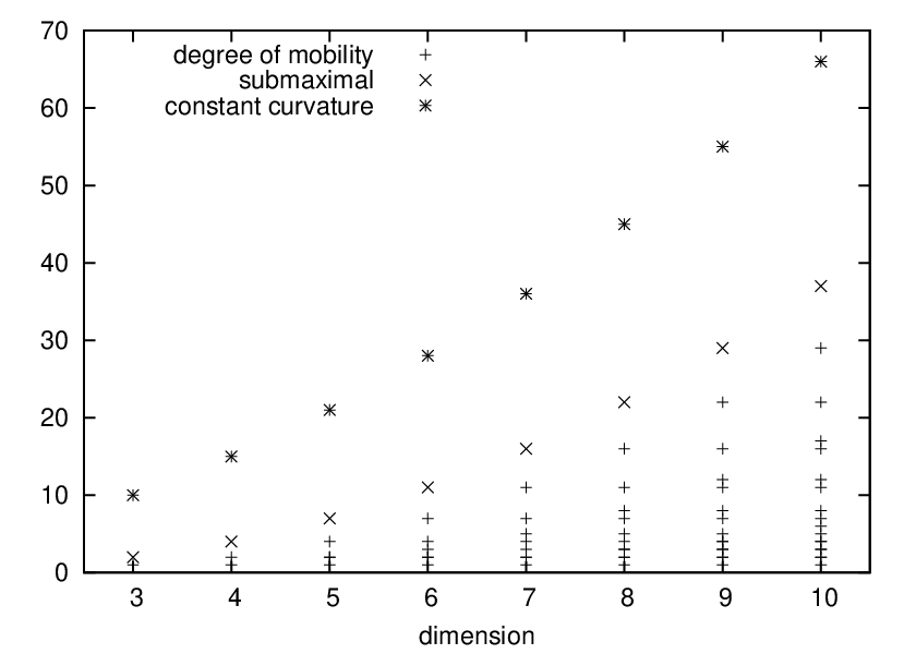
The Riemannian version of Theorem 1 is known and is due to [23, 9]: the principle idea is due to [23], but the main result has a mistake which was corrected in [9].

We see that the biggest degree of mobility of a metric of a nonconstant curvature on a simply-connected manifold is $\tfrac{(n-1)(n-2)}{2}+1=\tfrac{(n-3)n}{2}+2$ . This value is known to be the ‘‘submaximal’’ value for metrics of all signatures, see [20, §1.2] and [7, Theorem 6.2]. As we mentioned above, the maximal value of the degree of mobility of a metric on an $n$ -dimensional manifold is achieved on simply-connected manifolds of constant sectional curvature and is equal to $\tfrac{(n+2)(n+1)}{2}$ .

Let us now comment on our assumptions in Theorem 1. The assumption that the manifold is simply-connected is important: the degree of mobility of an isometric quotient can be smaller than the degree of mobility of the initial manifold. For example, for certain isometric quotients of the round 3-sphere, the degree of mobility could be one, [16]. The assumption $n\geq 3$ is also important: the dimension $n=2$ was studied already by Darboux [5] and Koenigs [10], see also [3, 13]. They have shown that in dimension $n=2$ the degree of mobility of an arbitrary metric of nonconstant curvature is 1,2,3,4. We see that the list of possible degrees of mobility in dimension 2 is very different from the list obtained by the formula $D(g)=\frac{k(k+1)}{2}+\ell$ from Theorem 1.

The assumption that there exists a metric that is geodesically equivalent to $g$ but not affinely equivalent to $g$ is also important since one can construct examples of metrics (of arbitrary signature) on $\mathbb{R}^{n}$ with the degree of mobility equal to $\tfrac{(n-4)(n-3)}{2}+2$ , and for $n\geq 5$ this number is not in the list of degrees of mobility given by Theorem 1. Of course, in the lorentzian signature, all metrics geodesically equivalent to the metrics from these examples are affinely equivalent to them.

Unfortunately, we do not know whether the assumption that the metric has riemannian or lorentzian signature is important. In dimension $n=3$ , all metrics have, up to multiplication by $-1$ , the riemannian or lorentzian signature. In dimension $n=4$ one can show that the statement of our theorem still holds (was essentially done in [7]). Our proof does not work for metrics of other signatures though: we construct examples showing that one of the main tools of the proof, Theorem 5, is wrong if the initial metric has other signatures.

1.2. Application to the dimension of the projective algebra.

A vector field whose (local) flow takes unparameterized geodesics to geodesics is called a projective vector field. Projective vector fields satisfy the equation (161) in Section 2.1. Since the equation (161) is linear, the space of its solutions is a linear vector space, we will denote it by $proj(g)$ . Since every killing vector field (i.e., a vector field whose flow acts by (local) isometries) is evidently a projective vector field, the set of the Killing vector fields which we denote by $iso(g)$ forms a vector subspace of $proj(g)$ .

Theorem 3.

Let $(M^{n},g)$ be a connected simply-connected $n\geq 3$ -dimensional manifold of nonconstant curvature of riemannian or lorentzian signature. Assume that $D(g)\geq 3$ and that there exists at least one metric which is geodesically equivalent to $g$ , but not affinely equivalent to $g$ . Then,

\dim proj(g)-\dim iso(g)=\frac{k(k+1)}{2}+\ell-1

for certain $k\in\{0,1,...,n-2\}$ and $1\leq\ell\leq\lfloor\tfrac{n-k+1}{3}\rfloor$ .

In the case of $D(g)=2$ , we prove that the codimension of the space of homothety vector fields (i.e., such that $\mathcal{L}_{v}g=\operatorname{const}g$ ) in the space of projective fields is at most 1, see Lemma 17 is Section 8.2.

Note that the number $\dim proj(g)-\dim iso(g)$ is a natural number in the projective geometry. Indeed, since Knebelman [11, 17] it is known that if $\bar{g}$ is geodesically equivalent to $g$ then $\dim iso(g)=\dim iso(\bar{g})$ . Since evidently $\dim proj(g)=\dim proj(\bar{g})$ , we have $\dim proj(g)-\dim iso(g)=\dim proj(\bar{g})-\dim iso(\bar{g})$ .

Note that there is almost no hope to obtain the possible dimensions of $iso(g)$ (for manifolds of all dimensions), since the possible values of $\dim iso(g)$ for homogeneous manifolds give too many combinatorical possibilities. For every fixed dimension, it can be in principle done though. Moreover, as examples show, the lists of possible dimensions of $iso(g)$ on a simply-connected $n$ -dimensional manifold depend on the signature of $g$ and, for certain $n$ , are different for Riemannian and Lorentzian metrics.

1.3. Overview of known global results.

If the manifold $(M,g)$ is closed or the metrics are complete, the natural analog of Theorem 1 was known before and is true for metrics of all signature: by [8, Theorem 1], if two complete metrics $g$ and $\bar{g}$ of nonconstant curvature on a $n\geq 3$ -dimensional manifold are geodesically equivalent but not affinely equivalent, then $D(g)=2$ . By [18, Corollary 5.2], if two metrics $g$ and $\bar{g}$ of nonconstant curvature on a closed $n\geq 3$ -dimensional manifold are geodesically equivalent but not affinely equivalent, then $D(g)=2$ . If we merely assume that the metric $g$ is complete, then, in the riemannian and in the lorentzian case, the list of the degrees of mobilities (on connected simply-connected manifolds) coincides with that of in Theorem 1.

1.4. Relation to parallel symmetric $(0,2)$ -tensor fields and difficulties of the lorentzian signature.

The cone manifold over $(M,g)$ is the manifold $\widehat{M}=\mathbb{R}_{>0}\times M$ endowed with the metric $\hat{g}$ defined by $\hat{g}=\,dr^{2}+r^{2}g$ (i.e., in the local coordinate system $(r,x^{1},...,x^{n})$ on $\widehat{M}$ , where $r$ is the standard coordinate on $\mathbb{R}_{>0}$ , and $(x^{1},...,x^{n})$ is a local coordinate system on $M$ , the scalar product in $\hat{g}$ of the vectors $u=u^{0}{\partial_{r}}+\sum_{i=1}^{n}u^{i}{\partial_{x^{i}}}$ and $v=v^{0}{\partial_{r}}+\sum_{i=1}^{n}v^{i}{\partial_{x^{i}}}$ is given by $\hat{g}(u,v)=u^{0}v^{0}+r^{2}\sum_{i,j=1}^{n}g_{ij}u^{i}v^{j}$ ).

The degree of mobility of metrics on $n$ -dimensional manifold appears to be closely related to the dimension of the space of parallel symmetric $(0,2)$ -tensor fields of $n+1$ -dimensional cone manifolds. We will explain what we mean by ‘‘closely related’’ in Section 2. For Riemannian metrics, this observation was essentially known to Solodovnikov [25] and was used by Shandra in [23], where, as we mentioned above, the Riemannian version of our main Theorem 1 was essentially proved. In [8], the result of Solodovnikov was extended for all signatures, which allows us to use it in our problem. The assumption that the metric $g$ has lorentzian signature $(1,n-1)$ implies that the (metric of the) cone manifold which is used in the proof of Theorem 1 has signature $(1,n)$ or $(n-1,2)$ .

In view of this relation between geodesically equivalent metrics and parallel symmetric $(0,2)$ -tensor fields, the following statement is closely related to Theorem 1:

Theorem 4.

Let $(\widehat{M}^{n+1},\hat{g})$ be a connected simply-connected nonflat cone manifold of signature $(0,n+1)$ , $(1,n)$ or $(n-1,2)$ . Then, the dimension of the space of parallel symmetric $(0,2)$ -tensor fields is $\frac{k(k+1)}{2}+\ell$ , where $k$ is the dimension of the space of parallel vector fields, and $1\leq\ell\leq\lfloor\tfrac{n-k+1}{3}\rfloor$ .

Though Theorem 4 provides one of the main steps in the proof of Theorem 1, it is not equivalent to Theorem 1. Actually, Theorem 4 follows from Theorem 1, modulo certain results of [8, 18] we recall in Section 2.7. If the signature of $g$ is riemannian, Theorem 1 follows from Theorem 4, though this implication needs additional work which will be essentially done in Section 5.3.

If $g$ has lorentzian signature, proof of Theorem 1 splits into two parts: the first ‘‘generic’’ part is based on Theorem 4 and the second part (‘‘special case’’) is Lemma 13.

Let us now explain two main steps in the proof of Theorem 4, which are Theorems 5, 6 below. Besides providing an important step in the proof of Theorem 1, Theorem 5 could be interesting on its own since investigation of parallel tensor fields on cone manifolds is a classical topic, see for example [1, 6, 21].

Fix a point $p\in\widehat{M}$ (where $(\widehat{M},\hat{g})$ is a simply-connected cone manifold). Consider the holonomy group $Hol_{p}(\hat{g})\subset SO(T_{p}\widehat{M},\hat{g}_{p})$ of the metric $\hat{g}$ . Consider the decomposition of $T_{p}\widehat{M}$ in the direct product of mutually orthogonal $\hat{g}$ -nondegenerate subspaces invariant w.r.t. the action of the holonomy group

(1)

T_{p}\widehat{M}=V_{0}\oplus V_{1}\oplus...\oplus V_{\ell}.

We assume that $V_{0}$ is flat in the sense that the holonomy group acts trivially on $V_{0}$ , and that the decomposition is maximal in the sense that for all $i=1,...,\ell$ it is not possible to decompose $V_{i}$ into the direct product of two nontrivial (i.e., of dimension $\geq 2$ ) $\hat{g}$ -nondegenerate subspaces invariant w.r.t. the action of the holonomy group. We allow $\dim(V_{0})=0$ but assume $\dim(V_{i})\geq 2$ for $i\neq 0$ .

It is well known that parallel symmetric $(0,2)$ -tensor fields on a simply-connected manifold are in the one-to-one correspondence with bilinear symmetric $(0,2)$ -forms on $T_{p}\widehat{M}$ invariant with respect to $Hol_{p}(\hat{g})$ .

We denote by $g_{i}$ , $i=0,\dots,\ell$ , the restriction of the metric $g$ to the subspace $V_{i}$ , considered as a $(0,2)$ -tensor on $T_{p}M$ : for the vectors $v=v_{0}+v_{1}+...+v_{\ell}$ and $u=u_{0}+u_{1}+...+u_{\ell}$ of $T_{p}\widehat{M}$ (where $v_{\alpha},u_{\alpha}\in V_{\alpha}$ ) we put

g_{i}(v_{0}+v_{1}+...+v_{\ell},u_{0}+u_{1}+...+u_{\ell})=g(v_{i},u_{i}).

$g_{i}$ is evidently invariant w.r.t. $Hol_{p}(\hat{g})$ .

Theorem 5.

Let $(\widehat{M},\hat{g})$ be a simply-connected cone manifold of dimension $n+1$ . Assume $\hat{g}$ has signature $(1,n)$ , $(n-1,2)$ , or the riemannian signature $(0,n+1)$ , and consider the (maximal) decomposition (1). We denote by $\{\tau_{1},...,\tau_{k}\}$ a basis in the space of 1-forms on $T_{p}\widehat{M}$ that are invariant with respect to the holonomy group.

Let $A$ be a symmetric bilinear form on $T_{p}\widehat{M}$ such that it is invariant with respect to the holonomy group. Then, there exists a symmetric $k\times k$ -matrix $c_{ij}\in\mathbb{R}^{k^{2}}$ and constants $C_{1},...,C_{\ell}\in\mathbb{R}$ such that

(2)

A=\sum_{i,j=1}^{k}c_{ij}\tau_{i}\tau_{j}+\sum_{i=1}^{\ell}C_{i}g_{i}.

Evidently, any bilinear form $A$ given by the formula (2) is invariant with respect to the holonomy group and is symmetric.

In the case when the metric $\hat{g}$ is Riemannian, Theorem 5 is well-known and is essentially due to de Rham [22]. Moreover, in this case it is true without the assumption that $(\widehat{M},\hat{g})$ is a cone manifold. The classical way to formulate Theorem 5 in the Riemannian setup is as follows: there exists a coordinate system

x=(\underbrace{x_{0}^{1},...,x_{0}^{k_{0}}}_{\bar{x}_{0}},\underbrace{x_{1}^{1},...,x_{1}^{k_{1}}}_{\bar{x}_{1}},...,\underbrace{x_{\ell}^{1},...,x_{\ell}^{k_{\ell}}}_{\bar{x}_{\ell}})

in a neighborhood of $p$ such that in this coordinate system the metric has the block-diagonal form (with the blocks of dimensions $k_{0}\times k_{0}$ , … , $k_{\ell}\times k_{\ell}$ )

\hat{g}=\begin{pmatrix}g_{0}&&\\ &g_{1}&&\\ &&\ddots&\\ &&&g_{\ell}\end{pmatrix}

such that the entries of each matrix $g_{i}$ depend on the coordinates $x_{i}^{1},...,x_{i}^{k_{i}}$ only, such that the metric $g_{0}$ is the flat metric $(dx_{0}^{1})^{2}+...+(dx^{k_{0}}_{0})^{2}$ , and such that the holonomy group of each metric $g_{i}$ for $i\neq 0$ is irreducible. For this metric, every symmetric bilinear form invariant with respect to the holonomy group is given by

(3)

A=\sum_{i,j=1}^{k_{0}}c_{ij}dx_{0}^{i}\,dx_{0}^{j}+\sum_{i=1}^{\ell}C_{i}g_{i},

where $c_{ij}$ is a symmetric $k_{0}\times k_{0}$ -matrix. The relation between the formulas (2) and (3) is as follows: in the formula (3), the 1-forms invariant with respect to $Hol_{p}(\hat{g})$ are (essentially) the one-forms on $V_{0}$ (and therefore $k=k_{0}=dim(V_{0})$ and as the basis in the space of 1-forms invariant w.r.t. $Hol_{p}(\hat{g})$ we can take $dx_{0}^{1},...,dx_{0}^{k_{0}}$ ). In the other signatures, there may exist invariant one-forms on $T_{p}\widehat{M}$ that are not 1-forms on $V_{0}$ .

In the case when the metric $\hat{g}$ has lorentzian signature, Theorem 5 is also known (see for example [12]) and is also true without the assumption that $(\widehat{M},\hat{g})$ is a cone manifold. The new part of Theorem 5 is when the signature is $(n-1,2)$ , as example 1 in Section 3.3.3 shows, in this case the assumption that the metric is a cone metric is essential.

Moreover, the assumption that the signature of the metric $g$ is riemannian, lorentzian, or $(n-1,2)$ is important for Theorem 5, see (counter)example 2 in Section 3.3.3.

Theorem 5 describes all parallel symmetric $(0,2)$ -tensor fields on cone manifolds of signatures $(0,n+1)$ , $(1,n)$ and $(n-1,2)$ . The next theorem counts the dimensions of the space of such tensor fields.

Theorem 6.

Under the assumptions of Theorem 5, the number $k$ is at most $n-2$ and the number $\ell$ is at least $1$ and at most $\lfloor\tfrac{n-k+1}{3}\rfloor$ .

Combining Theorems 5 and 6, we obtain Theorem 4. Now, as we explained above, Theorem 4 is essentially equivalent to the ‘‘generic’’ part of the Theorem 1; and the ideas used in the proof of Theorem 5, 6 will also be seen in the ‘‘special’’ part of the proof of Theorem 1.

2. Degree of mobility as the dimension of the space of parallel symmetric $(0,2)$ tensor fields on the cone.

2.1. Geodesically equivalent metrics, Sinjukov equation, and degree of mobility.

Whenever the tensor index notation are used, we consider $g$ as the background metric (to low and rise indexes), sum with respect to repeating indexes, and denote by comma ‘‘,’’ the covariant differentiation w.r.t. the Levi-Civita connection of $g$ . The dimension of our manifold will be denoted by $n$ ; we assume $n\geq 3$ .

As it was known already to Levi-Civita [15], two connections $\nabla=\Gamma_{jk}^{i}$ and $\bar{\nabla}=\bar{\Gamma}_{jk}^{i}$ have the same unparameterized geodesics, if and only if their difference is a pure trace: there exists a 1-form $\phi$ such that

(4)

\bar{\Gamma}_{jk}^{i}-\Gamma_{jk}^{i}=\delta_{k}^{i}\phi_{j}+\delta_{j}^{i}\phi_{k}.

If $\nabla$ and $\bar{\nabla}$ related by (4) are Levi-Civita connections of metrics $g$ and $\bar{g}$ , then one can find explicitly (following Levi-Civita [15]) a function $\phi$ on the manifold such that its differential $\phi_{,i}$ coincides with the 1-form $\phi_{i}$ : indeed, contracting (4) with respect to $i$ and $j$ , we obtain $\bar{\Gamma}_{pi}^{p}=\Gamma_{pi}^{p}+(n+1)\phi_{i}$ . On the other hand, for the Levi-Civita connection $\nabla$ of a metric $g$ we have $\Gamma_{pk}^{p}=\tfrac{1}{2}\frac{\partial\log(|det(g)|)}{\partial x_{k}}$ . Thus,

(5)

\phi_{i}=\frac{1}{2(n+1)}\tfrac{\partial}{\partial x_{i}}\log\left(\left|\tfrac{\det(\bar{g})}{\det(g)}\right|\right)=\phi_{,i}

for the function $\phi:M\to\mathbb{R}$ given by

(6)

\phi:=\tfrac{1}{2(n+1)}\log\left(\left|\tfrac{\det(\bar{g})}{\det(g)}\right|\right).

In particular, the derivative of $\phi_{i}$ is symmetric, i.e., $\phi_{i,j}=\phi_{j,i}$ .

The formula (4) implies that two metrics $g$ and $\bar{g}$ are geodesically equivalent if and only if for a certain $\phi_{i}$ (which is, as we explained above, the differential of $\phi$ given by (6)) we have

(7)

\bar{g}_{ij,k}-2\bar{g}_{ij}\phi_{k}-\bar{g}_{ik}\phi_{j}-\bar{g}_{jk}\phi_{i}=0,

where ‘‘comma’’ denotes the covariant derivative with respect to the connection $\nabla$ . Indeed, the left-hand side of this equation is the covariant derivative with respect to $\bar{\nabla}$ , and vanishes if and only if $\bar{\nabla}$ is the Levi-Civita connection for $\bar{g}$ .

The equations (7) can be linearized by a clever substitution: consider $a_{ij}$ and $\lambda_{i}$ given by

(8)		$\displaystyle a_{ij}$	$\displaystyle=$	$\displaystyle e^{2\phi}\bar{g}^{pq}g_{pi}g_{qj},$
(9)		$\displaystyle\lambda_{i}$	$\displaystyle=$	$\displaystyle-e^{2\phi}\phi_{p}\bar{g}^{pq}g_{qi},$

where $\bar{g}^{pq}$ is the tensor dual to $\bar{g}_{pq}$ : $\bar{g}^{pi}\bar{g}_{pj}=\delta_{j}^{i}$ . It is an easy exercise to show that the following linear equations for the symmetric $(0,2)$ -tensor $a_{ij}$ and $(0,1)$ -tensor $\lambda_{i}$ are equivalent to (7):

(10)

a_{ij,k}=\lambda_{i}g_{jk}+\lambda_{j}g_{ik}.

One may consider the equation (10) as a linear PDE-system on the unknown $(a_{ij},\lambda_{k})$ ; the coefficients in this system depend on the metric $g$ .

One can also consider (10) as a linear PDE-system on the components of the tensor $a_{ij}$ only, since the components of $\lambda_{i}$ can be obtained from the components of $\nabla_{k}a_{ij}=a_{ij,k}$ by linear algebraic manipulations. Indeed, multiplying (10) by $g^{ij}$ we obtain

(11)

\displaystyle\lambda_{k}=\tfrac{1}{2}(a_{ij}g^{ij})_{,k}=\tfrac{1}{2}\left(\operatorname{Tr}_{g}(a)\right)_{,k}

Since (10) is a system of linear PDE, the set of its solutions is a linear vector space. Its dimension will be called the degree of mobility of $g$ and denoted by $D(g)$ . Clearly, $D(g)\geq 1$ , since $a_{ij}=g_{ij}$ is a solution of (10). It is known (see for example [24, p.134]) that $D(g)\leq\tfrac{(n+1)(n+2)}{2}$ .

2.2. Metrics with $D(g)\geq 3$ , extended system, and plan of the proof of Theorem 1.

Theorem 7 ([8]).

Let $(M^{n},g)$ , $n\geq 3$ , be a connected pseudo-Riemannian manifold such that $D(g)\geq 3$ . Then there exists a constant $B$ such that for every solution $(a_{ij},\lambda_{i})$ of (10) there exists a smooth function $\mu$ such that the following system

\displaystyle\left\{\begin{array}[]{ll}a_{ij,k}&=\lambda_{i}g_{jk}+\lambda_{j}g_{ik}\\ \lambda_{i,j}&=\mu g_{ij}+Ba_{ij}\\ \mu_{,i}&=2B\lambda_{i}\end{array}\right.

is satisfied.

Thus, the degree of mobility of the metric $g$ is equal to the dimension of the space of solutions $(a,\lambda,\mu)$ of the ‘‘extended system’’ (7).

Note that the constant $B$ is a metric invariant of $g$ (in the sense that a metric can not have two nontrivial solutions with different $B$ , see [8, §2.3.5]) but it is not a projective invariant: for a metric $\bar{g}$ that is geodesically equivalent to $g$ we may have $\bar{B}:=B(\bar{g})\neq B$ (see Section 5.3).

In Section 2.7 we reduce the case $B\neq 0$ to $B=-1$ and then show that the solutions of (7) and parallel symmetric $(0,2)$ -tensor fields on the cone manifold are in one-to-one correspondence. In this setting, Theorem 1 follows from Theorems 5, 6.

In the case $B=0$ we consider two subcases. In Section 5, we assume that the extended system (7) admits a solution $(a,\lambda,\mu)$ with $\mu\not\equiv 0$ . In this subcase we can (locally) find a metric $\bar{g}$ that is geodesically equivalent to $g$ , has the same signature as $g$ and such that $\bar{B}=B(\bar{g})<0$ . Since evidently $D(\bar{g})=D(g)$ and the case $B\neq 0$ has been already solved, we are done (though some additional work is required to make a transition ‘‘local’’ $\rightarrow$ ‘‘on a simply connected manifold’’, see Section 5.4 for details).

Finally, in Section 6 we consider the ‘‘special’’ case, when the extended system admits only solutions $(a,\lambda,\mu)$ with $\mu=0$ . In this case all metrics $\bar{g}$ geodesically equivalent to $g$ have $\bar{B}=0$ . In Section 6, we study and describe such metrics, calculate their degrees of mobility, and show that they are still in the list from Theorem 1.

2.3. Metric cone and its Levi-Civita connection.

By the metric cone over $(M,g)$ we understand the product manifold $\widehat{M}=\mathbb{R}_{{}>0}(r)\times M(x)$ equipped by the metric $\hat{g}$ such that in the coordinates $(r,x)$ its matrix has the form

\displaystyle\hat{g}(r,x)=\left(\begin{array}[]{cc}1&0\\ 0&r^{2}g(x)\end{array}\right).

The coordinates such that a metric has the form (2.3) will be called the cone coordinates.

For further use we calculate the Levi-Civita connection on $\widehat{M}$ in the cone coordinates.

Lemma 1 (Folklore, see for example [1, 18]).

Levi-Civita connection $\widehat{\nabla}=\{\widehat{\Gamma}^{{\tilde{\imath}}}_{{\tilde{\jmath}}{\tilde{k}}}\}$ corresponding to metric $\hat{g}$ on $\widehat{M}$ is given by formula:

(17)		$\displaystyle\widehat{\Gamma}^{0}_{00}=0,\ \widehat{\Gamma}^{i}_{00}=0,$
(18)		$\displaystyle\widehat{\Gamma}^{0}_{j0}=\widehat{\Gamma}^{0}_{0k}=0,$
(19)		$\displaystyle\widehat{\Gamma}^{i}_{j0}=\frac{1}{r}\,\delta^{i}_{j},\qquad\widehat{\Gamma}^{i}_{0k}=\frac{1}{r}\,\delta^{i}_{k},$
(20)		$\displaystyle\widehat{\Gamma}^{0}_{jk}={}-r\cdot g_{jk}(x),$
(21)		$\displaystyle\widehat{\Gamma}^{i}_{jk}=\Gamma^{i}_{jk}(x),$

where $\Gamma^{i}_{jk}$ are Christoffel symbols of the Levi-Chivita connection determined by metric $g$ on $M$ , and indicies $i,j,k$ take values from $1$ to $n$ .

Proof.

It is an easy exercise: we substitute the components of $\hat{g}$ in the formula:

\widehat{\Gamma}^{{\tilde{\imath}}}_{{\tilde{\jmath}}{\tilde{k}}}=\frac{1}{2}\,\hat{g}^{{\tilde{\imath}}{\tilde{\alpha}}}\left({}-\frac{\partial\hat{g}_{{\tilde{\jmath}}{\tilde{k}}}}{\partial x^{{\tilde{\alpha}}}}+\frac{\partial\hat{g}_{{\tilde{\alpha}}{\tilde{k}}}}{\partial x^{{\tilde{\jmath}}}}+\frac{\partial\hat{g}_{{\tilde{\jmath}}{\tilde{\alpha}}}}{\partial x^{{\tilde{k}}}}\right)

and put ${\tilde{\imath}},{\tilde{\jmath}},{\tilde{k}}$ to be equal to 0 or to certain $i,j,k$ respectively. ∎

2.4. Cone structure as the existence of a positive solution of (2).

Lemma 2.

Pseudo-Riemannian $n+1$ -dimensional manifold $(\widehat{M},\hat{g})$ is locally isometric to a cone manifold if and only if, for any $P\in\widehat{M}$ there exists a positive function $v$ on $U(P)$ such that

\displaystyle\left\{\begin{array}[]{c}v_{,ij}=\hat{g}_{ij},\\ v_{,i}\,v_{,}\vphantom{v}^{i}=2v.\end{array}\right.

Proof.

$\Rightarrow$ Let $(\widehat{M},\hat{g})$ be locally the cone over $(M,g)$ . Then there exist coordinates $(r,x)$ , such that $\hat{g}$ has the form (2.3). By direct calculations we see that the function $v=\frac{1}{2}r^{2}$ satisfies (2).

$\Leftarrow$ Suppose $v$ is a positive function in $U(P)$ satisfying (2). We consider $r=\sqrt{2v}$ and its gradient $r_{,}^{\ i}$ . By direct calculation, we see

r_{,i}\,r_{,}\vphantom{r}^{i}=\frac{v_{,i}}{\sqrt{2v}}\cdot\frac{v_{,}\vphantom{v}^{i}}{\sqrt{2v}}=\frac{1}{2v}\cdot 2v=1.

This in particular implies that the differential of $r$ nowhere vanishes.

Consider the $n$ -dimensional hypersurface $S$ defined by the equation $r=r(P)$ . Let $(x_{1},\dots,x_{n})$ be a local coordinate system on $S$ .

Let us now use $r$ and the coordinates $(x_{1},...,x_{n})$ to construct a coordinate system in a neighborhood $P$ . More precisely, for every point $Q=(x_{1},\dots,x_{n})\in S$ there exists the unique curve $\gamma_{Q}:(r(P)-\varepsilon,r(P)+\varepsilon)\to\widehat{M}$ such that

\dot{\gamma_{Q}}^{i}(t)=r_{,}^{\ i}\mbox{ and }\gamma_{Q}(r(P))=Q.

Clearly, the mapping $(t,Q)\mapsto\gamma_{Q}(t)$ is a local diffeomorphism and therefore defines a coordinate system $(t,x_{1},...,x_{n})$ in a neighborhood of $P$ . Because $r_{,}^{\ i}$ is the gradient of $r$ , the value of the function $r$ at the points $\gamma_{Q}(t)$ is equal to $r$ , so this coordinate system actually reads $(r,x_{1},\dots,x_{n})$ .

Let us now show that in these coordinates the metric $\hat{g}$ has the form (2.3). Using (2), we calculate

r_{,ij}=\widehat{\nabla}_{j}\left(\frac{v_{,i}}{r}\right)=\frac{1}{r}(\hat{g}_{ij}-r_{,i}r_{,j}).

By the construction of the coordinates $(r,x)$ , we have

(24)

\partial_{r}\hat{g}_{ij}={\mathcal{L}}_{\partial_{r}}(g_{ij})=2r_{,ij}=\frac{2}{r}(\hat{g}_{ij}-r_{,i}r_{,j})

For $i,j\neq 0$ the equation (24) reads $\partial_{r}\hat{g}_{ij}=\frac{2}{r}\hat{g}_{ij}$ . This equation could be viewed as an ODE; solving it we obtain $\hat{g}_{ij}(r,x)=r^{2}g_{ij}(x)$ , where $g_{ij}(x)$ is the restriction of the metric $\hat{g}$ to $S$ written in the coordinates $x_{1},...,x_{n}$ . Since the $r_{,}^{\ i}$ is the gradient of $r$ and therefore is orthogonal to $\{(r,x_{1},...,x_{n})\mid r=\operatorname{const}\}$ , we have $\hat{g}_{0j}=\hat{g}_{i0}=0.$ Now, $\hat{g}_{00}=r_{,i}r_{,}\vphantom{r}^{i}=1$ . Combining all these, we see that in the coordinates $(r,x_{1},\dots,x_{n})$ the metric $\hat{g}$ is given by (2.3). ∎

Remark 1.

From the first equaiton of (2) we see that a solution $v$ of (2) has nonzero differential at every point of a certain everywhere dense open subset of $M$ . Then, $v$ is not zero at every point of a certain everywhere dense open subset of $M$ . By Lemma 2, near the points where $v$ is positive, $g$ is isometric to a cone metric. Since, for a negative solution $v$ for $g$ the (positive) function $-v$ is a solution of (2) for $g^{\prime}=-g$ , the metric $-g$ is locally a cone metric.

Remark 2.

Actually, the first equation of (2) almost implies the second. Indeed, if $v$ satisfies the first equation of (2), then the function $\tfrac{1}{2}v_{,}^{\ i}v_{,i}$ has differential $\left(\tfrac{1}{2}v_{,}^{\ i}v_{,i}\right)_{,k}=v_{,}^{\ i}g_{ik}=v_{,k}$ implying that for a certain constant $C$ the function $v+C$ satisfies (2). Moreover, if a 1-form $v_{i}$ satisfies $v_{i,j}=g_{ij}$ , then it is closed so there exists a function $v$ such that $v_{,i}=v_{i}$ provided the manifold is simply connected.

2.5. Properties of the cone vector field.

By Lemma 2, cone manifolds are (locally) characterized by the existence of a positive function $v$ satisfying (2). Its gradient $\vec{v}:=v_{,}^{\ i}$ will be called a cone vector field.

Lemma 3.

Let $(M,g)$ be a $2$ -dimensional manifold, and let $v_{i}$ be a $1$ -form such that $v_{i,j}=g_{ij}$ . Then, $M$ is flat.

Proof.

By the second equation of (2), $v_{i}\neq 0$ on an everywhere dense open subset of $M$ . Take a point $P\in\widehat{M}$ from this subset and choose a basis in $T_{p}\widehat{M}$ such that in this basis $\vec{v}:=v_{,}^{\ i}=\left(\begin{array}[]{cc}1\\ 0\end{array}\right)$ . By the definition of the Riemannian curvature $R^{i}_{\ jk\ell}$ , we have

(25)

\displaystyle R^{i}_{\ 1k\ell}=R^{i}_{\ jk\ell}v^{j}{=}\nabla_{k}\nabla_{\ell}v^{j}-\nabla_{k}\nabla_{l}v^{j}\stackrel{{\scriptstyle\eqref{eq:hom}}}{{=}}\nabla_{k}\delta^{j}_{\ell}-\nabla_{\ell}\delta^{j}_{k}=0\quad\mbox{for all $i,k,l=1,2.$}

Then, by the symmetries of the Riemannian curvature tensor we see that the component $R_{ijk\ell}=0$ , when $i,j,k$ or $\ell$ is equal to $1$ . Since the only remaining component $R_{2222}$ is also zero, $R^{i}_{\ jk\ell}\equiv 0$ and the metric $g$ is flat. ∎

Lemma 4.

Assume $v$ satisfies (2). Then, for any parallel vector field $u\neq 0$ , for every point $P\in M$ such that the Riemannian curvature tensor $R^{i}_{\ jk\ell}$ is not zero, the vectors $\vec{v}:=v_{,}^{\ i}$ and $u^{i}$ are not proportional at $P$ .

Proof.

As we explained in the proof of Lemma 3, see (25) there, we have $v_{,i}R^{i}_{\ jk\ell}=0$ . We covarinatly differentiate this equation to obtain:

v_{i,m}R^{i}_{\ jk\ell}+v_{,i}R^{i}_{\ jk\ell,m}=0\ \ \textrm{implying}\ \ R_{mjk\ell}+v_{,i}R^{i}_{\ jk\ell,m}=0.

Since $R_{mjk\ell}\neq 0$ at $P$ , we have

(26)

v_{,i}R^{i}_{\ jk\ell,m}\neq 0.

But by definition of $R^{i}_{\ jk\ell}$ , for any parallel vector field $u$ we have $u^{j}R^{i}_{\ jk\ell}=\nabla_{k}\nabla_{\ell}u^{j}-\nabla_{k}\nabla_{\ell}u^{j}=0$ . Covariantly differentiating the last equation and using the symmetries of the curvature tensor, we obtain $u_{i}R^{i}_{\ jk\ell,m}=0$ . Combining this with (26), we see that the vectors $u$ and $\vec{v}$ are not proportional. ∎

2.6. Direct product and decomposition of cone manifolds.

Lemma 5.

Consider the direct product

(\widehat{M},\hat{g})=(M_{1},\overset{1}{g})\times(M_{2},\overset{2}{g})

and assume that a function $v$ on $\widehat{M}$ satisfies (2).

Then, for any $s=1,2$ there exists a function $\overset{s}{v}$ von $M_{s}$ satisfying (2) (w.r.t. the metric $\overset{s}{g}$ on $M_{s}$ ). The differential $\overset{s}{v}_{,i}=d\overset{s}{v}$ of the function $\overset{s}{v}$ is not zero at almost every point. Moreover, $\overset{s}{v}_{,i}R^{i}_{\ jkm}=0$ , where $R$ is the curvature tensor of $\hat{g}$ .

Remark 3.

Withing the whole paper we understand ‘‘almost everywhere’’ or ‘‘at almost every point’’ in the topological sense: a property is fulfilled almost everywhere or at almost every point if the set of the points where it is fulfilled is open and everywhere dense.

Proof.

Let us consider the decomposition $v_{,i}=\overset{1}{v}_{i}+\overset{2}{v}_{i}\,,$ where $\overset{s}{v}_{i}$ is the orthogonal projection of $v_{i}$ to $TM_{s}$ . Let us choose coordinates $x_{1},...,x_{n}$ on $M$ such that $x_{1},\dots,x_{k}$ are coordinates on $M_{1}$ and $x_{k+1},\dots,x_{n}$ are coordinates on $M_{2}$ . For $i,j\leq k$ we have

\overset{1}{\nabla}_{j}\overset{1}{v}_{i}=\widehat{\nabla}_{j}v_{i}=g_{ij}=\overset{1}{g}_{ij}

implying that the components of $\overset{1}{v}_{i}$ depends on the coordinates $x_{1},\dots,x_{k}$ only and could be viewed as a 1-form on $M_{1}$ . Next, consider the function $\overset{1}{v}:=\tfrac{1}{2}\overset{1}{v}_{i}{\overset{1}{v}}{}^{i}$ which also depend on the coordinates $x_{1},\dots,x_{k}$ only and can be viewed as a function on $M_{1}$ . We have

\overset{1}{v}_{,i}=\tfrac{1}{2}\left(\overset{1}{v}_{k}{\overset{1}{v}}{}^{k}\right)_{,i}=\overset{1}{g}_{ik}\overset{1}{v}{}^{k}=\overset{1}{v}_{i}.

Thus, $\overset{1}{v}$ satisfies (2). Similarly we can prove the existence of a function $\overset{2}{v}$ on $M_{2}$ satisfying (2).

The first equation of (2) implies that the differentials of $\overset{s}{v}_{i}$ are nonzero at almost every point.

Since the curvature tensor of $\hat{g}$ is the direct sum of the curvature tensors of $\overset{1}{g}$ and $\overset{2}{g}$ , and since as we explained in the proof of Lemma 3, $\overset{s}{v}_{,i}$ satisfies $\overset{s}{v}_{,i}\overset{s}{R}{}^{i}_{\ jkm}=0$ , where $\overset{s}{R}{}^{i}_{\ jkm}$ is the curvature tensor of $\overset{s}{g}$ , we have $\overset{s}{v}_{,i}R^{i}_{\ jkm}=0$ . ∎

Remark 4.

In Lemma 5 we do not require that the functions (which were denoted by $\overset{1}{v}$ , $\overset{2}{v}$ in the proof) on the manifolds $M_{1},M_{2}$ are positive. It is easy to construct an example such that $\overset{1}{v}$ is positive and $\overset{2}{v}$ is negative.

Lemma 6.

Assume $(\widehat{M},\hat{g})$ is the direct product of two manifolds,

(\widehat{M},\hat{g})=(M_{1},\overset{1}{g})\times(M_{2},\overset{2}{g}),

where every $(M_{i},\overset{i}{g})$ , $i=1,2$ , is a cone manifold. Then, $(\widehat{M},\hat{g})$ admits a positive function satisfying (2).

Proof.

By Lemma 2, there exists positive functions $u(x)$ on $M_{1}$ and $v(y)$ on $M_{2}$ such that

\displaystyle\begin{array}[]{cc}u_{,ij}=\overset{1}{g}_{ij},&v_{,ij}=\overset{2}{g}_{ij},\\ u_{,i}u^{,i}=2u,&v_{,i}v_{,}^{\ i}=2v.\end{array}

Then, the function $w(x,y)=u(x)+v(y)$ is a positive function on $\widehat{M}$ and satisfies (2). Indeed,

w_{,ij}=\left(\begin{array}[]{cc}u_{,ij}&0\\ 0&v_{,ij}\end{array}\right)=\hat{g}_{ij}

and $w_{,i}w^{,i}=u_{,i}u_{,}^{\ i}+v_{,i}v_{,}^{\ i}=2u+2v=2w$ . ∎

Remark 5.

Both Lemmas above are true for the direct products of arbitrary number of manifolds: the proofs survive without any changes.

2.7. Solutions of the extended system with $B\neq 0$ as parallel $(0,2)$ -tensor fields on the cone.

Let $(M,g)$ be a connected $n\geq 3$ -dimensional pseudo-Riemannian manifold with $D(g)\geq 3$ . We consider the extended system (7) and assume $B\neq 0$ .

By Theorem 7, the degree of mobility of $g$ is equal to the dimension of the space of solutions of (7). Our goal is to construct an isomorphism between the space of the solutions of (7) and the space of parallel symmetric $(0,2)$ -tensor fields on a cone manifold.

First we renormalize the metric in order to obtain $B=-1$ .

Lemma 7.

Let $(a_{ij},\lambda_{i},\mu)$ satisfy (7) with $B\neq 0$ . Then, $(a^{\prime}_{ij}:=-Ba,,\lambda^{\prime}_{i}:=\lambda_{i},\mu^{\prime}:=-\tfrac{1}{B}\mu)$ satisfies (7) for the metric $g^{\prime}=-\tfrac{1}{B}g$ and $B(g^{\prime})=B^{\prime}=-1$ .

Proof.

We substitute $(a^{\prime}_{ij}:=-Ba,,\lambda^{\prime}_{i}:=\lambda_{i},\mu^{\prime}:=-\tfrac{1}{B}\mu)$ and $g^{\prime}=-\tfrac{1}{B}g$ in the system

\displaystyle\left\{\begin{array}[]{ll}a^{\prime}_{ij,k}&=\lambda^{\prime}_{i}g^{\prime}_{jk}+\lambda^{\prime}_{j}g^{\prime}_{ik}\\ \lambda^{\prime}_{i,j}&=\mu^{\prime}g^{\prime}_{ij}-a^{\prime}_{ij}\\ \mu^{\prime}_{,i}&=-2\lambda^{\prime}_{i}\end{array}\right.

and see that it is fulfilled. ∎

Thus, if $B\neq 0$ , we can assume $B=-1$ . In this setting the system (7) reads

\displaystyle\left\{\begin{array}[]{ll}a_{ij,k}&=\lambda_{i}g_{jk}+\lambda_{j}g_{ik}\\ \lambda_{i,j}&=\mu g_{ij}-a_{ij}\\ \mu_{,i}&=-2\lambda_{i}\end{array}\right.

Theorem 8 ([18]).

If a symmetric tensor field $a_{ij}$ on $(M,g)$ satisfies (2.7), then the $(0,2)$ -tensor field $A$ on $(\widehat{M},\hat{g})$ defined in the local coordinates $(r,x)$ by the following (symmetric) matrix:

\displaystyle A=\left(\begin{array}[]{c|ccc}\mu(x)&-r\lambda_{1}(x)&\dots&-r\lambda_{n}(x)\\ \hline\cr-r\lambda_{1}(x)&&&\\ \vdots&&r^{2}a(x)&\\ -r\lambda_{n}(x)&&&\end{array}\right),

is parallel with respect to the Levi-Civita connection of $\hat{g}$ .

Moreover, if a symmetric $(0,2)$ -tensor $A_{ij}$ on $\widehat{M}$ is parallel, then in the cone coordinates it has the form (8), where $(a_{ij},\lambda_{i},\mu)$ satisfy (2.7).

Proof.

This is an easy exercise (a straightforward way to do this exercise is to write down the condition that a symmetric parallel $(0,2)$ -tensor field on the cone is parallel, and compare it with (2.7)). ∎

3. Proof of Theorem 5.

3.1. Plan of the proof.

We consider the cone $(\widehat{M},\hat{g})$ of dimension $n+1\geq 4$ over connected simply connected $(M,g)$ . For every $(0,2)$ -tensor field $A_{ij}$ on $\widehat{M}$ we consider the $(1,1)$ -tensor field $L=L^{i}_{j}$ given by

(39)

A(.,.)=\hat{g}(L.,.),\textrm{ i.e., in coordinates\ }L^{i}_{j}=\hat{g}^{ik}A_{kj}.

We will view $L$ as a field of endomorphisms of $T\widehat{M}$ . If $A$ is parallel and symmetric, $L$ is parallel and selfadjoint, and vise versa.

Take $p\in\widehat{M}$ and consider the maximal orhtogonal decomposition of the tangent space $T_{p}\widehat{M}$ into the direct sum of nondegenerate subspaces invariant w.r.t. the action of the holonomy group:

(40)

T_{p}\widehat{M}=V_{0}\oplus V_{1}\oplus\dots\oplus V_{\ell}.

We assume that $V_{0}$ is flat, in the sense that the holonomy group acts trivially on $V_{0}$ , and that the decomposition is maximal, i.e., that each subspace $V_{a},a\geq 1$ , has no invariant $\hat{g}$ -nondegenerate subspaces, and, therefore, cannot be decomposed further.

We denote by $\overset{(\alpha)}{P}=\overset{(\alpha)}{P}{}^{j}_{i}$ the orthogonal projector onto $V_{\alpha},\alpha=0,\dots,\ell$ . $\overset{(\alpha)}{P}$ is selfadjoint and is preserved by the action of the holonomy group. It corresponds to $g_{a}$ from Theorem 5 via (39). Clearly, $(\overset{(0)}{P}+\dots+\overset{(\ell)}{P})=\operatorname{Id}$ . We consider the following decomposition of $L$ :

(41)

\displaystyle L=(\overset{(0)}{P}+\dots+\overset{(\ell)}{P})\,L\,(\overset{(0)}{P}+\dots+\overset{(\ell)}{P})=\sum_{a,b=0}^{\ell}\overset{(a)}{P}L\overset{(b)}{P}.

Each component $\overset{(a)}{P}L\overset{(b)}{P}$ is an endomorphism invariant w.r.t. the holonomy group. Moreover, if $a=b$ , then it is self-adjoint.

The proof of the Theorem 5 contains two parts: first, in Lemma 8 we show that each ‘‘non-diagonal’’ component $\overset{(a)}{P}L\overset{(b)}{P}$ , $a\neq b$ , is given by the quadratic combination of vectors and 1-forms invariant with respect to the holonomy group. This part will be purely algebraic. Then, in Section 3.3 we describe ‘‘diagonal blocks’’ $\overset{(a)}{P}L\overset{(a)}{P}$ and show that they are combinations of $\overset{(a)}{P}$ and quadratic combination of vectors and 1-forms invariant with respect to the holonomy group. These two parts imply Theorem 5, we explain it in Section 3.4.

3.2. Proof for ‘‘non-diagonal’’ components.

Lemma 8.

In the notation above, let $L^{\prime}=\overset{(a)}{P}L\overset{(b)}{P}$ , $a\neq b$ , be a ‘‘non-diagonal’’ component of $L$ (invariant w.r.t. to the holonomy group). Then, $L^{\prime}=\sum_{i,j}c_{ij}\tau_{i}^{*}\otimes\tau_{j},$ where $\tau_{s}\in T_{p}\widehat{M}$ are certain vectors invariant w.r.t. to the holonomy group, $\tau^{*}_{s}\in T^{*}_{p}\widehat{M}$ are certain $1$ -forms invariant w.r.t. to the holonomy group, and $c_{ij}\in\mathbb{R}$ are constants.

Proof.

Let $\bar{u}_{i},\dots,\bar{u}_{k}$ be a basis of $\operatorname{Im}L^{\prime}\subset V_{a}$ and $\bar{v}_{1},\dots\bar{v}_{r}$ be a basis in $V_{b}$ such that $L^{\prime}\bar{v}_{s}=\bar{u}_{s}$ for $s=1,...,k$ and and $\bar{v}_{k+1},\dots\bar{v}_{r}\in\ker L^{\prime}$ . Then,

(42)

L^{\prime}=\sum_{i\leq k}\bar{u}_{i}\otimes\bar{v}^{*}_{i},

where $v^{*}_{i}$ are the 1-forms dual to $v_{i}$ . It is known that the holonomy group $H_{p}$ is the direct product of the subgroups $H_{0}\times\dots\times H_{\ell}$ such that each $H_{\alpha}$ acts trivially on all $V_{\beta}$ such that $\beta\neq\alpha$ . Since $L^{\prime}(\widehat{M})\subset V(a)$ , for each $h=h_{0}\cdot...\cdot h_{l}\in H$ , $h_{\alpha}\in H_{\alpha}$ , and for any $v\in T_{p}\widehat{M}$ we have

h\,\underbrace{L^{\prime}(v)}^{\in V_{a}}=h_{a}\overset{(a)}{P}L\overset{(b)}{P}(v)=\overset{(a)}{P}Lh_{a}(\underbrace{\overset{(b)}{P}(v)}^{\in V_{b}})=\overset{(a)}{P}L\overset{(b)}{P}(v)=L^{\prime}(v)

Thus, all $\bar{u}_{i}\in\operatorname{Im}L^{\prime}$ are invariant with respect to the action of $H$ .

Similarly, consider the dual endomorphism $L^{\prime*}=\overset{(b)}{P^{*}}L^{*}\overset{(a)}{P^{*}}:V_{a}^{*}\to V_{b}^{*}$ and the action of the holonomy group $H$ on the dual decomposition:

h\,\underbrace{L^{\prime*}(u^{*})}^{\in V_{b}^{*}}=h_{b}\overset{(b)}{P^{*}}L^{*}\overset{(a)}{P^{*}}(u^{*})=\overset{(b)}{P^{*}}L^{*}h_{b}(\underbrace{\overset{(a)}{P^{*}}(u^{*})}^{\in V^{*}_{a}})=\overset{(b)}{P^{*}}L^{*}\overset{(a)}{P^{*}}(u^{*})=L^{\prime*}(u^{*})

Thus, $v_{s}^{*}=L^{\prime*}(u^{*}_{s}),s\leq k$ is invariant with respect to action of the holonomy group. Thus, all $v_{i}$ and $v^{*}_{i}$ from (42) are invariant w.r.t. holonomy group. ∎

3.3. Parallel symmetric tensor fields on indecomposable pseudo-Riemannian manifolds.

In this section we deal with the ‘‘diagonal’’ components $\overset{(a)}{P}L\overset{(a)}{P}$ of an arbitrary parallel self-adjoint tensor $L$ . We take $a\geq 1$ and denote by $M_{a}$ the $k_{a}$ -dimensional integral submanifold corresponding to the subspace $V_{a}$ and by $g_{a}$ the restriction of the metric to it. Clearly,

(1)

$M_{a}$ is indecomposable;
(2)

by Lemma 5, it admits a function satisfying (2)
(3)

if the signature of the initial metric $g$ is riemannian or lorentzian, then, by Lemma 7, the cone metric $\hat{g}$ has signature $(1,n)$ , $(n-1,2)$ , or the riemannian signature $(0,n+1)$ . Thus, the restriction $g_{a}$ of the cone metric to each component $M_{a}$ is either Riemannian, Lorentzian or has signature $(k_{a}-2,2)$ ;
(4)

The restriction of $\overset{(a)}{P}L\overset{(a)}{P}$ to $M_{a}$ is a well-defined parallel selfadjoint $(1,1)$ -tensor field on $M_{a}$ .

For readability we ‘‘forget’’ the index $a$ and denote the manifold $M_{a}$ , the metric $g_{a}$ on it and the restriction of $\overset{(a)}{P}L\overset{(a)}{P}$ to it by $\widehat{M}$ , $g$ and $L$ and assume that $k_{a}=\dim M_{a}=n+1$ ; they enjoy the properties (1–4) above.

The goal of the next two sections will be to prove that $L$ and the curvature tensor $R$ fulfill

(43)

L^{i}_{p}R^{p}_{\ jk\ell}=0.

In order to prove this result we will use the following property of parallel $(1,1)$ -tensor fields:

(44)

L^{i}_{p}R^{p}_{\ jk\ell}=R^{i}_{\ pk\ell}L^{p}_{j}.

In order to prove (44), we use that for the vector fields $X=\partial_{k},Y=\partial_{\ell},Z=\partial_{j}$ , in view of $[X,Y]=0$ , we have

R(X,Y)(Z)=\nabla_{X}\nabla_{Y}Z-\nabla_{Y}\nabla_{X}Z

Applying the (1,1)-tensor $L$ viewed as an endomorphism an using that it is parallel we obtain

L(R(X,Y)(Z))=L(\nabla_{X}\nabla_{Y}Z-\nabla_{Y}\nabla_{X}Z)=\nabla_{X}\nabla_{Y}L(Z)-\nabla_{Y}\nabla_{X}L(Z)=R(X,Y)(L(Z))

which is equivalent to (44).

Besides, we will use that for a solution $v$ of (2) and for the corresponding vector field $\vec{v}:=v_{,}^{\ i}$ we have $L^{k}\vec{v}\neq 0$ almost everywhere provided $L^{k}:=\underbrace{L\circ...\circ L}_{\textrm{$k$ times}}$ is not identically zero. Indeed, the existence of a solution of (2) implies that $g$ or $-g$ is a cone metric (in a neighbohood of almost every point). Then, by (8), $L^{i}_{j}\vec{v}^{j}=\pm\lambda^{i}$ . Now, by Theorem 7, the solutions $(a,\lambda,\mu)$ satisfy (7) and by assumptions we have $B=\pm 1$ . Therefore, if $\lambda^{i}$ is zero at every point of an open subset, $L$ is proportional to $\delta^{i}_{j}$ in this subset implying it is $\delta^{i}_{j}$ everywhere.

3.3.1. Possible Jordan forms of $L$ .

We first recall the following theorem from linear algebra:

Theorem 9 ([14], Theorem 12.2).

Let $g$ be a symmetric bilinear nondegenerate form on a $n$ -dimensional real linear vector space $V$ , and let $L$ be a $g$ -self-adjoint endomorphism of $V$ . Then there exists a basis in $V$ such that in this basis the matrices of $g$ and $L$ have the blockdiagonal form

	$\displaystyle L=\left(\begin{array}[]{ccc\|ccc}J_{l_{1}}&&&&\\ &\ddots&&&\\ &&J_{l_{p}}&&\\ \hline\cr&&&J_{2m_{1}}&\\ &&&&\ddots\\ &&&&&J_{2m_{q}}\end{array}\right),$
	$\displaystyle g=\left(\begin{array}[]{ccc\|ccc}\varepsilon_{1}F_{l_{1}}&&&&\\ &\ddots&&&\\ &&\varepsilon_{p}F_{l_{p}}&&\\ \hline\cr&&&F_{2m_{1}}&\\ &&&&\ddots\\ &&&&&F_{2m_{q}}\end{array}\right),$

where $J_{k_{i}}$ , $i=1,\dots,p$ , are the $k_{i}$ -dimensional elementary Jordan blocks with real eigenvalues, $J_{2m_{i}}$ , $i=1,\dots,q$ , are is the $2m_{i}$ -dimensional elementary (real) Jordan block with complex eigenvalues, $F_{k}$ are the $k\times k$ -dimensional symmetric matrices of the form

\displaystyle F_{m}=\left(\begin{array}[]{ccccc}&&&&1\\ &&&1&\\ &&\iddots&&\\ &1&&&\\ 1&&&&\end{array}\right),

and $\varepsilon_{i}\in\{1,-1\}$ .

It is easy to see that the $k\times k$ -dimensional matrices $\varepsilon F_{k}$ (viewed as bilinear forms on $\mathbb{R}^{k}$ ) have the signature $(\lfloor\frac{k}{2}\rfloor,\lfloor\frac{k+1}{2}\rfloor)$ or $(\lfloor\frac{k+1}{2}\rfloor,\lfloor\frac{k}{2}\rfloor)$ depending on the sigh of $\varepsilon$ , and that each block $F_{2m_{i}}$ has signature $(m_{i},m_{i})$

We will apply this theorem to our metric $g$ which has signature is $(1,n)$ , $(n-1,2)$ or $(0,n+1)$ . Moreover, since our $L$ is invariant w.r.t. the holonomy group, it can not have two different real eigenvalues, or two different pairs of complex-conjugate eigenvalues, or simultaneously a real eigenavalue and a complex eigenvalues. We therefore have:

Corollary 1.

Under our assumptions, if $L$ has a real eigenvalue, then it is its only eigenvalue and the Jordan form of $L$ has at most two Jordan blocks of dimension $\geq 2$ . If $L$ has a complex nonreal eigenvalue, then the dimension of $\widehat{M}$ is 4.

Note that a (1,1)-tensor $L$ is parallel and selfadjoint if and only if (for any constants $c_{1}\neq 0$ , $c_{2}$ ) the (1,1)-tensor $c_{1}L+c_{2}\textrm{Id}$ is parallel and selfadjoint. Thus, if $L$ has a real eigenvalue, then without loss of generality we can assume that $L$ is nilpotent. If $L$ has a complex eigenvalue, then without loss of generality in a certain basic in $T_{p}\widehat{M}$ the tensor $L$ and the metric $g$ are given by (3.3.4), (3.3.4).

3.3.2. Proof of (43) for self-adjoint nilpotent endomorphisms with at most two Jordan block of dimension $\geq 2$ on cone manifolds.

The proof is a purely linear algebraic: we derive (43) from (44), from the assumption that $L$ is nilpotent with at most two Jordan blocks of dimension $\geq 2$ , and from the existence of a vector $\vec{v}$ such that $L^{r}\vec{v}\neq 0$ for all $r$ such that $L^{r}\neq 0$ . All these conditions are fulfilled at every point of a certain everywhere dense open subset of $M$ ; clearly, if (43) is fulfilled at every point of a certain everywhere dense open subset of $M$ , it is fulfilled everywhere.

We consider a generic point $p\in M$ and take a basis $e_{1},...,e_{n}$ in $T_{p}\widehat{M}$ such that in this basis $L$ has the block-diagonal form

\displaystyle L=\left(\begin{array}[]{ccccc}J_{k}&&&&\\ &J_{m}&&&\\ &&0&\dots&0\\ &&\vdots&\ddots&\vdots\\ &&0&\dots&0\\ \end{array}\right),

where $J_{k}$ and $J_{m}$ are $k\times k$ and $m\times m$ dimensional Jordan blocks. Then, $L(e_{i})=e_{i-1}$ for $i=2,...,k,k+2,...,k+m$ and $L(e_{i})=0$ for $i=1,k+1,k+m+1,...,n+1$ . We assume $k\geq m$ and allow $m=1$ . Because of $L^{k-1}\neq 0$ , we have $L^{k-1}\vec{v}\neq 0$ and therefore $\vec{v}$ has the maximal height; without loss of generality we may assume $e_{k}=\vec{v}$ .

We take two arbitrary vectors $X,Y\in T_{p}M$ and the $g$ -skew-selfadjoint endomorphism $\tilde{R}:=R(X,Y)=R^{i}_{\ jk\ell}X^{k}Y^{\ell}$ on $T\widehat{M}$ . Then, the condition (44) implies that $L$ and $\tilde{R}$ commute as linear endomorphisms. Let us consider the bilinear form $g(L\tilde{R}\,\cdot,\cdot)$ and show that it vanishes.

Since for any $u$ and $w$ and for any $r\in\mathbb{N}$ we have

(67)

g(L^{r}\tilde{R}u,w)=g(\tilde{R}u,L^{r}w)=-g(u,\tilde{R}L^{r}w)=-g(\tilde{R}L^{r}w,u)=-g(L^{r}\tilde{R}w,u),

we see that the bilinear form $g(L^{r}\tilde{R}\,\cdot,\cdot)$ is skew-symmetric; in particular $g(L^{r}\tilde{R}u,u)=0$ for all $u$ .

We show

(68)

g(\tilde{R}Le_{i},e_{j})=0\textrm{ \ for all $i,j=1,...,n+1$}.

For $i=k+m+1,...,n+1$ and arbitrary $j$ we have $L(e_{i})=0$ so (68) trivially holds. For $i=1,...,k$ and arbitrary $j$ we have

g(\tilde{R}Le_{i},e_{j})=g(\tilde{R}L^{k-i+1}\vec{v},e_{j})=g(\tilde{L}^{k-i+1}\tilde{R}\vec{v},e_{j})=g(0,e_{j})=0,

so (68) holds as well. Since $g(\tilde{R}L\cdot,\cdot)$ is skew-symmetric, we also have (68) for $j=1,...,k,k+m+1,...,n+1$ and arbitrary $i$ . Now, for the remaining pairs of indexes $i,j=k+1,...,k+m$ , we have

\hat{g}(\tilde{R}Le_{i},e_{j})=\hat{g}(\tilde{R}L^{k+m-i+1}e_{k+m},L^{k+m-j}e_{k+m})=\hat{g}(\tilde{R}L^{2k+2m-i-j+1}e_{k+m},e_{k+m})=0.

Thus, $g(\tilde{R}L\cdot,\cdot)\equiv 0$ implying $\tilde{R}L=0$ as we claimed.

3.3.3. Two interesting (counter)examples.

The next two examples show that the assumptions in Section 3.3.2 that $\hat{g}$ is a cone metric and that $L$ has at most two nontrivial Jordan blocks are important.

The first example is based on the description of nilpotent parallel symmetric $(0,2)$ -tensor fields due to Solodovnikov [12] and Boubel [4]. In order to produce the second example, we applied the construction from [21, Theorem 3.3] to $g$ and $L$ from the first example.

Example 1.

In coordinates $(x_{1},x_{2},x_{3},x_{4})$ on $U\subset\mathbb{R}^{4}$ we consider a metric $g$ and a $(1,1)$ -tensor field $L$ given by

g=\left(\begin{array}[]{cccc}0&0&x_{3}x_{4}&0\\ 0&0&0&x_{3}x_{4}\\ x_{3}x_{4}&0&x_{1}x_{4}+x_{2}x_{3}&0\\ 0&x_{3}x_{4}&0&x_{1}x_{4}+x_{2}x_{3}\end{array}\right),L=\left(\begin{array}[]{cccc}0&0&1&0\\ 0&0&0&1\\ 0&0&0&0\\ 0&0&0&0\end{array}\right)

By direct computation it is easy to show that $L$ is parallel and self-adjoint, while $L^{i}_{p}R^{p}_{jkm}\neq 0$ (because, for example, $L^{1}_{p}R^{p}_{434}\neq 0$ ).

Example 2.

We denote by $(r,s,x_{1},x_{2},x_{3},x_{4})$ the coordinates on $U\subset\mathbb{R}^{6}$ consider the following function

F(r,s,x_{1},x_{2},x_{3},x_{4})=r^{2}e^{2s}(x_{1}x_{4}+x_{2}x_{3})+r^{2}x_{3}x_{4}.

Then, we put

	$\displaystyle\hat{g}=\left(\begin{array}[]{cc\|cccc}1&0&0&0&0&0\\ 0&-r^{2}&0&0&0&0\\ \hline\cr 0&0&0&0&r^{2}e^{2s}x_{3}x_{4}&0\\ 0&0&0&0&0&r^{2}e^{2s}x_{3}x_{4}\\ 0&0&r^{2}e^{2s}x_{3}x_{4}&0&F&0\\ 0&0&0&r^{2}e^{2s}x_{3}x_{4}&0&F\end{array}\right),$
	$\displaystyle\widehat{L}=e^{2s}\left(\begin{array}[]{cc\|cccc}1&r&0&0&0&0\\ -\frac{1}{r}&-1&0&0&0&0\\ \hline\cr 0&0&0&0&1&0\\ 0&0&0&0&0&1\\ 0&0&0&0&0&0\\ 0&0&0&0&0&0\end{array}\right)$

Evidently, $\hat{g}$ is a cone metric. By direct computation one can prove that $\widehat{L}$ is a parallel self-adjoint tensor field with respect to $\hat{g}$ , which is nilpotent and has three $2$ -dimensional Jordan blocks, and that $L^{i}_{p}R^{p}_{jkm}\neq 0$ .

The last example shows also that the assumption on the signature of $\hat{g}$ in Theorem 5 is important.

3.3.4. Indecomposable blocks can not have complex eigenvalues of $L$ .

Let us now consider the case when (parallel, selfadjoint) $L$ on the indecomposable cone manifold $\widehat{M}$ has two complex conjugate eigenvalues. Then, as we explained in Section 3.3.1, we may think that in a certain basis the matrices of $g$ and $L$ are as below

	$\displaystyle L=\left(\begin{array}[]{cc\|cc}0&1&0&0\\ -1&0&0&0\\ \hline\cr 0&0&0&1\\ 0&0&-1&0\\ \end{array}\right),\mbox{ \ }g=\left(\begin{array}[]{cc\|cc}0&1&0&0\\ 1&0&0&0\\ \hline\cr 0&0&0&1\\ 0&0&1&0\\ \end{array}\right)$
	$\displaystyle L=\left(\begin{array}[]{cc\|cc}0&1&1&0\\ -1&0&0&1\\ \hline\cr 0&0&0&1\\ 0&0&-1&0\\ \end{array}\right),\mbox{ \ }g=\left(\begin{array}[]{cc\|cc}0&0&0&1\\ 0&0&1&0\\ \hline\cr 0&1&0&0\\ 1&0&0&0\\ \end{array}\right)$

We again consider the $g$ -skew-selfadjoint endomorphism $\tilde{R}:=R(X,Y)=R^{i}_{\ jk\ell}X^{k}Y^{\ell}$ , where $X,Y\in T_{p}\widehat{M}$ are arbitrary vectors. Then, the condition (44) implies that $L$ and $\tilde{R}$ commute as linear endomorphsims. The matrix $\tilde{R}$ satisfies therefore the relations

(97)

\tilde{R}L-\tilde{L}R=0\textrm{ and }g\tilde{R}+\tilde{R}^{t}g=0.

Suppose now $L,g$ are as in (3.3.4). Then, (97) is a system of linear equations on the components of $\tilde{R}$ . Solving it (which is an easy exercise in linear algebra) we obtain that in this basis $\tilde{R}$ has the form

\left[\begin{array}[]{cccc}0&0&-\tilde{R}_{{4,2}}&\tilde{R}_{{4,1}}\\ \vskip 6.0pt plus 2.0pt minus 2.0pt\cr 0&0&-\tilde{R}_{{4,1}}&-\tilde{R}_{{4,2}}\\ \vskip 6.0pt plus 2.0pt minus 2.0pt\cr\tilde{R}_{{4,2}}&-\tilde{R}_{{4,1}}&0&0\\ \vskip 6.0pt plus 2.0pt minus 2.0pt\cr{\tilde{R}_{4,1}}&{\tilde{R}_{4,2}}&0&0\end{array}\right].

We see that $\tilde{R}$ is nondegenerate unless $\tilde{R}_{{4,2}}=\tilde{R}_{{4,1}}=0$ . But it is degenerate since $\tilde{R}\vec{v}=0$ . Then, $\tilde{R}_{{4,2}}=\tilde{R}_{{4,1}}=0$ . Thus, for any $X,Y$ we have $\tilde{R}:=R(X,Y)=0$ implying the metric is flat.

Suppose now $L,g$ are as in (3.3.4). In this case the equations (97) already imply that $\tilde{R}=0$ . Thus, also in this case, for any $X,Y$ , we have $\tilde{R}:=R(X,Y)=0$ implying the metric is flat.

3.3.5. The existence of parallel vector fields provided (43).

In Sections 3.3.1, 3.3.2, 3.3.4 we have shown that under the general assumptions of Section 3.3 each selfadjoint parallel tensor is the sum of $\operatorname{const}\cdot\operatorname{Id}$ and a (parallel, selfadjoint) tensor $L$ satisfying $L^{i}_{s}R^{s}_{\ jkl}=0.$ Then, the goal of Section 3.3, i.e., the ‘‘diagonal’’ part of Theorem 5 follows from

Lemma 9.

Let $L$ be a parallel $(1,1)$ -tensor on a connected simply-connected $(M,g)$ satisfying $L^{i}_{s}R^{s}_{\ jkl}=0$ (where $R$ is the curvature tensor of $g$ ). Then, there exists $r=\textrm{rank}(L)$ linearly independent parallel vector fields of $M$ such that at every point they lie in the image of $L$ .

Proof.

At every point $p\in M$ we consider the subspace $D_{p}:=\textrm{\it Image}(L)\subseteq T_{p}M$ . Since the tensor $L$ is parallel, its rank is constant and $D$ is a smooth distribution. Since $L$ is parallel, $D_{p}$ is integrable and totally geodesic. Then, the restriction of the Levi-Civita connection of $g$ to the $D_{p}$ (considered as a subbundle of the tangent bundle) is well defined, and its curvature is the restriction of the curvature tensor $R$ to $D$ . The condition $L^{i}_{s}R^{s}_{\ jkl}=0$ implies that the curvature of the restriction of the $g$ -Levi-Civita connection to $D_{p}$ is zero, so the connection on the subbundle $D$ is flat. Then, each vector $v(p)\in D_{p}$ can be extended to a parallel section in $D$ . ∎

3.4. Collecting all facts: proof of Theorem 5.

Let $\widehat{M}$ be a $n+1\geq 4$ -dimensional cone manifold of signature $(0,n+1)$ , $(1,n)$ or $(n-1,2)$ . Let $T\widehat{M}=V_{0}\oplus V_{1}\oplus\dots\oplus V_{\ell}$ be a maximal orthogonal nondegenerate decomposition invariant w.r.t. holonomy group and $L$ be a selfadjoint endomorphism invariant w.r.t. holonomy group.

We consider the decomposition (41) of $L$ into the sum of orthogonal projectors and regroup the summands to obtain:

(98)

\displaystyle L=\underbrace{\overset{(0)}{P}L\overset{(0)}{P}}_{(A)}+\sum_{a\neq b}\underbrace{\overset{(a)}{P}L\overset{(b)}{P}}_{(B)}+\sum_{a\geq 1}\underbrace{\overset{(a)}{P}L\overset{(a)}{P}}_{(C)}

It is sufficient to show that each term $(A),(B),(C)$ is a linear combination of projectors $\overset{(\alpha)}{P}$ and an endomorphism of the form $\sum c_{ij}\tau_{i}\otimes\tau^{*}_{i}$ , where $\tau_{i}$ and $\tau^{*}_{j}$ are vectors and 1-forms invariant with respect to the holonomy group. For the $(A)$ -component it is nothing to prove: every endomorphism from $V_{0}$ to $V_{0}$ has this form. For the $(B)$ -components, we have proved this in Lemma 8. For the $(C)$ -components, this follows from Lemma 9. Theorem 5 is proven.

4. Proof of Theorem 6.

As in the proof of Theorem 5, we consider the maximal orthogonal decomposition

T\widehat{M}=V_{0}\oplus\dots\oplus V_{\ell},

where $V_{0}$ is a $\hat{g}$ -nondegenerate subspace of maximal simension such that the holonomy group acts trivially on it and $V_{\alpha},1\leq\alpha\leq\ell$ are $\hat{g}$ -nondegenerate subspaces invariant w.r.t. the holonomy group. We denote by $k$ the dimension of the subspace where the holonomy group acts trivially, i.e., the number of linearly independent parallel vector fields of $\hat{g}$ . We need to prove that the possible values $(k,\ell)$ are $(k=0,\dots,n-2,\ell=1,\dots,\lfloor\tfrac{n-k+1}{3}\rfloor)$ ..

We first prove $k\leq dim(\widehat{M})-3=n-2$ . Indeed, suppose we have $n-1$ parallel vector fields. By Lemma 4, parallel vector fields $u$ and the cone vector field $\vec{v}$ are linearly independent at points such that $R_{ijkm}\neq 0$ . We take a basis at the tangent space $T_{p}\widehat{M}$ (for almost every point $p$ such that $R_{ijkm}\neq 0$ ) such that the first $n-1$ vectors of the basis are the parallel vector fields, the $n$ th vector is the vector $\vec{v}$ . As we have shown in the proof of Lemma 4, the parallel vector fields $u$ and the cone vector field $\vec{v}$ satisfy

\vec{v}^{s}R^{i}_{\ sjm}=u^{s}R^{i}_{\ sjm}=0.

Then, in this basis, the components $R_{ijms}$ such that at least one of the numbers $i,j,m,s$ is not $n+1$ are zero. The remaining component $R_{ijms}$ with $i=j=m=s=n+1$ is also zero in view of the symmetries of the curvature tensor. Finally, $R^{i}_{\ jms}\equiv 0$ which contradicts the assumptions of Theorem 6.

Let us now show that $\ell$ is at most $\lfloor\tfrac{n-k+1}{3}\rfloor$ .

We denote by $U$ the subspace of $T_{p}\widehat{M}$ such that the holonomy group acts trivially on it. For $\alpha=0,\dots,\ell$ , we put $s_{\alpha}=\dim V_{\alpha}$ and for $\alpha=1,\dots,\ell$ we put $r_{\alpha}=\dim U\cap V_{\alpha}$ . Evidently,

\dim\widehat{M}=n+1=s_{0}+s_{1}+\dots+s_{\ell}\mbox{ and }k=s_{0}+r_{1}+\dots+r_{\ell}.

Next, let us show for every $\alpha=1,...,\ell$ we have $s_{\alpha}\geq r_{\alpha}+3$ .

Let $\overset{(\alpha)}{R}{}^{i}_{\ jkl}$ be the restriction of the Riemannian curvature to $V_{\alpha}$ . Then, for every $u\in U\cap V_{\alpha}$ we evidently have $u_{i}\overset{(\alpha)}{R}{}^{i}_{\ jkl}=0.$ Moreover, as we have shown in Lemma 5, for the cone vector field $\vec{v}:=v_{,}^{\ i}$ , the vector $\overset{(\alpha)}{\vec{v}}{}^{i}=\overset{(\alpha)}{P}{}\vec{v}$ is the gradient of a certain function $\overset{(\alpha)}{v}$ satisfying (2) (w.r.t. to $g_{\alpha}$ ), see Lemma 2, and therefore is nonzero at almost all points and also satisfies

\overset{(\alpha)}{v}{}^{j}\overset{(\alpha)}{R}{}^{i}_{\ jkl}=0.

By Lemma 4, $\overset{(\alpha)}{v}{}_{i}$ is linearly independent of the space $U\cap V_{\alpha}$ . Thus, at least $(r_{\alpha}+1)$ linearly independent vectors $u\in V_{\alpha}$ (at the tangent space of almost every point) satisfy ${u^{j}}\overset{(\alpha)}{R}{}^{i}_{\ jkl}=0$ .

Suppose $\dim V_{\alpha}=s_{\alpha}\leq r_{\alpha}+2$ . Then, since $\overset{(\alpha)}{R}{}^{i}_{\ jkm}$ is $\hat{g}$ -skew-symmetric with respect to the first two indexes $i,j$ , it must be zero, which contradicts the assumption. Therefore, $s_{\alpha}\geq r_{\alpha}+3$ . Combining this with $n+1=s_{0}+s_{1}+\dots+s_{\ell}\geq s_{0}+(r_{1}+3)+\dots+(r_{\ell}+3)=k+3\,\ell,$ we obtain $\ell\leq\lfloor\frac{n+1-k}{3}\rfloor$ . Theorem 6 is proven.

Remark 6.

As we explained in Section 2.7, just proved Theorem 6 implies Theorem 1 under the additional assumption $B=B(g)\neq 0$ .

5. Proof of Theorem 1 if $B=0$ and there exists a solution $(a,\lambda,\mu)$ with $\mu\neq 0$ .

5.1. Scheme of the proof.

We reduce this case to the already proven case when $B\neq 0$ . The reduction is as follows: in Section 5.3 we show that in any open subset on $M$ with compact closure there exists a geodesically equivalent metric $\bar{g}$ that is arbitrary close to $g$ and such that $\bar{B}=B(\bar{g})\neq 0$ . Since geodesically equivalent metrics evidently have the same degree of mobility, we obtain that for any connected simply connected neighborhood $U\subseteq M$ with compact support the degree of mobility of $g_{|U}$ is as in Theorem 1. Having this, in Section 5.4 we show that on the whole manifold the degree of mobility is as we claim in Theorem 1 .

The remaining case, when the extended system does not admit solutions with $\mu\neq 0$ , will be considered in Section 6.

5.2. How $B$ changes if we change the metric in the projective class.

Lemma 10.

Let $g$ and ${\bar{g}}$ be two nonproportional geodesically equivalent metrics with degree of mobility $D(g)=D({\bar{g}})\geq 3$ and let $\phi,a,\lambda$ and $\mu$ be as in Sections 2.1, 2.2. Then, the constant $\bar{B}=B(\bar{g})$ is equal to

(99)

\displaystyle\bar{B}=-e^{-2\phi}(\mu+\phi_{p}\lambda^{p})

Proof.

Since $D(g)\geq 3$ , for every ${\bar{g}}$ there exists a triple $(a_{ij},\lambda_{i},\mu)$ satisfying (7) such that

(100)

\displaystyle a_{ij}=e^{2\phi}g_{ip}\bar{g}^{pq}g_{qj},\ \ \lambda_{k}=\frac{1}{2}\partial_{k}\left(a_{pq}g^{pq}\right).

By direct computation,

(101)

\lambda_{k}{=}\frac{1}{2}\partial_{k}\left(a_{ij}g^{ij}\right)\overset{\eqref{eq:ae}}{=}e^{2\phi}\phi_{k}{\bar{g}}^{pq}g_{pq}+e^{2\phi}g_{pq}{\bar{g}}^{pq}_{\ \ ,k}\overset{\eqref{LC}}{=}\\ =e^{2\phi}\phi_{k}{\bar{g}}^{pq}g_{pq}+\frac{1}{2}e^{-2\phi}g_{pq}(-2\phi_{k}{\bar{g}}^{pq}-\phi_{s}{\bar{g}}^{ps}\delta^{q}_{k}-\phi_{s}{\bar{g}}^{qs}\delta^{p}_{k})=-e^{2\phi}\phi_{p}{\bar{g}}^{pq}g_{qk}

Let us calculate $\lambda_{i,j}$ .

(102)

\lambda_{i,j}=\nabla_{j}\left(-e^{2\phi}\phi_{p}{\bar{g}}^{pq}g_{qi}\right)={}-2e^{2\phi}\phi_{j}\phi_{p}{\bar{g}}^{pq}g_{qi}-e^{2\phi}\phi_{p,j}{\bar{g}}^{pq}g_{qi}-e^{2\phi}\phi_{p}{\bar{g}}^{pq}_{\ \ ,j}g_{qi}\overset{\eqref{LC}}{=}\\ ={}-2e^{2\phi}\phi_{j}\phi_{p}{\bar{g}}^{pq}g_{qi}-e^{2\phi}\phi_{p,j}{\bar{g}}^{pq}g_{qi}+e^{2\phi}\phi_{p}g_{qi}(2\phi_{j}{\bar{g}}^{pq}+\phi_{s}{\bar{g}}^{sp}\delta^{q}_{j}+\phi_{s}{\bar{g}}^{sq}\delta^{p}_{j})=\\ =-e^{2\phi}\phi_{p,j}{\bar{g}}^{pq}g_{qi}-g_{ij}(\phi_{p}\phi_{q}{\bar{g}}^{pq})+e^{2\phi}\phi_{p}\phi_{j}{\bar{g}}^{pq}g_{qi}

Next, we substitute $\lambda_{i,j}=\mu g_{ij}+Ba_{ij}$ which is the second equation of (7) and rearrange the components to obtain

(103)

\displaystyle(\mu+\phi_{p}\lambda^{p})g_{ij}=e^{2\phi}{\bar{g}}^{pq}g_{qi}(\phi_{p}\phi_{j}-\phi_{p,j}-Bg_{pj})

Multipling the equation by $e^{-2\phi}g^{ip}{\bar{g}}_{pq}$ and renaming the indices we obtain

(104)

\displaystyle e^{-2\phi}(\mu+\phi_{p}\lambda^{p}){\bar{g}}_{ij}+Bg_{ij}=\phi_{i}\phi_{j}-\phi_{i,j}

Let us now swap metrics $g$ and ${\bar{g}}$ and rewrite (104) in the form:

(105)

\displaystyle e^{-2\bar{\phi}}(\bar{\mu}+\bar{\phi}_{p}\bar{\lambda}^{p})g_{ij}+\bar{B}{\bar{g}}_{ij}=\bar{\phi}_{i}\bar{\phi}_{j}-\bar{\phi}_{i:j}

Here we denote all the components corresponding to the chosen metric ${\bar{g}}$ with bar and derivation with respect to the Levi-Civita $\bar{\nabla}$ of $\bar{g}$ by semicolon. It is easy to see that $\bar{\phi}=-\phi$ and

\phi_{i,j}=\phi_{i:j}+2\phi_{i}\phi_{j}

We substite $\phi_{i}\phi_{j}-\phi_{i,j}=-(\bar{\phi}_{i}\bar{\phi}_{j}-\bar{\phi}_{i:j})$ in (104) to obtain:

(106)

\displaystyle e^{-2\phi}(\mu+\phi_{p}\lambda^{p}){\bar{g}}_{ij}+Bg_{ij}=-e^{-2\bar{\phi}}(\bar{\mu}+\bar{\phi}_{p}\bar{\lambda}^{p})g_{ij}-\bar{B}{\bar{g}}_{ij}

Thus,

\left(e^{-2\phi}(\mu+\phi_{p}\lambda^{p})+\bar{B}\right){\bar{g}}_{ij}=\left(-e^{-2\bar{\phi}}(\bar{\mu}+\bar{\phi}_{p}\bar{\lambda}^{p})-B\right)g_{ij}

By Weyl [26], $g$ and ${\bar{g}}$ are nonproportional at almost every points, so both scalar coefficients vanish and the formula (99) is proven. ∎

5.3. The local existence of a geodesically equivalent metric $\bar{g}$ with $\bar{B}=B(\bar{g})\neq 0$ .

Lemma 11.

Let $(M,g)$ be a Lorentzian manifold with $D(g)\geq 3$ . Assume $B=0$ and suppose that the extended system (7) admits a solution $(a,\lambda,\mu)$ with $\mu\neq 0$ . Let $U$ be an open subset in $M$ with compact closure.

Then, there exists a metric $\bar{g}$ on $U$ that it is geodesically equivalent to the restriction $g|_{U}$ , such that the corresponding constant $\bar{B}:=B(\bar{g})\neq 0$ , and such that $\bar{g}$ is arbitrary close to $g$ in the $C^{2}$ -topology.

Proof.

Since $B=0$ , the extended system (7) reads

\displaystyle\left\{\begin{array}[]{ll}a_{ij,k}&=\lambda_{i}g_{jk}+\lambda_{j}g_{ik}\\ \lambda_{i,j}&=\mu g_{ij}\\ \mu_{,i}&=0.\end{array}\right.

Thus, $\mu$ is a constant. By assumption, there exists a solution $(a,\lambda,\mu)$ with $\mu\neq 0$ . Without loss of generality we can assume $\mu=1$ .

Consider the one-parameter family $(a_{ij}(t):=t\lambda_{i}\lambda_{j}+g_{ij},\lambda_{i}(t):=t\lambda_{i},\mu(t):=t\mu=t)$ . It is easy to see that for each $t$ the triple $(a(t),\lambda(t),\mu(t))$ satisfies (5.3).

Evidently, since $U$ has a compact closure, there exists (sufficiently small) $t_{0}>0$ , such that for all $-t_{0}<t<t_{0}$ the solution $a_{ij}(t)$ is nondegenerate everywhere on $U$ and the signature of the corresponding metric $\bar{g}(t)$ coincides with that of $g$ .

The triple $(a_{ij}(t),\lambda_{i}(t),\mu(t))$ determines the metric $\bar{g}(t)$ and the 1-form $\phi(t)$ on $U$ . By Lemma 10 $B(t):=B(\bar{g}(t))=-e^{-2\phi(t)}(\mu(t)+\phi_{p}(t)\lambda^{p}(t)).$

Our goal is to show that there exists $t$ such that $\bar{B}(t)\neq 0$ . Since $e^{-2\phi(t)}>0$ , it is sufficient to prove that $B^{\ast}(t)=\mu(t)+\phi_{p}(t)\lambda^{p}(t)>0$ for a certain $t$ . Let us calculate the $\tfrac{d}{dt}$ -derivative of $B^{*}$ at $t=0$ :

\left.\tfrac{d}{dt}\right|_{t=0}B^{\ast}(t)=\left.\frac{d}{dt}\right|_{t=0}\left(t+t\lambda^{p}\phi_{p}(t)\right)=1+\phi_{p}(0)\lambda^{p}=1\neq 0.

Since the smooth function $B^{\ast}(t)$ has non-zero derivative at the point $t=0$ , there exists sufficiently small positive $t<t_{0}$ such that $B^{\ast}(t)$ and, therefore, $B(t)$ is not zero. Then, the metric $\bar{g}=\bar{g}(t)$ satisfies the requirements. ∎

5.4. Transition ‘‘local’’ $\longrightarrow$ ‘‘on a simply-connected manifold’’.

Lemma 12.

Let $(M,g)$ be a connected pseudo-Riemannian manifold, and $M=\cup_{s=1}^{\infty}M_{s}$ , where $M_{s}$ are open connected subsets in $M$ and $M_{s}\subset M_{s+1}$ . Denote by $g_{s}$ the restriction of $g$ to $M_{s}$ . Then, there exists $k$ such that for every $k^{\prime}>k$ we have $D(g)=D(g_{k^{\prime}})$ .

Proof.

Evidently, for every solution $a\in Sol(g_{s})$ , its restriction to $M_{s^{\prime}}\subset M_{s}$ with $s^{\prime}<s$ is a solution of the main equation (10) for $g_{s^{\prime}}$ . We define the linear map $\phi_{s^{\prime}}:Sol(g_{s})\to Sol(g_{s^{\prime}})$ by

\phi_{s^{\prime}}(a)=\left.a\right|_{s^{\prime}}

If two solutions $a_{ij}$ and $a^{\prime}_{ij}$ coincide on an open subset, they coincide everywhere. Thus, for every $s^{\prime}$ we have $\ker\phi_{s^{\prime}}=0$ , so we obtain

\dim Sol(g_{s^{\prime}})\geq\dim Sol(g_{s})\geq\dim Sol(g).

Then $D(g_{1}),D(g_{2}),...,D(g_{s}),...$ is a semidecreasing (in the sence $D(g_{s})\geq D(s^{\prime})$ for $s<s^{\prime}$ ) sequence of natural numbers. Therefore, there exists a number $k$ such that $D(g_{k})=D(g_{k^{\prime}})$ for all $k^{\prime}\geq k$ . As we explained above, $D(g)\leq D(g_{k})$ . Let us show that $D(g)\geq D(g_{k})$ .

Consider an arbitrary $k^{\prime}\geq k$ . Then $\phi_{k}(Sol(g_{k^{\prime}}))\subset Sol(g_{k})$ and $\dim Sol(g_{k^{\prime}})=\dim Sol(g_{k})$ . Since $\phi_{k}$ is a linear map with zero kernel, we have $\phi_{k}(Sol(g_{k^{\prime}}))=Sol(g_{k})$ . Thus, every solution $a\in Sol(g_{k})$ on $M_{k}$ can be uniquely extended to the solution $a\in Sol(g_{k^{\prime}})$ on $M_{k^{\prime}}$ .

Now we consider $\phi_{k}:Sol(g)\to Sol(g_{k})$ . Our goal is to show that $\phi_{k}(Sol(g))=Sol(g_{k})$ . We choose an arbitrary $a\in Sol(g_{k})$ on $M_{k}$ and define its extension $A\in Sol(g)$ on $M$ in the following way: For every point $P\in M$ there exists $k^{\prime}\geq k$ such that some neighborhood of $P$ lies in $M_{k^{\prime}}$ . Then there exists extension $a^{\prime}\in Sol(g_{k^{\prime}})$ of $a$ , such that $\phi_{k}a^{\prime}=a$ . We define $A(P):=a^{\prime}(P)$ . Clearly, this construction does not depend on the choice of $k^{\prime}$ , so $A(P)$ is well-defined for all $P\in M$ . By construction it satisfies (10) on $M$ . Then, $A\in Sol(g)$ and $\phi_{k}(A)=a\in Sol(g_{k})$ .

We obtain that $\phi_{k}(Sol(g))=Sol(g_{k})$ and, therefore, $\dim Sol(g_{k})=\dim Sol(g)$ . ∎

Combining Lemma 11 and Lemma 12, we obtain Theorem 1 under the additional assumption that $B=0$ and $\mu\neq 0$ . Indeed, take a sequence $M_{s}$ of simply-connected connected open subsets of $M$ such that $M_{s}\subset M_{s+1}$ , each $M_{s}$ has compact closure, and $\bigcup_{s=1}^{\infty}M_{s}=M$ . Then, by Lemma 12, there exists $k$ such that the degree of monbility of $g_{k}=g|_{M_{k}}$ is $D(g)$ . By Lemma 11, there exists $\bar{g}_{k}$ on $M_{k}$ which is geodesically equivalent to $g_{k}$ on $M_{k}$ , with $\bar{B}\neq 0$ . Then, $D(g)=D(g_{k})=D(\bar{g}_{k}).$

Since $\bar{g}_{k}$ satisfies the conditions of Theorem 1 and has $\bar{B}=B(\bar{g}_{k})\neq 0$ , we have $D(g)=D(\bar{g}_{k})=\frac{k(k+1)}{2}+\ell$ for a certain $k\in\{0,1,...,n-2\}$ and $1\leq\ell\leq\lfloor\tfrac{n-k+1}{3}\rfloor$ . Theorem 1 is proved under the assumption that $B=0$ but there exists a solution $(a,\lambda,\mu)$ with $\mu\neq 0$ .

6. Proof of Theorem 1 if all solutions $(a,\lambda,\mu)$ have $\mu=0$ .

In fact, we show that in this case the list of degrees of mobilities of $g$ is smaller than in the generic case $B\neq 0$ :

Lemma 13.

Let $g$ be a Lorentzian metric on a connected simply-connected manifold $M$ admitting a metric $\bar{g}$ that is geodesically equivalent but not affinely equivalent to $g$ . Suppose that $D(g)\geq 3$ , the corresponding constant $B$ is equal to 0, and that every solution $(a,\lambda,\mu)$ of (7) has $\mu=0$ .

Then, $D(g)=\tfrac{k(k+1)}{2}+\ell,$ where $1\leq k\leq n-3$ and $2\leq\ell\leq\lfloor\frac{n-k-1}{3}\rfloor$ .

6.1. Technical statements that will be used in proof of Lemma 13.

Within this section we assume that $(M,g)$ is a connected simply connected $n\geq 3$ -dimensional manifold of riemannian or lorentzian signature with $D(g)\geq 3$ and $B=0$ .

Lemma 14.

Assume all solutions of the extended system (5.3) have $\mu=0$ . Let $(a_{ij},\lambda_{i},0)$ be an arbitrary solution.

Then, $\lambda_{i}$ is parallel and orthogonal to any parallel 1-form on $M$ . In particular, if $\lambda_{i}\neq 0$ , then it is isotropic and the signature of $g$ is lorentzian.

Proof.

Since $B=0$ and $\mu=0$ , the extended system (7) reads

\displaystyle\left\{\begin{array}[]{ll}a_{ij,k}&=\lambda_{i}g_{jk}+\lambda_{j}g_{ik}\\ \lambda_{i,j}&=0.\end{array}\right.

Thus, for every solution $(a_{ij},\lambda_{i},0)$ of the extended system, $\lambda_{i}$ is parallel as we claimed. As we explained in Section 2.1, $\lambda_{i}=\lambda_{,i}$ for the function $\lambda:=\frac{1}{2}\operatorname{Tr}_{g}a.$

Consider an arbitrary parallel 1-form $v_{i}$ on $M$ . It is evidently closed; since our manifold is simply-connected, there exists a function $v$ such that $v_{i}=v_{,i}$ . We take the 1-form $u_{i}$ given by

(112)

\displaystyle u_{i}=a_{ij}v^{j}-v\lambda_{i}.

We have

(113)

\displaystyle u_{i,k}=a_{ij,k}v^{j}+a_{ij}v^{j}_{,k}-v_{k}\lambda_{i}=\lambda_{i}g_{jk}v^{j}+\lambda_{j}g_{ik}v^{j}-v_{k}\lambda_{i}=(\lambda_{j}v^{j})g_{ik}

Let us now take $a^{\prime}_{ij}=u_{i}u_{j}$ and show that $a^{\prime}$ is a solution of (5.3). Indeed,

(114)

\displaystyle a^{\prime}_{ij,k}=u_{i}u_{j,k}+u_{i,k}u_{j}=u_{i}\lambda_{q}v^{q}g_{jk}+u_{j}\lambda_{q}v^{q}g_{ik}.

Thus, $a^{\prime}_{ij}$ satisfies the first equation of (5.3) with $\lambda^{\prime}_{i}=\lambda_{q}v^{q}u_{i}$ . In order to calculate the corresponding $\mu^{\prime}$ we use the second equation of (5.3):

\lambda^{\prime}_{i,j}=\lambda_{q}v^{q}u_{i,j}\overset{\eqref{eq:u_ij}}{=}(\lambda_{q}v^{q})^{2}g_{ij}.

We see that $\mu^{\prime}=(\lambda_{q}v^{q})^{2}$ . Thus, for parallel $v_{i}$ we have constructed the new solution $(a^{\prime}:=u_{i}u_{j},\lambda^{\prime}:=\lambda_{q}v^{q}u_{i},\mu^{\prime}:=(\lambda_{q}v^{q})^{2})$ of (5.3). By assumption every solution of (5.3) has $\mu=0$ implying $\lambda_{i}$ is orthogonal to $v_{i}$ as we claimed. ∎

Lemma 15.

Let $g$ be a Lorentzian metric such that $B=0$ and such that all solutions of the extended system (5.3) have $\mu=0$ and let $(a_{ij},\lambda_{i},0)$ be an arbitrary solution with $\lambda_{i}\neq 0$ .

Then, there exists a constant $C$ such that (at every point $p\in M$ ) $\lambda^{i}$ is an eigenvector of $a^{i}_{j}$ with eigenvalue $\lambda+C$ . Moreover, all other eigenvalues of $a^{i}_{j}$ are constants. In a generic point the eigenvalue $\lambda+C$ has algebraic multiplicity $2$ , geometric multiplicity $1$ , and corresponds to the $2$ -dimensional nontrivial Jordan block of $a^{i}_{j}$ .

In other words, in a generic point of $M$ the Jordan form of $a^{i}_{j}$ looks as follows:

\displaystyle a^{i}_{j}=\left(\begin{array}[]{cc|ccc|c|ccc}\lambda+C&1&&&&&&&\\ &\lambda+C&&&&&&&\\ \hline\cr&&\rho_{2}&&&&&\\ &&&\ddots&&&&&\\ &&&&\rho_{2}&&&&\\ \hline\cr&&&&&\ddots&&\\ \hline\cr&&&&&&\rho_{m}&&\\ &&&&&&&\ddots&\\ &&&&&&&&\rho_{m}\end{array}\right)

where $\lambda=\frac{1}{2}\operatorname{Tr}_{g}a$ , where $\rho_{2},\dots,\rho_{m}$ are constant eigenvalues of multiplicities $k_{2},\dots,k_{m}$ respectively and $C:=-\frac{1}{2}\sum_{s\geq 2}^{m}k_{s}\rho_{s}$ .

Proof.

In order to show that $\lambda_{i}$ is the eigenvector of $a_{ij}$ , we construct $u_{i}$ as in (112) with $\lambda_{i}$ playing the role of $v_{i}$ :

u_{i}=a_{ij}\lambda^{j}-\lambda\lambda_{i}.

Then, $u_{i,k}=(\lambda_{j}\lambda^{j})g_{ik}=0$ and $u_{i}$ is a parallel 1-form on $M$ . By Lemma 14, it is orthogonal to $\lambda_{i}$ , so we have

0=u_{i}\lambda^{i}=(a_{ij}\lambda^{j}-\lambda\lambda_{i})\lambda^{i}=a_{ij}\lambda^{j}\lambda^{i}.

Then, there exists a function $u$ such that $u_{,i}=u_{i}$ . Next, define $U_{i}=a_{ij}u^{j}-u\lambda_{i}$ (similar to (112)). By direct calculations we see $U_{i,k}=(\lambda_{j}u^{j})g_{ik}=0.$ Thus, $U_{i}$ is parallel and in view of Lemma 11 orthogonal to $\lambda_{i}$ . Hence,

0=U_{i}\lambda^{i}=(a_{ij}V^{j}-V\lambda_{i})\lambda^{i}=a_{ij}V^{j}\lambda^{i}=a_{ij}u^{j}\lambda^{i}=a_{ij}(a^{j}_{l}\lambda^{l}-\lambda\lambda^{j})\lambda^{i}=a_{ij}a^{j}_{l}\lambda^{l}\lambda^{i}.

At every point $P$ , consider $S=\textrm{span}\{\lambda_{i},u_{i}\}\subset T_{P}^{*}M$ . We have $\lambda_{i}u^{i}=\lambda_{i}\lambda^{i}=0$ . Moreover, since $a_{ij}\lambda^{i}\lambda^{j}=0$ and $a_{ij}a^{j}_{l}\lambda^{l}\lambda^{i}=0$ , we also have $u_{i}u^{i}=0$ . Indeed,

u_{i}u^{i}=(a_{ij}\lambda^{j}-\lambda\lambda_{i})(a^{i}_{l}\lambda^{l}-\lambda\lambda^{i})=a_{ij}\lambda^{j}a^{i}_{l}\lambda^{l}=0.

Therefore, $S$ is a totally isotropic subspace. Since $g$ is Lorentzian, the dimension of $S$ is at most $1$ . Thus, the 1-forms $u_{i}$ and $\lambda_{i}$ are linearly dependent everywhere on $M$ . Since they are parallel and $\lambda_{i}\neq 0$ , there exists a constant $C$ such that $u_{i}=C\lambda_{i}$ . Then,

a^{i}_{j}\lambda^{j}=u^{i}+\lambda\lambda^{i}=(C+\lambda)\lambda^{i},

i.e. $\lambda^{i}$ is an eigenvector of $a^{i}_{j}$ whose eigenvalue is $(\lambda+C)$ as we claimed.

Next we calculate the algebraic multiplicity of the eigenvalue. We assume that we work at a point such that the multiplicities of the eigenvalues of $a^{i}_{j}$ are the same in a small neighborhood; almost every point has this property. Near such points, the eigenvalues $\rho_{1}=\lambda+C,\rho_{2},\dots,\rho_{m}$ are well-defined smooth functions.

By Splitting Lemma ([2, Theorem 3]; actually at this point we need only [2, Theorem 1]), there exists a local coordinate system $(x^{(1)}_{1},\dots,x^{(1)}_{k_{1}},\dots,x^{(m)}_{1},\dots,x^{(m)}_{k_{m}})$ , such that each eigenvalue $\rho_{i}$ depends only on the coordinates $(x^{(i)}_{1},\dots,x^{(i)}_{k_{i}})$ . Clearly,

(124)

\operatorname{Tr}a^{i}_{j}=2\lambda(x^{(1)}_{1},\dots,x^{(1)}_{k_{1}})=\\ =k_{1}(\lambda(x^{(1)}_{1},\dots,x^{(1)}_{k_{1}})+C)+k_{2}\rho_{2}(x^{(2)}_{1},\dots,x^{(2)}_{k_{2}})+\dots+k_{m}\rho_{m}(x^{(m)}_{1},\dots,x^{(m)}_{k_{m}}).

Differentiating (124) with respect to $x_{i}=x^{(1)}_{i}$ we obtain $2\lambda_{i}=k_{1}\lambda_{i}$ . Since $\lambda_{i}\neq 0$ we have $k_{1}=2$ as we claimed. Differentiating (124) with respect to $x^{(s)}_{j}$ with $s>1$ we obtain $\frac{\partial}{\partial x^{(s)}_{j}}\rho_{s}=0.$ Thus, all $\rho_{s}$ for $s\geq 2$ are constants as we claimed.

Our next goal is to show that the $2$ -dimensional Jordan block corresponding to the eigenvalue $\lambda+C$ is nontrivial (i.e., is not proportional to $\operatorname{Id}$ ).

By Splitting Lemma, the distribution of the generalized eigenspaces is integrable. Thus, locally there exists a 2-dimensional submanifold $N$ in $M$ whose tangent space is $TN=\ker\left((a^{i}_{j}-(\lambda+C)\operatorname{Id})^{2}\right)$ .

Moreover, by Splitting Lemma, there exists a metric $h$ to $N$ , such that the restriction of $a^{i}_{j}$ to $N$ is a solution of the equations (10) for the metric $h$ on $N$ , and such that its only eigenvalue is $(\lambda+C)$ . If the restriction of $a^{i}_{j}$ to $TN$ is diagonal, it must be $a^{i}_{j}=(\lambda+C)\delta^{i}_{j}$ , so the tensor field $a_{ij}=(\lambda+C)h_{ij}$ . By [8, Lemma 4], $\lambda+C$ is constant on $N$ implying it is constant on $M$ which contradicts the assumptions.

Then, the restriction of $a^{i}_{j}$ to its generalized eigenspace $TN$ is not diagonal, therefore, is similar to the nontrivial $2$ -dimensional Jordan block.

Since $g$ has the lorentzian signature, a selfadjoint endomorphism does not admit more than one nontrivial Jordan block by Theorem 9. Therefore, $a^{i}_{j}$ has the Jordan form (15). ∎

Next we consider the metric admitting the solution $a^{i}_{j}$ whose Jordan form (at almost every point) is (15) and show that if $(M,g)$ is indecomposable and does not admit solutions with $\mu\neq 0$ , then $a^{i}_{j}$ has at least $2$ different constant eigenvalues and all constant eigenvalues of $a^{i}_{j}$ have multiplicities at least $2$ .

Lemma 16.

Suppose that almost everywhere on $M$ the tensor field $a^{i}_{j}$ has the Jordan form (15). Assume $(a_{ij},\lambda_{i})$ is a solution of (10) such that $\lambda_{i}$ is parallel and isotropic. Then, the following statements hold:

(1)

If $m=2$ , i.e. $a^{i}_{j}$ has only one constant eigenvalue, there exists a 1-form $v_{i}$ satisfying $v_{i,j}=g_{ij}$ .
(2)

If, for a certain $s>1$ , the eigenvalue $\rho_{s}$ has multiplicity $k_{s}=1$ , then there exists a parallel 1-form on $M$ that is linearly independent of $\lambda_{i}$ .

Proof.

We first describe $g$ in a neighborhood of almost every point in $M$ . We denote the characteristic polynomial of $a^{i}_{j}$ by $\chi(t)$ and consider its decomposition into coprime components $\chi_{s}(t)=(t-\rho_{s})^{k_{s}}$ :

\chi(t)=\underbrace{(t-\lambda-C)^{2}}_{\chi_{1}(t)}\cdot\underbrace{(t-\rho_{2})^{k_{2}}}_{\chi_{2}(t)}\cdot\dotsb\cdot\underbrace{(t-\rho_{m})^{k_{m}}}_{\chi_{m}(t)}.

This decomposition is ‘‘admissible’’ in the terminology of Splitting Lemma. Therefore, there exists a coordinate system $(x_{1},x_{2},x^{(2)}_{1},\dots,x^{(2)}_{k_{2}},\dots,x^{(m)}_{1},\dots,x^{(m)}_{k_{m}})$ on $M$ such that $a^{i}_{j}$ and $g_{ij}$ have the following block-diagonal form:

	$\displaystyle a^{i}_{j}=\left(\begin{array}[]{cc\|ccc\|c\|ccc}\lambda(x_{1},x_{2})+C&f(x_{1},x_{2})&&&&&&&\\ &\lambda(x_{1},x_{2})+C&&&&&&&\\ \hline\cr&&&&&&&\\ &&&\rho_{2}\operatorname{Id}_{k_{2}}&&&&&\\ &&&&&&&&\\ \hline\cr&&&&&\ddots&&\\ \hline\cr&&&&&&&&\\ &&&&&&&\rho_{m}\operatorname{Id}_{k_{m}}&\\ &&&&&&&&\end{array}\right),$
	$\displaystyle g_{ij}=\left(\begin{array}[]{cc\|c\|c\|c}\lx@intercol\hfil\hbox{\multirowsetup$h_{1}(x_{1},x_{2})\cdot\hat{\chi}_{1}(A_{1})$}\hfil\lx@intercol\vrule\lx@intercol&&&\\ &&&\\ \hline\cr&&h_{2}(x^{(2)})\cdot\hat{\chi}_{2}(A_{2})&&\\ \hline\cr&&&\ddots&\\ \hline\cr&&&&h_{m}(x^{(m)})\cdot\hat{\chi}_{m}(A_{m})\end{array}\right)$

where $\operatorname{Id}_{k}$ is an $k$ -dimensional identity endomorphism, $A_{s}$ are $k_{s}\times k_{s}$ matrices given by

A_{1}=\left(\begin{array}[]{cc}\lambda(x_{1},x_{2})+C&f(x_{1},x_{2})\\ &\lambda(x_{1},x_{2})+C\end{array}\right)\quad\mbox{and}\quad A_{s}=\rho_{s}\operatorname{Id}_{k_{s}},

$h_{s}$ are nondegenerate symmetric matrices such that the entries of $h_{s}$ depend only on the coordinates $x^{(s)}_{1},\dots,x^{(s)}_{k_{s}}$ , and such that $h_{s}$ is positively definite for $s\geq 2$ , and $\hat{\chi}_{s}(t):=\frac{\chi(t)}{\chi_{s}(t)}$ (it is a polynomial of degree $n-k_{s}$ ).

Note that, since for all $s\geq 2$ the eigenvalues $\rho_{s}$ are constant, $\hat{\chi}_{1}(t)$ has constant coefficients. Thus, $\hat{\chi}_{1}(A_{1})$ depends on the variables $(x_{1},x_{2})$ only. Since $A_{s}=\rho_{s}\operatorname{Id}_{k_{s}}$ ,

\hat{\chi}_{s}(A_{s})=\hat{\chi}_{s}(\rho_{s}\operatorname{Id}_{k_{s}})=\hat{\chi}_{s}(\rho_{s})\operatorname{Id}_{k_{s}}=\operatorname{const}\cdot(\rho_{s}-\lambda-C)^{2}\operatorname{Id}_{k_{s}}.

Therefore we can rewrite metric $g$ in the following form:

\displaystyle g_{ij}=\left(\begin{array}[]{cc|c|c|c}\lx@intercol\hfil\hbox{\multirowsetup$g_{1}(x_{1},x_{2})$}\hfil\lx@intercol\vrule\lx@intercol&&&\\ &&&\\ \hline\cr&&(\lambda(x_{1},x_{2})+C-\rho_{2})^{2}g_{2}(x^{(2)})&&\\ \hline\cr&&&\ddots&\\ \hline\cr&&&&(\lambda(x_{1},x_{2})+C-\rho_{m})^{2}g_{m}(x^{(m)})\end{array}\right)

where $g_{s}$ for $s\geq 2$ are certain positively defined symmetric $k_{s}\times k_{s}$ -matrices depending only on the coordinates $x^{(s)}_{1},\dots,x^{(s)}_{k_{s}}$ .

Let us now prove the Lemma under the assumption of Case $(1)$ : we assume $m=2$ so $a^{i}_{j}$ has only one constant eigenvalue $\rho_{2}$ of multiplicity $k_{2}$ . Instead we consider $a_{ij}-Cg_{ij}$ ; the pair $(a_{ij}-Cg_{ij},\lambda_{i})$ is clearly a solution of (10). Clearly, $\lambda^{i}$ is the eigenvector of $a^{i}_{j}-C\delta^{i}_{j}$ with eigenvalue $\lambda$ and all other eigenvalues of $L_{j}^{i}$ are zero. Then, the matrix of $a^{i}_{j}-C\delta^{i}_{j}$ in our coordinate system is given by

\displaystyle a^{i}_{j}-C\delta^{i}_{j}=\left(\begin{array}[]{cc|ccc}\lambda(x_{1},x_{2})&f(x_{1},x_{2})&&\\ &\lambda(x_{1},x_{2})&&&\\ \hline\cr&&&&\\ &&&\textrm{\Large 0}&\\ &&&&\\ \end{array}\right).

We consider the (unique) 1-form $v_{i}$ such that

(149)

a_{ij}-Cg_{ij}=v_{i}\lambda_{j}+v_{j}\lambda_{i}.

Such 1-form exists at almost every point since rank of $a_{ij}-Cg_{ij}$ is two and since $\lambda_{i}\neq 0$ in the image of $L^{i}_{j}$ . In order to show the existence everywhere, we observe that (149) is a system of linear equations on the components of $v_{i}$ whose coefficients (i.e. the components of $\lambda_{i}$ and of $L_{ij}$ ) smoothly depend on the positions. Then, the existence of a solution almost everywhere implies the existence of a solution everywhere. The uniqueness of the solution follows from $\lambda_{i}\neq 0$ (which is fulfilled everywhere since $\lambda_{i}$ is parallel) and implies that $v_{i}$ is smooth.

Covariantly differentiating (149) and using (10), we obtain

\lambda_{i}g_{jk}+\lambda_{j}g_{ik}=\lambda_{j}v_{i,k}+\lambda_{i}v_{j,k}

implying $\lambda_{i}(g_{jk}-v_{j,k})+\lambda_{j}(g_{ik}-v_{i,k})=0$ implying $g_{ik}=v_{i,k}$ as we want. Lemma is proved under the assumptions of Case (1).

In order to prove the Lemma under the assumptions of Case $(2)$ , we suppose that $a^{i}_{j}$ (in a generic point) has a constant eigenvalue of multiplicity $1$ . We renumerate the eigenvalues such that the last eigenvalue $\rho_{m}$ has multiplicity $k_{m}=1$ .

Then, the last component of the metric $g$ in (6.1) is one-dimensional, and one can choose (locally, in a neighborhood of a generic point) a coordinate $w=x_{n}$ such that the corresponding 1-form $w_{k}=w_{,k}$ satisfies the following conditions:

(150)		$\displaystyle a^{i}_{j}w^{j}$	$\displaystyle=$	$\displaystyle\rho_{m}w^{j}$
(151)		$\displaystyle w_{i}w^{i}$	$\displaystyle=$	$\displaystyle\frac{1}{(\lambda+C-\rho_{m})^{2}}$

We consider the following 1-form

(152)

\displaystyle u_{i}=(\lambda+C-\rho_{m})w_{i}-w\lambda_{i}

and show that it is parallel. First we describe how the (1,1)-tensor $w^{j}_{\ ,k}$ viewed as an endomorphism acts on the basis vectors of the tangent space $T_{p}M$ . Note that $\lambda_{i}w^{i}=0$ , since both vectors are eigenvectors of $a^{i}_{j}$ with different eigenvalues. We covarinatly differentiate (150) and substitute $a_{ij,k}=\lambda_{i}g_{jk}+\lambda_{j}g_{ik}$ to obtain:

(153)

\displaystyle\lambda_{i}w_{k}+a_{ij}w^{j}_{\ ,k}=\rho_{m}w_{i,k}.

Now we contract the equation (153) with an arbitrary eigenvector $\tau^{i}$ , such that $a^{i}_{j}\tau^{j}=T\tau^{j}$ . We obtain $(\lambda_{i}\tau^{i})w_{k}+T\tau_{j}w^{j}_{\ ,k}=\rho_{m}\tau^{i}w_{i,k}.$ Thus, $(T-\rho_{m})w^{j}_{\ ,k}\tau_{j}=\lambda_{i}\tau^{i}w_{k}.$

For all basis eigenvectors $\tau^{i}$ with eigenvalues $\rho_{1}=\lambda+C,\rho_{2},\dots\rho_{m-1}$ we have $T\neq\rho_{m}$ and $\lambda_{i}\tau^{i}=0$ . Therefore, for every such vector we have $w^{j}_{\ ,k}\tau_{j}=0$ .

Let us put $\tau_{i}$ equal to the last eigenvector $w_{i}$ and calculate $w^{j}_{\ ,k}w_{j}$ :

w^{j}_{\ ,k}w_{j}=\frac{1}{2}(w_{j}w^{j})_{,k}=\partial_{k}\left(\frac{1}{2(\lambda+C-\rho_{m})^{2}}\right)=-\frac{1}{(\lambda+C-\rho_{m})^{3}}\lambda_{k}.

As the remaining basis vector of $T_{p}M$ we take $v^{i}$ such that $a^{i}_{j}v^{j}=(\lambda+C)v^{i}+\lambda^{i}$ .

Then, contracting (153) with $v^{i}$ we have: $(\lambda_{i}v^{i})w_{k}+((\lambda+C)v_{j}+\lambda_{j})w^{j}_{\ ,k}=\rho_{m}w_{i,k}v^{i}.$ Thus, $w^{j}_{\ ,k}v_{j}=-\frac{\lambda_{i}v^{i}}{(\lambda+C-\rho_{m})}w_{k}.$

We have constructed the basis of $T_{p}M$ whose first $(n-1)$ vectors are eigenvectors of $a^{i}_{j}$ and the last vector is the vector $v_{i}$ , and calculated entries of endomorphism $w^{j}_{\ ,k}$ in this basis. We substitute it in the derivative of (152) which is $u_{i,j}=(\lambda+C-\rho_{m})w_{i,j}+\lambda_{j}w_{i}+w_{j}\lambda_{i}.$ In order to show $u_{i,j}=0$ it is sufficient to show that we obtain zero 1-form if we contract $u_{i,j}$ with all vectors of our basis.

For any eigenvector $\tau^{i}$ of $a^{i}_{j}$ corresponding to the eigenvalues $\rho_{1}=\lambda+C,\rho_{2},\dots,\rho_{m-1},$ we have $u_{i,j}\tau^{j}=(\lambda+C-\rho_{m})w_{i,j}\tau^{j}+\lambda_{j}\tau^{j}w_{i}+w_{j}\tau^{j}\lambda_{i}=0,$ because $\tau_{i}$ is orthogonal to both $\lambda_{i}$ and $w_{i}$ . Moreover, $u_{i,j}w^{j}=(\lambda+C-\rho_{m})w_{i,j}w^{j}+\lambda_{j}w^{j}w_{i}+w_{j}\lambda_{i}w^{j}=0.$ For the remaining basis vector $v^{i}$ we have $u_{i,j}v^{j}=(\lambda+C-\rho_{m})w_{i,j}v^{j}+\lambda_{j}v^{j}w_{i}+w_{j}\lambda_{i}v^{j}=0.$ Therefore, $u_{i,j}=0$ and $u_{i}$ is a (nonzero) parallel 1-form linearly independent of $\lambda_{i}$ , whose existence we claimed.

We constructed the 1-form $u_{i}$ at generic point only. In order to extend $u_{i}$ to the whole manifold $M$ , we consider the distribution $W$ on $M$ defined as follows:

In a neighborhood of a point $P$ such that $\lambda(P)+C\neq\rho_{s}$ for $s=2,...,m$ we put

W=\ker\left((a-(\lambda+C)\operatorname{Id})(a-\rho_{m}\operatorname{Id})\right)=span\{u_{i},\lambda_{i}\}.

In a neighborhood of a point $P$ such that $\lambda(P)+C=\rho_{s}$ for some $s=2,...,m-1$ , we put

W=\{\operatorname{const}\cdot\lambda^{i}\}\oplus\ker(a-\rho_{m}\operatorname{Id}).

And in a neighborhood of a point $P$ such that $\lambda(P)+C=\rho_{m}$ we put

W=\ker(a-(\lambda+C)\operatorname{Id})(a-\rho_{m}\operatorname{Id})\cap\lambda_{i}^{\perp}.

It is easy to see that $W$ is a well-defined smooth $2$ -dimensional distribution on $M$ ; moreover, almost everywhere it coincides with a linear span of two parallel vector fields $\lambda^{i}$ and $u^{i}$ . Thus, it is parallel and flat almost everywhere and, therefore, everywhere on $M$ . Then, there exist a globally defined parallel 1-form on $M$ that is linearly independent of $\lambda_{i}$ . ∎

Corollary 2.

Let $(M,g)$ be an indecomposable Lorentzian manifold with $D(g)\geq 3$ , such that $B=0$ and all solutions of the extended system (5.3) have $\mu=0$ . Suppose there exists at least one solution $(a_{ij},\lambda_{i},0)$ of (7) such that $\lambda_{i}\neq 0$ . Then, the dimension of $M$ is at least $6$ .

Proof.

By Lemma 15, in a certain basis the matrix of $a^{i}_{j}$ has the form (15). Since $M$ does not admit solutions of (7) such that $\mu\neq 0$ , there exists no $v_{i}$ such that $v_{i,j}=0$ . Indeed, for such $v_{i}$ the triple $(a^{\prime}_{ij}=v_{i}v_{j},\lambda^{\prime}_{i}=v_{i},\mu^{\prime}_{i}=1)$ is a solution of (5.3). Then, by Lemma 16, $m\geq 3.$ Since $M$ is Lorentzian and indecomposable, it does not admit parallel 1-forms that are not constant multiples of $\lambda_{i}$ . Then, by Lemma 16, $k\geq 3$ . Thus, $\dim M\geq 2+2+2=6$ as we claimed. ∎

Corollary 3.

Assume $g$ (on a connected simply connected manifold) has lorentzian signature, $D(g)=3$ , $B=0$ and every solution $(a,\lambda,\mu)$ of the extended system (5.3) has $\mu=0$ . Then, every homothety vector field of $g$ is an isometry.

Proof.

We will work in a neighborhood of a generic point and consider the coordinates

(x_{1},x_{2},x^{(2)}_{1},\dots,x^{(2)}_{k_{2}},\dots,x^{(m)}_{1},\dots,x^{(m)}_{k_{m}})

as above such that $g$ has the form (6.1). By Lemma 16, $m\geq 2$ .

Clearly, any homothety (and therefore any Killing) vector field has the form

(154)

v^{i}=\left(v_{1}(x_{1},x_{2}),v_{2}(x_{1},x_{2}),v_{1}^{(2)}(x^{(2)}),\dots,v_{k_{2}}^{(2)}(x^{(2)}),\dots,v_{1}^{(m)}(x^{(m)}),\dots,v_{k_{m}}^{(m)}(x^{(m)})\right).

Indeed, any homothety sends $g$ to $\operatorname{const}\cdot g$ for $\operatorname{const}\not=0$ and the solution $a_{ij}$ to a nontrivial solution, that is to a tensor of the form $C_{1}a_{ij}+C_{2}g_{ij}+C_{3}\lambda_{i}\lambda_{j}$ (for $C_{1}\not=0$ ). The pair $(\operatorname{const}\cdot g,C_{1}a+C_{2}g+C_{3}\lambda\otimes\lambda)$ determines the foliations corresponding to the coordinate plaques $(x_{1},x_{2})$ , $x^{(2)}$ ,…, $x^{(m)}$ uniquely, since the foliations do not depend on the choice of constants $const\not=0$ , $C_{1}\not=0$ , $C_{2}$ and $C_{3}$ . Then, any homothety preserves the foliations and therefore has the form (154).

We take any $s=2,...,m$ and consider the coordinate plaque of the coordinates $(x^{(s)}_{1},\dots,x^{(s)}_{k_{s}})$ , i.e., the $k_{s}$ -dimensional submanifold given by the equations

x_{1}=\operatorname{const}_{1},x_{2}=\operatorname{const}_{2},\dots,x^{(s-1)}_{k_{s-1}}=\operatorname{const}^{(s-1)}_{k_{s-1}},x^{(s+1)}_{1}=\operatorname{const}^{(s+1)}_{1},\dots,x^{(m)}_{k_{m}}=\operatorname{const}^{(m)}_{k_{m}}

with the restriction of the metric $g$ to it which in view of (6.1) has the form $(\lambda+C-\rho_{s})^{2}g_{s}$ , and the orthogonal projection of $v^{i}$ to this plaque which has the form $v^{i}_{restr}:=\left(v_{1}^{(s)}(x^{(s)}),\dots,v_{k_{s}}^{(s)}(x^{(s)})\right).$ Since the vector field $v^{i}$ is homothety, the vector field $v^{i}_{restr}$ is also a homothety (possibly, with another coefficient) so the pullback $\phi_{t}^{*}g_{s}$ w.r.t. to the flow of the vector field is equal to $\exp(\alpha_{s}t)g_{s}.$ For another $s$ (which we denote by $s^{\prime}$ ), by repeating the arguments, we also have $\phi_{t}^{*}g_{s^{\prime}}=\exp(\alpha_{s^{\prime}}t)g_{s^{\prime}}.$ Now, since the homothety sends the (unique, up to a factor) covariantly constant 1-form $\lambda_{i}$ to $\beta\cdot\lambda_{i}$ , we have that the evolution of the function $\lambda$ along a trajectory of the flow of $v^{i}$ is given by $\lambda(t):=\lambda(\phi_{t}(p))=\beta\lambda(p)+\gamma$ . All together, we obtain

(155)

\phi_{t}^{*}g_{s^{\prime}}=\exp(\alpha_{s}t)g_{s^{\prime}},\ \phi_{t}^{*}g_{s^{\prime}}=\exp(\alpha_{s^{\prime}}t)g_{s^{\prime}},\ \lambda(t)=\beta\lambda(p)+\gamma.

Combining this with the assumption that the flow of $v^{i}$ acts by homotheties, we obtain

(\beta\lambda(p)+\gamma-\rho_{s})^{2}\exp(\alpha_{s}t)=(\beta\lambda(p)+\gamma-\rho_{s^{\prime}})^{2}\exp(\alpha_{s^{\prime}}t).

Then, $\alpha_{s}=\alpha_{s^{\prime}}$ and $\beta=0$ which implies that the vector field $v^{i}$ is a Killing vector field. ∎

6.2. Proof of Lemma 13.

Since $g$ admits at least one metric which is geodesically equivalent, but not affinely equivalent to $g$ , there exists at least one solution $(a_{ij},\lambda_{i})$ with nonzero vector field $\lambda_{i}$ .

Let us first show that if $a_{ij}$ and $\hat{a}_{ij}$ are solutions of (5.3) with nonzero vector fields $\lambda_{i}$ and $\hat{\lambda}_{i}$ respectively, then there exists a constant $C$ , such that $Ca_{ij}-\hat{a}_{ij}$ is parallel.

We consider the space $S=span\{\lambda_{i},\hat{\lambda}_{i}\}$ . By Lemma 14, $S$ is totally isotropic. Since $g$ has lorentzian signature, $\dim S$ is at most 1. Thus, there exists $C$ such that $C\lambda_{i}=\hat{\lambda}_{i}$ . Since both vector fields are parallel on $M$ , $C$ is constant. Then,

(Ca_{ij}-\hat{a}_{ij})_{,k}=(C\lambda_{i}-\hat{\lambda}_{i})g_{jk}+(C\lambda_{j}-\hat{\lambda}_{j})g_{ik}=0

so $Ca_{ij}-\hat{a}_{ij}$ is parallel.

Thus, the space of solutions of the extended system (7) is the direct sum of the space $Par(g)$ of parallel symmetric $(0,2)$ -tensor fields and one-dimensional space $\{C\cdot a_{ij}\}$ . Then, $D(g)=\dim Par(g)+1.$

In order to calculate $\dim Par(g)$ we will use essentially the same construction as in Theorem 6.

Consider the decomposition of a tangent space $T_{p}M$ into the direct sum of subspaces, invariant with respect to the action of the holonomy group $Hol_{p}(M)$

(156)

\displaystyle T_{p}M=V_{0}\oplus V_{1}\oplus\dots\oplus V_{\ell}

where $V_{0}$ is maximal nondegenerate flat subspace and $V_{s}$ , $s>0$ , are indecomposable nondegenerate subspaces. We denote the restriction of $g$ to $V_{s}$ by $g_{s}$ .

All parallel symmetric tensor fields on the Lorentzian manifold $M$ are given by the formula

(157)

A=\sum_{i,j=1}^{k}c_{ij}\tau_{i}\otimes\tau_{j}+\sum_{i=1}^{\ell}C_{i}g_{i},

where $c_{ij}$ is a constant symmetric matrix, $C_{1},...,C_{\ell}$ are constants and $\tau_{i}$ are the basis in the space of all parallel $1$ -forms on $M$ . Then, $\dim Par(g)=\frac{k(k+1)}{2}+\ell.$

In order to complete the proof we need to show that $\ell$ and $k$ satisfy $1\leq k\leq n-3$ and $1\leq\ell\leq\lfloor\frac{n-k}{3}\rfloor$ .

Recall that in the case of cone manifold, the estimation uses the existence of solutions of (2). In our case the whole manifold $M$ does not admit a solution of (2), but, as we show below, each indecomposable Riemannian block does admit a solution of (2).

Since $g$ has lorentzian signature, one of the metrics $g_{s}$ , $s\geq 0$ is a Lorentzian metric and all other metrics are Riemannian.

Suppose $g_{0}$ has lorentzian signature. Since $\lambda_{i}$ is parallel, projection of $\lambda_{i}$ to each block is parallel. But indecomposable Riemannian blocks do not admit parallel vector fields. Thus, $\lambda^{i}\in V_{0}$ . On the other hand, we have shown that every parallel vector field on $M$ is orthogonal to $\lambda_{i}$ . Thus, $\lambda_{i}\in\ker g_{0}$ . Then, $g_{0}$ is degenerate on $V_{0}$ , which is a contradiction. Therefore, $g_{0}$ is Riemannian.

Then, without loss of generality, we can assume that $(V_{1},g_{1})$ is Lorentzian indecomposable block and $\lambda_{i}\in V_{1}$ .

Let us now denote by $M_{s}$ the integral submanifolds of the distribution generated by $V_{s}$ ; the restriction of the metric $g$ to $M_{s}$ will be denoted by $\overset{(s)}{g}$ . Our next goal is to construct a 1-form $\overset{s}{u}_{i}$ on each $M_{s}$ such that $\overset{s}{u}_{i,j}=\overset{(s)}{g}_{ij}.$ For $s=0$ the existence of such $\overset{0}{u}_{i}$ is trivial, since $\overset{(0)}{g}$ is flat.

We take arbitrary $s>1$ and denote by $P^{i}_{j}$ the orthogonal projector of $T_{p}M$ to $V_{s}$ . Note that $P^{i}_{j}$ is parallel. For any vector field $v^{i}$ on $M$ we consider the vector field $u^{i}=P^{j}_{i}a_{jk}v^{k}$ on $M_{s}$ .

Its covariant derivative with respect to the index $k$ such that $\partial_{k}\in V_{s}$ is given by

u^{i}_{\ ,k}=(P^{i}_{j}a^{j}_{l}v^{l})_{,k}=P^{i}_{j}a^{j}_{l,k}v^{l}+P^{i}_{j}a^{j}_{l}v^{l}_{\ ,k}=\underbrace{P^{i}_{j}\lambda^{j}}_{=0}g_{lk}v^{l}+P^{i}_{j}\lambda_{l}\delta^{j}_{k}v^{l}+P^{i}_{j}a^{j}_{l}\underbrace{v^{l}_{\ ,k}}_{=0}=P^{i}_{k}\lambda_{l}v^{l}

implying that, on $V_{s}$ , we have $u_{i,j}=(\lambda_{l}v^{l})\overset{(s)}{g}_{ij}.$

Since $V_{1}$ is $g$ -nondegenerate, there exists a vector field $v^{i}$ tangent to $M_{1}$ such that $\lambda_{i}v^{i}=1$ . Then, the corresponding 1-form $u_{i}$ on $M_{s}$ satisfies the property $u_{i,j}=g_{i,j}$ as we what. This in particular implies that every block $V_{s}$ has dimension at least $3$ , see Lemma 3.

Next we consider the $(M_{1},\overset{(1)}{g})$ . We first show that $(M_{1},g_{1})$ satisfies the assumptions of Corollary 2.

We again denote the orthogonal projector onto $V_{1}$ by $P$ and define the endomorphism $a^{\prime}$ on $V_{1}$ as a restriction of $a^{i}_{j}$ to $V_{1}$ : $a^{\prime}=P\cdot a.$

Since $P$ is parallel and $\lambda^{i}\in V_{1}$ , $a^{\prime}$ is a solution of (10) with respect to the metric $\overset{(1)}{g}$ . Indeed, we take indices $i,j,k$ such that $\partial_{i},\partial_{j},\partial_{k}\in TM_{1}$ and calculate

(158)

a^{\prime}_{ij,k}=(g_{ir}P^{r}_{s}a^{s}_{j})_{,k}=g_{ir}P^{r}_{s}a^{s}_{j,k}=\\ =g_{ir}P^{r}_{s}(\lambda^{s}g_{jk}+\lambda_{j}\delta^{s}_{k})=g_{ir}\lambda^{r}g_{jk}+g_{ir}P^{r}_{s}\lambda_{j}\delta^{s}_{k}=\lambda_{i}g_{jk}+\lambda_{j}g_{ik}.

We see that $g_{1}$ admits at least three linearly independent solutions of the geodesic equivalence equations: $\operatorname{const}\cdot g_{1}$ , $\lambda_{i}\lambda_{j}$ and $a^{\prime}_{ij}$ . Thus, $g_{1}$ satisfies the conditions of the Theorem 7 and there exists the unique constant $B(g_{1})$ defined by the extended system (7).

Since solution $(a^{\prime},\lambda_{i})$ with parallel vector $\lambda_{i}$ and $\mu=0$ satisfies the extended system (7) for $g_{1}$ , from the second equation we obtain $B(g_{1})=0$ .

Let us now show that $g_{1}$ does not admit a solution with $\mu\neq 0$ . Assume $(\tilde{a},\tilde{\lambda}_{i},\tilde{\mu}_{i})$ is the solution of the extended system on $M_{1}$ with $\tilde{\mu}\neq 0$ . We can think $\tilde{\mu}=1$ . Then, $\tilde{\lambda}_{i}$ is a 1-form on $M_{1}$ such that $\tilde{\lambda}_{i,j}=\tilde{\mu}g_{ij}=g_{ij}.$ Let us now consider the sum

(159)

\displaystyle\xi_{i}=\overset{(0)}{u}_{i}+\tilde{\lambda}_{i}+\sum_{s=2}^{\ell}\overset{(s)}{u}_{i},

where $\overset{(0)}{u_{i}}$ is a 1-form on such that $\overset{(s)}{u}_{i,j}=\overset{s}{g}_{ij}$ ; the existence of such 1-forms is proved above. We evidently have $\xi_{i,j}=g_{ij}$ . We now consider the symmetric $(0,2)$ -tensor field $A_{ij}=\xi_{i}\xi_{j}$ . We have

A_{ij,k}=\xi_{i}\xi_{j,k}+\xi_{j}\xi_{i,k}=\xi_{i}g_{jk}+\xi_{j}g_{ik}.

We see that $A_{ij}$ is a solution of (10) with $\lambda_{i}=\xi_{i}$ . Since $\xi_{i,j}=g_{ij}$ , the corresponding $\mu$ equals $1$ . We obtain a contradiction with the assumption that all solutions of the extended system have $\mu=0$ .

Thus, we have shown that metric $g_{1}$ on the Lorentzian block does not admit solutions with $\mu\neq 0$ . Then, Lorentzian manifold $(M_{1},g_{1})$ satisfies the conditions of the Corollary 2. Thus, $\dim M_{1}\geq 6$ . We therefore have (the number below $V_{i}$ corresponds to their dimensions)

T_{p}M=\underbrace{V_{0}}_{k_{0}}\oplus\underbrace{V_{1}}_{\geq 6}\oplus\underbrace{V_{2}}_{\geq 3}\oplus\dots\oplus\underbrace{V_{\ell}}_{\geq 3}\textrm{ implying }

\dim T_{p}M=k_{0}+\dim V_{1}+\dim V_{2}+\dots+\dim V_{\ell}\geq k_{0}+6+3(\ell-1)=3\ell+k_{0}+3.

Thus, $1\leq\ell\leq\lfloor\frac{n-k_{0}}{3}\rfloor-1,$ where $k_{0}$ is the dimension of the flat block $V_{0}$ . Since the basis of the $1$ -forms on $T_{p}M$ invariant w.r.t. the holonomy group is given by $k_{0}$ basis 1-forms on the flat block $V_{0}$ and the 1-form $\lambda_{i}$ on $V_{1}$ , we have $k=k_{0}+1$ . Since the dimension of $V_{1}$ is at least 6, $0\leq k_{0}\leq n-3$ . Therefore, $1\leq\ell\leq\lfloor\frac{n+1-k}{3}\rfloor-1,$ where $1\leq k\leq n-2$ . Thus, we obtained the following list of values for the degree of mobility of $g$ :

(160)

D(g)=\dim Par(g)+1=\tfrac{k(k+1)}{2}+\ell+1=\tfrac{k(k+1)}{2}+\ell^{\prime}\textrm{ where }2\leq\ell^{\prime}\leq\lfloor\tfrac{n+1-k}{3}\rfloor.

Lemma 13 is proved.

7. Proof of the realization Theorem 2.

In this section we construct an example of an $n$ -dimensional Lorentzian metric $g$ admitting a geodesically equivalent metric $\bar{g}$ that is not affinely equivalent to $g$ , such that $D(g)=\frac{k(k+1)}{2}+\ell\geq 2$ , where $k$ and $\ell$ are as in Theorem 2. Essentially the same construction could be used for metrics of arbitrary signature. In Section 8 it will be explained that for these metrics the number $\dim proj(g)-\dim iso(g)$ equals $D(g)-1$ which implies that this example also shows that all the possible values of $\dim proj(g)-\dim iso(g)$ given by Theorem 3 can be achieved.

Actually, we will construct a $n+1$ -dimensional cone manifold $(\widehat{M},\hat{g})$ admitting $\frac{k(k+1)}{2}+\ell$ -dimensional space of parallel symmetric $(0,2)$ -tensor fields. The metric $g$ is then the restriction of $\hat{g}$ to the hypersurface $\{v=\operatorname{const}\}$ , where $v$ is the function satisfying (2).

The manifold $(\widehat{M},\hat{g})$ will be the direct sum

(\widehat{M},\hat{g})=(\widehat{M}_{0},\hat{g}_{0})+...+(\widehat{M}_{\ell},\hat{g}_{\ell}),

where $(\widehat{M}_{0},\hat{g}_{0})$ is the standard $(\mathbb{R}^{k},g_{euclidean})$ (in the case $k=0$ we think that $M_{0}$ is a point). Clearly, $(\widehat{M}_{0},\hat{g}_{0})$ is a cone manifold over the $(k-1)$ -dimensional sphere with the standard metric.

Since $\ell\leq\lfloor\frac{n-k+1}{3}\rfloor$ , there exist numbers $k_{1},\dots k_{\ell}$ such that $k_{i}\geq 3$ and $k_{1}+\dots+k_{\ell}=n-k+1$ . For all $1\leq i\leq\ell$ , as the manifold $(\widehat{M}_{i},\hat{g}_{i})$ we take the $k_{i}$ -dimensional cone manifold over $(\mathbb{R}^{k_{i}-1},g_{i})$ , where $g_{1}$ is the flat metric of lorentzian signature and all $g_{i},i\geq 2$ are euclidean (flat) metrics. It is an easy exercise to prove that the manifolds $(\widehat{M}_{s},\hat{g}_{s})$ , $s\geq 1,$ do not admit a parallel symmetric $(0,2)$ tensor other than $\operatorname{const}\hat{g}_{s}$ : one of the way to do this exercise is to calculate the curvature tensor $R^{i}_{\ jkm}$ and its covariant derivative $R^{i}_{\ jkm,s}$ , which is possible since the metrics $g_{i},i\geq 1$ , are explicitly given by simple formulas, and to check that at each point $p\in\widehat{M}_{i}$ the endomoprphisms $R^{i}_{\ jkm}X^{k}Y^{m}$ and $R^{i}_{\ jkm,s}X^{k}Y^{m}Z^{s}$ generate the whole $so(T_{p}\widehat{M}_{i},\hat{g}_{i})$ . Actually, in the Riemannian case, i.e., for $\widehat{M}_{s},\ s\geq 2$ , it follows from [1, Theorem 4.1].

Evidently, $\widehat{M}=\widehat{M}_{0}\times\widehat{M}_{1}\times\dots\times\widehat{M}_{\ell}$ has lorentzian signature. It is a cone manifold by Lemma 6, so there exists a function $v$ satisfying (2). As we explained in Section 2.7, the parallel symmetric $(0,2)$ -tensor fields on $\widehat{M}$ are in one-to-one correspondence with the solutions of (10) for the restriction of the metric to the ( $n$ -dimensional) hypersurface $\{v=\operatorname{const}\}$ , where $v$ is the function satisfying (2), so its dimension is the degree of mobility of $g$ . Combining Theorem 5 and 6, we see that the space of parallel symmetric $(0,2)$ -tensor fields on $(\widehat{M},\hat{g})$ is precisely $\frac{k(k+1)}{2}+\ell$ -dimensional. Theorem 2 is proved.

8. Proof of Theorem 3.

8.1. Plan of the proof.

Our proof of Theorem 3 contains two main parts: ‘‘generic case’’, which corresponds to the metrics with $D(g)\geq 3$ and $B\neq 0$ , will be handled in Section 8.3, and ‘‘special case’’, when $B=0$ , will be handled in Section 8.4. In both cases, the upper bound for $dim(proj)-dim(iso)$ follows from Lemma 17 in Section 8.2.

We will always assume that our manifold $(M,g)$ is connected, simply-connected, has dimension $\geq 3$ , and that there exists a metric $\bar{g}$ that is geodesically equivalent, but not affinely equivalent to $g$ .

8.2. Codimension of the space of homothety vector fields in the space of projective vector fields.

Recall that a vector field $v$ is projective, if its local flow acts by projective transformations, i.e., takes unparametrized geodesics to geodesics. It is well known (see for example [25, 8]) that the vector field $v$ is projective if and only if the $(0,2)$ -tensor field $a^{v}$ given by the formula

(161)

a^{v}:={\mathcal{L}}_{v}g-\tfrac{1}{n+1}\operatorname{Tr}(g^{-1}{\mathcal{L}}_{v}g)\cdot g

satisfies the equation (10). Here by $\mathcal{L}_{v}$ we denote the Lie derivative along $v$ .

Lemma 17.

Let $(M^{n},g)$ be a pseudo-Riemannian connected manifold on $n$ -dimensional manifold.

Then, $\dim proj(g)-\dim hom(g)\leq D(g)-1,$ where $hom(g)$ denotes be the space of homothety (i.e., such that $\mathcal{L}_{v}=\operatorname{const}\cdot g$ ) vector fields.

Proof.

We denote by $Sol(g)$ the space of solutions of (10) corresponding to the metric $g$ . Then by definition $\dim Sol(g)=D(g)$ . Let $\widetilde{Sol}(g)$ be the quotient space $Sol(g)/\{const\cdot g\}$ . Clearly, $\dim\widetilde{Sol}(g)=D(g)-1$ .

Let us consider the linear map $\phi:proj(g)\to\widetilde{Sol}$ , which maps each projective vector field to the corresponding equivalence class of the soluion $a^{v}$ given by the formula (161). We show that $\ker\phi=hom(g)=\{v\mid{\mathcal{L}}_{v}=\operatorname{const}\cdot g\}$ .

Suppose $\phi(v)=0$ . Then, there exists a constant $c$ such that $a^{v}=c\cdot g$ . Therefore,

(162)

\displaystyle a^{v}:={\mathcal{L}}_{v}g-\tfrac{1}{n+1}\operatorname{Tr}(g^{-1}{\mathcal{L}}_{v}g)\cdot g=c\cdot g.

We multiply both sides by $g^{-1}$ and take the trace to obtain

(163)

\displaystyle\operatorname{Tr}\left({g^{-1}\mathcal{L}}_{v}g-\tfrac{1}{n+1}\operatorname{Tr}(g^{-1}{\mathcal{L}}_{v}g)\cdot\operatorname{Id}\right)=\operatorname{Tr}(c\cdot\operatorname{Id}).

Then, $\operatorname{Tr}\left({g^{-1}\mathcal{L}}_{v}g\right)$ is constant. We substitute it in (162) to obtain ${\mathcal{L}}_{v}g=\operatorname{const}\cdot g$ implying $v$ is a homothety.

Now, for a homothety vector field $v$ we have ${\mathcal{L}}_{v}g=k\cdot g$ , where $k$ is a certain constant. Then

a^{v}={\mathcal{L}}_{v}g-\tfrac{1}{n+1}\operatorname{Tr}(g^{-1}{\mathcal{L}}_{v}g)\cdot g=k\cdot g-\tfrac{n\,k}{n+1}\cdot g=\tfrac{k}{n+1}\,g

so that $\phi(v)=0$ . Thus, $\ker\phi=hom(g)$ .

Applying the dimension theorem to the linear map $\phi:proj(g)\to image(\phi)\subset\widetilde{Sol}(g)$ , we obtain $\dim proj(g)=\dim\ker\phi+\dim image(\phi)=1+\dim image(\phi).$ Since $\dim image(\phi)\leq\dim\widetilde{Sol}$ , we obtain $\dim proj(g)-\dim hom(g)\leq D(g)-1$ as we claimed. ∎

8.3. Generic case with $B\neq 0$ .

Now we suppose that $D(g)\geq 3$ and that $B\neq 0$ .

We consider the linear map $\phi$ from the proof of Lemma 17. We need to show that $\ker\phi=iso(g)$ and $image(\phi)=\widetilde{Sol}(g)$ .

Since $\ker\phi=hom(g)$ , in order to show that $\ker\phi=iso(g)$ it is sufficient to show that every homothety vector field is, in fact, a killing vector field.

As we explained in Section 2.2, $B$ is the global invariant of the metric, i.e. at every point $P\in M$ the constant $B$ from the system (7) is the same and there exists,even locally, only one such constant $B$ .

Let $\bar{g}=F(t)^{\ast}(g)$ be the pullback of a metric $g$ with respect to the local flow of $v$ . If $v$ is a homothety, then $\bar{g}=k\cdot g$ for some constant $k$ . Then, as we explained in Lemma 7, the constant $\bar{B}$ of the metric $\bar{g}$ is equal to $\bar{b}=\bar{B}(g)=\frac{1}{k}B$ . But the metric $\bar{g}$ is isometric to the metric $g$ , so it must have the same value of constant $B$ . Thus, $k=1$ , and the homothety vector field is in fact a Killing vector field as we claimed.

Let us now show that the image of $\phi$ is the whole space $\widetilde{Sol}(g)$ . Choose the arbitrary $(a,\lambda,\mu)$ from $Sol$ and consider the vector field $u^{i}=\lambda^{i}$ . Then

	$\displaystyle a^{u}_{ij}:={\mathcal{L}}_{u}g_{ij}-\tfrac{1}{n+1}(g^{pq}{\mathcal{L}}_{u}g_{pq})\cdot g_{ij}=$
	$\displaystyle=\lambda_{i,j}+\lambda_{j,i}-\tfrac{1}{n+1}g^{pq}(\lambda_{p,q}+\lambda_{q,p})\cdot g_{ij}=$
	$\displaystyle=2\lambda_{i,j}-\tfrac{2}{n+1}g^{pq}\lambda_{p,q}g_{ij}=$
	$\displaystyle=2(\mu g_{ij}+Ba_{ij})-\tfrac{2}{n+1}g^{pq}(\mu g_{pq}+Ba_{pq})g_{ij}=2Ba_{ij}+\operatorname{const}\cdot g_{ij}.$

We see that, up to the an addition of $\operatorname{const}\cdot g_{ij}$ , the solution $a^{u}$ is equal to $2Ba_{ij}$ . Now, we put $v^{i}=\tfrac{1}{2B}\lambda^{i}$ and obtain $\phi(v)=\left[a\right]$ , where with square brackets we denote the procedure of taking quotient in $\widetilde{Sol}$ . Therefore, $image(\phi)=\widetilde{Sol}$ . Finally, $\dim proj-\dim iso=D(g)-1$ as we claimed.

8.4. Case $B=0$ .

8.4.1. Assume there exists a solution $(a,\lambda,\mu)$ with $\mu\neq 0$ .

This case can be reduced to the case $B\neq 0$ using the methods from Section 5. Indeed, in any connected simply-connected open subset of $M$ with compact closure we can find a metric $\bar{g}$ of the same signature that is geodesically equivalent to $g$ and has $\bar{B}=B(\bar{g})\neq 0$ . Then, the restriction of the metric $g$ to this subset has $\dim prog(g)-\dim iso(g)$ as in Theorem 3. Theorem 3 follows then from the following

Lemma 18.

Let $(M,g)$ be a connected pseudo-Riemannian manifold and suppose $M=\cup_{s=1}^{\infty}M_{s}$ , where $M_{s}$ are open connected subsets in $M$ and $M_{s}\subset M_{s+1}$ . Denote by $g_{s}$ the restriction of $g$ to $M_{s}$ . Then, there exists $s$ such that for every $s^{\prime}>s$

\dim proj(g)=\dim proj(g_{s^{\prime}})\quad\mbox{and}\quad\dim iso(g)=\dim iso(g_{s^{\prime}})

The proof of this Lemma is similar to the proof of Lemma 12, and will be left to the reader. The only essential property of the projective and isometry vector fields that should be used in the proof is that if two projective (respectively, isometric) vector fields coincide on an open subset of $M$ , they coincide everywhere on $M$ .

8.4.2. Special case: there is no $(a,\lambda,\mu)$ with $\mu\neq 0$ .

Let us first proof

(164)

D(g)-2\leq\dim proj(g)-\dim iso(g)\leq D(g)-1.

The upper bound $\dim proj(g)-\dim iso(g)\leq D(g)-1$ follows from Lemma 17, since in view of Corollary 3 the metric admits no homothety vector field.

In order to prove $D(g)-2\leq\dim proj(g)-\dim iso(g)$ , we construct $D(g)-2$ projective (in fact, affine) vector fields such that no nontrivial linear combination of these vector fields is a killing vector field; in this construction we will use the description of the space $Sol(g)$ we have obtained in Section 6. We consider the decomposition of a tangent space $T_{p}M$

(165)

\displaystyle T_{p}M=V_{0}\oplus V_{1}\oplus\dots\oplus V_{\ell}

where $V_{0}$ is maximal nondegenerate flat subspace of dimension $k_{0}=k-1$ and $V_{s},1\leq s\leq\ell$ are indecomposable nondegenerate subspaces. In Section 6 we have shown that $D(g)=\dim Par(g)+1=\frac{k(k+1)}{2}+\ell+1$ , see (160). We will show that $g$ admits at least $D(g)-2=\frac{k(k+1)}{2}+\ell-1$ affine vector fields such that no nontrivial linear combination of these vector fields is a killing vector field.

We consider a basis $\overset{(1)}{\tau}_{i},\dots\overset{(k)}{\tau}_{i}$ of the $k$ -dimensional space of all parallel $1$ -forms on $M$ . For each $\overset{(a)}{\tau}_{i}$ there exists function $\overset{(a)}{\tau}$ on $M$ , such that $\overset{(a)}{\tau}_{i}=\overset{(a)}{\tau}_{,i}$ . For every $a,b=1,\dots,k$ , we consider the 1-form

\overset{(ab)}{u}_{i}=\overset{(b)}{\tau}\overset{(a)}{\tau}_{i}+\overset{(a)}{\tau}\overset{(b)}{\tau}_{i}.

Every $\overset{(ab)}{u}{}^{i}$ is an affine (and therefore projective) vector field on $M$ (in the sence its local flow preserves the Levi-Civita connection), because of the Lie derivative of $g$ is parallel: indeed,

\overset{(ab)}{u}_{i,j}=\overset{(b)}{\tau}_{j}\overset{(a)}{\tau}_{i}+\overset{(a)}{\tau}_{j}\overset{(b)}{\tau}_{i}.

Besides, we have $\ell-1$ additional affine vector fields generated by the cone vector fields $\overset{s}{v}{}^{i}$ on $M_{s}$ (such that ${\overset{s}{v}}_{i,j}=\overset{(s)}{g}{}_{ij}$ , where $s\geq 2$ . The vector fields $\overset{s}{v}{}^{i}$ are affine since the Lie derivative of $g$ with respect to $\overset{s}{v}{}^{i}$ is $2\overset{(s)}{g}{}_{ij}$ and is a parallel $(0,2)$ -tensor.

No nontrivial linear combination of the vector fields $\overset{(ab)}{u}{}^{i}$ , $a\leq b$ , and of $\overset{s}{v}{}^{i}$ is a killing vector field. Indeed, the Lie derivatives of $g$ w.r.t. these vector fields are linearly independent.

Thus, $D(g)-1\geq\dim proj(g)-\dim iso(g)\geq\frac{k(k+1)}{2}+l-1\geq D(g)-2$ as we claimed.

In order to explain that (164) implies the remaining part of Theorem 3, we combine it with Lemma 13 to obtain

\frac{k(k+1)}{2}+\ell^{\prime}-2=D(g)-2\leq\dim proj(g)-\dim iso(g)\leq D(g)-1=\frac{k(k+1)}{2}+\ell^{\prime}-1

for certain $k\in\{0,1,...,n-2,n\}$ and $2\leq\ell^{\prime}\leq\lfloor\tfrac{n-k+1}{3}\rfloor$ .

Thus, $\dim proj(g)-\dim iso(g)=\frac{k(k+1)}{2}+\ell-1$ , where $\ell$ is either $\ell^{\prime}$ or $(\ell^{\prime}-1)$ . Then $1\leq\ell\leq\lfloor\tfrac{n-k+1}{3}\rfloor$ as we claimed in Theorem 3. Theorem 3 is proved.

Acknowledgements

We thank Ch. Boubel and P. Mounoud for useful discussions and for checking the paper and Deutsche Forschungsgemeinschaft for partial financial support.

References

[1] D. V. Alekseevsky, V.Cortes, A. S. Galaev, T. Leistner, Cones over pseudo-Riemannian manifolds and their holonomy, Journal für die reine und angewandte Mathematik, no. 635, pp. 23-69, 2009.
[2] A. V. Bolsinov, V. S. Matveev, Splitting and gluing constructions for geodesically equivalent pseudo-Riemannian metrics, Transactions of the American Mathematical Society 363(2011), no 8, 4081–4107, arXiv:0904.0535v1[math.DG].
[3] R. L. Bryant, M. Dunajski, M. Eastwood, Metrisability of two-dimensional projective structures, J. Diff. Geom. 83(2009) no.3 465–500, arXiv:0801.0300.
[4] C. Boubel, The algebra of the parallel endomorphisms of a germ of pseudo-Riemannian metric, arXiv:1207.6544 [math.DG]
[5] G. Darboux, Leçons sur la théorie générale des surfaces, Vol. III, Chelsea Publishing, 1896.
[6] S. Gallot, Équations différentielles caractéristiques de la sphère, Ann. scient. Éc. Norm. Sup. 4^e série 12(1979) 235–267.
[7] V. Kiosak, Geodesic mappings of Riemannian spaces, PhD dissertation, University of Olomouc, 2002.
[8] V. Kiosak, V. S. Matveev, Proof of projective Lichnerowicz conjecture for pseudo-Riemannian metrics with degree of mobility greater than two, Comm. Mat. Phys. 297(2010), 401–426, arXiv:0810.0994v4
[9] V. A. Kiosak, V. S. Matveev, J. Mikes, and I. G. Shandra, On the Degree of Geodesic Mobility for Riemannian Metrics, Math Notes 87(2010), no. 4, 628–629.
[10] G. Koenigs, Sur les géodesiques a intégrales quadratiques, Note II from ‘‘Lecons sur la théorie générale des surfaces’’, Chelsea Publishing, 4(1896).
[11] M. S. Knebelman, On groups of motion in related spaces, Amer. J. Math., 52(1930), 280–282.
[12] G. I. Kruchkovich, A. S. Solodovnikov, Constant symmetric tensors in Riemannian space, Izv. Vyssh. Uchebn. Zaved. Mat., 1959(1959), no. 3, 147–158.
[13] B. Kruglikov, Invariant characterization of Liouville metrics and polynomial integrals, J. Geom. Phys. 58(2008), no. 8, 979–995.
[14] P. Lancaster, L. Rodman, Canonical forms for hermitian matrix pairs under strict equivalence and congruence, SIAM Review, 47(2005), 407–443.
[15] T. Levi-Civita, Sulle trasformazioni delle equazioni dinamiche, Ann. di Mat., serie $2^{a}$ , 24(1896), 255–300.
[16] V. S. Matveev, Three-dimensional manifolds having metrics with the same geodesics, Topology 42(2003) no. 6, 1371-1395
[17] V. S. Matveev, Geometric explanation of the Beltrami theorem, Int. J. Geom. Methods Mod. Phys. 3(2006), no. 3, 623–629.
[18] V. S. Matveev, P. Mounoud, Gallot-Tanno Theorem for closed incomplete pseudo-Riemannian manifolds and applications, Global. Anal. Geom., 38(2010), no. 3, 259–271.
[19] V. S. Matveev, Geodesically equivalent metrics in general relativity, J. Geom. Phys. 62(2012), no. 3, 675–691.
[20] J. Mikes, Geodesic mappings of affine-connected and Riemannian spaces. Geometry, 2, J. Math. Sci. 78(1996), no. 3, 311–333.
[21] P. Mounoud, On parallel and symmetric 2-tensorfields on cones over pseudo-Riemannian manifolds, Communications in Analysis and Geometry, 20(2012), no. 1, 203–33.
[22] G. De Rham, Sur la reductibilité d’un espace de Riemann, Comment. Math. Helv. 26(1952), 328–344.
[23] I. G. Shandra, On the geodesic mobility of Riemannian spaces, Math. Notes 68(2000), no. 3–4, 528–532.
[24] N. S. Sinjukov, Geodesic mappings of Riemannian spaces, (in Russian) ‘‘Nauka’’, Moscow, 1979, MR0552022, Zbl 0637.53020.
[25] A. S. Solodovnikov, Projective transformations of Riemannian spaces, Uspehi Mat. Nauk (N.S.) 11(1956), no. 4(70), 45–116.
[26] H. Weyl, Zur Infinitisimalgeometrie: Einordnung der projektiven und der konformen Auffasung, Nachrichten von der K. Gesellschaft der Wissenschaften zu Göttingen, Mathematisch-Physikalische Klasse, 1921; ‘‘Selecta Hermann Weyl’’, Birkhäuser Verlag, Basel und Stuttgart, 1956.

Degree of mobility for metrics of lorentzian signature and parallel (0,2)-tensor fields on cone manifolds

Abstract.

1. Introduction.

1.1. Main definitions and results.

Theorem 1.

Theorem 2.

1.2. Application to the dimension of the projective algebra.

Theorem 3.

1.3. Overview of known global results.

1.4. Relation to parallel symmetric (0,2)(0,2)-tensor fields and difficulties of the lorentzian signature.

Theorem 4.

Theorem 5.

Theorem 6.

2. Degree of mobility as the dimension of the space of parallel symmetric (0,2)(0,2) tensor fields on the cone.

2.1. Geodesically equivalent metrics, Sinjukov equation, and degree of mobility.

2.2. Metrics with D⁡(g)≥3D(g)\geq 3, extended system, and plan of the proof of Theorem 1.

Theorem 7 ([8]).

2.3. Metric cone and its Levi-Civita connection.

Lemma 1 (Folklore, see for example [1, 18]).

Proof.

2.4. Cone structure as the existence of a positive solution of (2).

Lemma 2.

Proof.

Remark 1.

Remark 2.

2.5. Properties of the cone vector field.

Lemma 3.

Proof.

Lemma 4.

Proof.

2.6. Direct product and decomposition of cone manifolds.

Lemma 5.

Remark 3.

Proof.

Remark 4.

Lemma 6.

Proof.

Remark 5.

2.7. Solutions of the extended system with B≠0B\neq 0 as parallel (0,2)(0,2)-tensor fields on the cone.

Lemma 7.

Proof.

Theorem 8 ([18]).

Proof.

3. Proof of Theorem 5.

3.1. Plan of the proof.

3.2. Proof for ‘‘non-diagonal’’ components.

Lemma 8.

Proof.

3.3. Parallel symmetric tensor fields on indecomposable pseudo-Riemannian manifolds.

3.3.1. Possible Jordan forms of LL.

Theorem 9 ([14], Theorem 12.2).

Corollary 1.

3.3.2. Proof of (43) for self-adjoint nilpotent endomorphisms with at most two Jordan block of dimension ≥2\geq 2 on cone manifolds.

3.3.3. Two interesting (counter)examples.

Example 1.

Example 2.

3.3.4. Indecomposable blocks can not have complex eigenvalues of LL.

3.3.5. The existence of parallel vector fields provided (43).

Lemma 9.

Proof.

3.4. Collecting all facts: proof of Theorem 5.

4. Proof of Theorem 6.

Remark 6.

5. Proof of Theorem 1 if B=0B=0 and there exists a solution (a,λ,μ)(a,\lambda,\mu) with μ≠0\mu\neq 0.

5.1. Scheme of the proof.

5.2. How BB changes if we change the metric in the projective class.

Lemma 10.

Proof.

5.3. The local existence of a geodesically equivalent metric g¯\bar{g} with B¯=B⁡(g¯)≠0\bar{B}=B(\bar{g})\neq 0.

Lemma 11.

Proof.

5.4. Transition ‘‘local’’⟶\longrightarrow ‘‘on a simply-connected manifold’’.

Lemma 12.

Proof.

6. Proof of Theorem 1 if all solutions (a,λ,μ)(a,\lambda,\mu) have μ=0\mu=0.

Lemma 13.

6.1. Technical statements that will be used in proof of Lemma 13.

Lemma 14.

Proof.

Lemma 15.

1.4. Relation to parallel symmetric $(0,2)$ -tensor fields and difficulties of the lorentzian signature.

2. Degree of mobility as the dimension of the space of parallel symmetric $(0,2)$ tensor fields on the cone.

2.2. Metrics with $D(g)\geq 3$ , extended system, and plan of the proof of Theorem 1.

2.7. Solutions of the extended system with $B\neq 0$ as parallel $(0,2)$ -tensor fields on the cone.

3.3.1. Possible Jordan forms of $L$ .

3.3.2. Proof of (43) for self-adjoint nilpotent endomorphisms with at most two Jordan block of dimension $\geq 2$ on cone manifolds.

3.3.4. Indecomposable blocks can not have complex eigenvalues of $L$ .

5. Proof of Theorem 1 if $B=0$ and there exists a solution $(a,\lambda,\mu)$ with $\mu\neq 0$ .

5.2. How $B$ changes if we change the metric in the projective class.

5.3. The local existence of a geodesically equivalent metric $\bar{g}$ with $\bar{B}=B(\bar{g})\neq 0$ .

5.4. Transition ‘‘local’’ $\longrightarrow$ ‘‘on a simply-connected manifold’’.

6. Proof of Theorem 1 if all solutions $(a,\lambda,\mu)$ have $\mu=0$ .

8.3. Generic case with $B\neq 0$ .

8.4. Case $B=0$ .

8.4.1. Assume there exists a solution $(a,\lambda,\mu)$ with $\mu\neq 0$ .

8.4.2. Special case: there is no $(a,\lambda,\mu)$ with $\mu\neq 0$ .