Direct imaging of topological edge states in cold-atom systems
Abstract
Detecting topological order in cold-atom experiments is an ongoing challenge, the resolution of which offers novel perspectives on topological matter. In material systems, unambiguous signatures of topological order exist for topological insulators and quantum Hall devices. In quantum Hall systems, the quantized conductivity and the associated robust propagating edge modes – guaranteed by the existence of non-trivial topological invariants – have been observed through transport and spectroscopy measurements. Here, we show that optical-lattice-based experiments can be tailored to directly visualize the propagation of topological edge modes. Our method is rooted in the unique capability for initially shaping the atomic gas, and imaging its time-evolution after suddenly removing the shaping potentials. Our scheme, applicable to an assortment of atomic topological phases, provides a method for imaging the dynamics of topological edge modes, directly revealing their angular velocity and spin structure.
pacs
37.10.Jk, 03.75.Hh, 05.30.FkThe integer quantum Hall (QH) effect revolutionized our understanding of quantum matter, revealing the existence of exotic phases not described by the standard theory of phase transitions [1, 2]. In this phenomenon, the Hall conductivity is quantized, – where is the electron charge, is PlanckÕs constant and is an integer – whenever the Fermi energy resides in an energy gap. The integers are related to topological invariants – Chern numbers – that are associated with the bulk energy bands [1, 3, 4]. Their topological origin guarantees that the Chern numbers are constant as long as the bulk gaps remain open, explaining the signature plateaus in the Hall resistivity, present when external parameters, such as magnetic fields, are varied. Moreover, a holographic principle stipulates that a topologically-ordered bulk gap, with topological invariant , necessarily hosts propagating modes localized on the samples edge [5]. These topological edge states are chiral – their motion has a well-defined orientation – inhibiting scattering processes in the presence of disorder.
In condensed matter physics, direct observations of edge states remain relatively rare. A first signature was obtained from magnetoplasmons created by pulsed voltages [6]. Another evidence arises from edge transport in engineered Aharonov-Bohm interferometers with QH systems [7, 8]. By contrast the “routinely used” spectroscopic reconstruction of mid-gap states [1] is consistent with the expected topological band structure, but does not prove their chiral nature.
Cold atoms trapped in optical lattices and subjected to synthetic gauge fields [9, 10] are an ideal platform for realizing topological insulating phases. Making topology manifest in experiments, however, is a fundamental challenge. In this context, transport experiments are conceivable [11] but technically demanding. Existing proposals for measuring topological invariants [12, 13, 14, 15, 16] have experimental drawbacks and can only be applied to very specific configurations. Likewise, detecting topological edge states [17, 18, 19, 20, 21, 22], e.g., through light scattering methods [23], require complicated manipulations to separate the small edge-state signal from the bulk background [20, 24].
Here, we introduce a simple method to directly visualize the propagation of topological edge modes, by studying the time evolution of an atomic QH system after suddenly releasing constraining walls, see Fig. 1. We show that the movement of the chiral edge states, encircling the initially vacant regions, is directly visible in the atomic density. This reveals the edge states’ angular velocity and provides an unambiguous signature of chiral edge modes in the atomic system (Fig. 1). Our method is straightforward and insensitive to experimental imperfections: it only relies on a large initial occupancy of edge states. Crucially, our method requires that the edge states contribution to the density remains spatially separated from the bulk, which can be realized by populating a dispersionless bulk band with non-zero Chern number. We present several detection techniques, applicable to both flat and dispersive bands, that demonstrates the universal applicability to atomic systems with propagating edge modes.

We consider a two-dimensional optical lattice filled with non-interacting fermions, subjected to a uniform synthetic magnetic flux [25, 26], and confined by a circular potential, . In experiment, can be made nearly arbitrarily sharp [27, 28, 29]; this configuration is of particular interest for our scheme, as demonstrated below. The resulting system realizes the Hofstadter model [30] with second-quantized Hamiltonian
| (1) |
describes the creation of a fermion at lattice site where are integers; is the tunneling amplitude; and we take the lattice period as our unit of length. This model has a topological band structure [1, 4]: When , the bulk energy spectrum splits into subbands [30], each associated with a non-zero Chern number [4]. This guarantees the existence of robust edge states in the bulk energy gaps [5]. These edge states are chiral in the sense that they propagate along the Fermi radius (i.e., the edge of the atomic cloud delimited by the confining potential ) with a definite orientation of propagation. It is convenient to represent such non-trivial spectra by diagonalizing the Hamiltonian (1) on a cylindrical geometry [5], see Fig. 2. This picture shows a clear separation of the bulk and edge states dispersions that survives in the experimental circular geometry produced by [20, 24, 31].
In the following, we specifically study the configurations and and set the Fermi energy inside the lowest bulk energy gap, see Fig. 2. In both these situations, the lowest energy band is associated with the Chern number , which guarantees the occupancy of a single edge mode with same chirality . These two configurations differ significantly in that the occupied bulk band is nearly flat (dispersionless) in the case , while it is dispersive for , see Fig. 2.

Our scheme (a) demonstrates the existence of propagating modes that are localized close to the Fermi radius, and (b) identifies their chirality and angular velocity . To achieve this goal, we consider a geometry which constrains the QH system within two regions of the trap, as sketched in Figure 1, resembling a bat in flight. This initial “bat” geometry is shaped by a pair of sharp potential walls defined by , creating holes in the density distribution (see also Appendix E). In the bat geometry, we set the Fermi energy within the lowest bulk gap and suddenly remove at time . We then study the dynamics of the atomic density with all other parameters unchanged. The bat shape is optimized for visualizing the time-evolving chiral edge states in the density for , see Fig. 1b. In the following, we discuss how this “wall-removal” strategy can be exploited to reveal the edge states properties, as they progressively encircle the initially empty regions in a chiral manner.
Results
I Time-evolving density for dispersive systems
Figure 3a shows the time-evolving density distribution for . This example highlights the importance of the bulk band structure, as it demonstrates the drawbacks encountered when preparing a system with dispersive bulk bands, see Fig. 2a. The time evolution in Fig. 3a, illustrates two main effects: (1) the progressive encircling of the holes by particles at the system’s radial-edge (with localization length ), and (2) the undesired and rapid filling of the holes by bulk states, see also Fig. 1b. Once , the atomic cloud’s initial bat shape has become cyclonic, already indicating the presence of chiral edge states. To provide further insight, we separately calculated the contribution stemming from the initially populated edge states, , see Appendix A. In the corresponding Fig. 3b, we observe that the edge states, which propagated along the edges delimited by the bat potential at , become localized along the circular edge at , and that they follow a “chiral” motion. These edge states remain localized on the edge for very long times, and only slightly disperse into the bulk of the system, as can be anticipated from the small wavefunction overlap between edge and bulk states.
Figure 3a emphasizes the problematic (non-chiral) filling of the holes by the many dispersive bulk states, which strongly inhibits the detection of the edge states in experiments. The speed at which this filling occurs is to be compared with the circular motion of the edge states, which can be estimated from the group velocities associated with the bulk and edge states, see Fig. 2a. Additional interference takes place within the system, leading to small but visible patterns in the density. Figure 3b, shows that these patterns mainly originate from interferences between bulk states.


II Flat topological bulk bands
For and , the dispersionless (flat) bulk band represented in Fig. 2b is totally filled, and most of the edge states lying in the first bulk gap are populated. The corresponding time-evolving density , depicted in Fig. 4a, is radically different than for , cf. Fig. 3a. For , the edge states encircle the initially forbidden regions in a chiral manner, largely unperturbed by the now motionless bulk, making them directly visible in in-situ images of the cloud. The dispersionless nature of the bulk states is further illustrated in Fig. 4c, which shows the evolution of . The initial bulk states are immobile for times . In Fig. 4b, the evolution of the initially populated edge states shows an interesting behavior: some edge states with energies close to the flat bulk band are almost dispersionless, and remain localized on the edges delimited by the bat potential. In contrast, the many edge states at higher energies are dispersive, encircling the holes in a clear and chiral manner. The instructive dynamics of the density , which is due to the clear separation of the edge and bulk states during the evolution, can also be understood by studying the population of the single-particle eigenstates (see Appendix A). Moreover, our method is highly robust against perturbations in the density (or equivalently in the Fermi energy, ), as it only relies on the occupation of dispersionless bulk states and sufficiently many edge states. We verified that the edge state signal is unambiguous when a high energy (dispersive) band is initially filled (see Appendix D).
Thanks to the topological quasi-flat band configuration, the edge states propagation can be visualized on long time scales, without being affected by the bulk dispersion. For and a typical system size , we find , which would require a realistic time to observe the -rotation undergone by the edge states.
We verified that our results are stable when the spacious ellipsoidal walls are replaced by small perturbative potentials (see Appendix E). Finally, the edge/bulk ratio can be further improved by initially confining the entire atomic cloud to a small region located in the vicinity of the circular edge (see Appendix E).
III Revealing topological edge states in dispersive systems
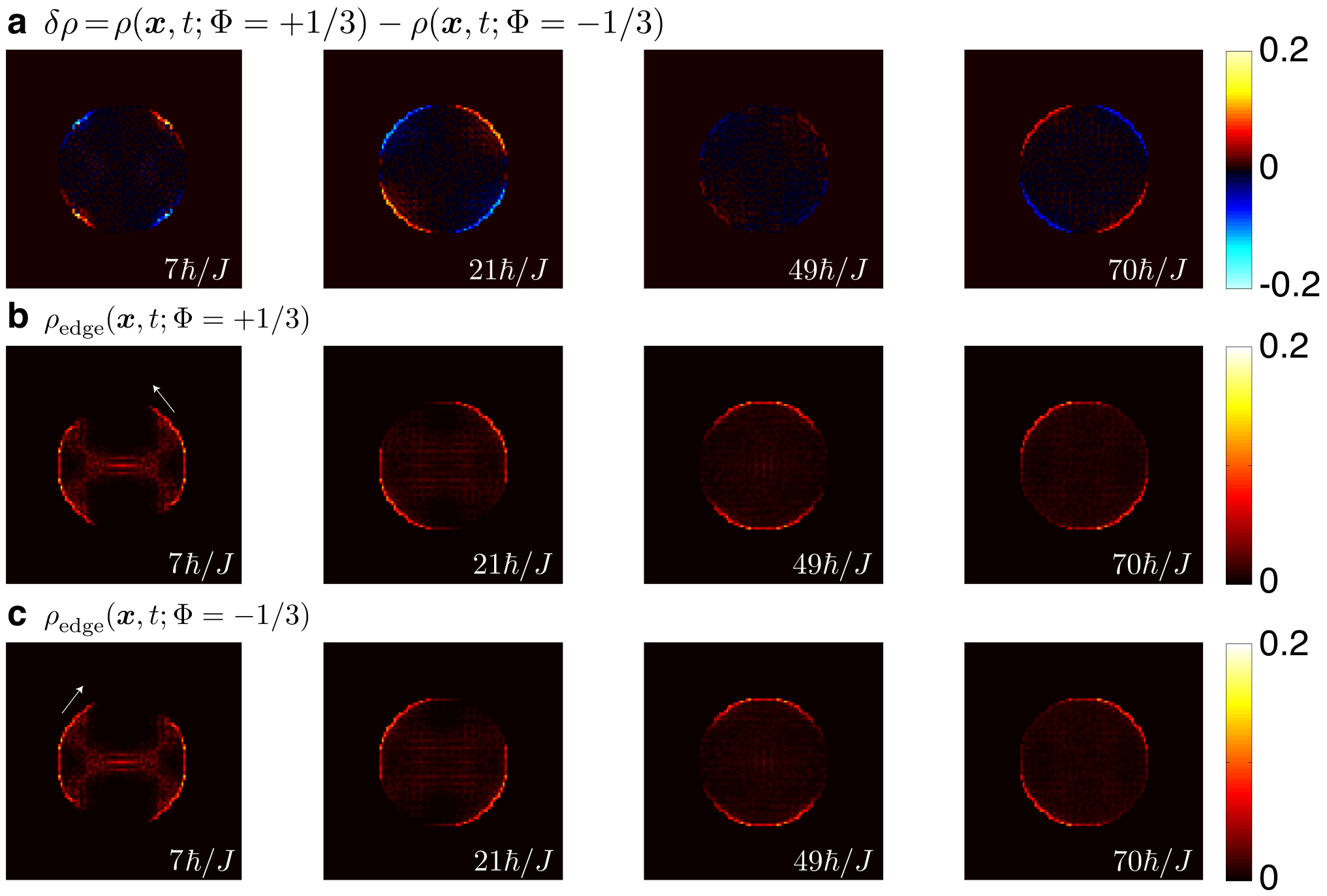
We now describe two methods for isolating the edge-states contribution from that of the bulk states, useful for systems with dispersive bulk bands. The first method consists in performing two successive experiments, using the same apparatus and parameters, but with opposite fluxes and . The difference between the two images lacks the non-chiral contribution of the bulk states and is simply given by , see Fig. 5. For our bat geometry, when the edge states have undergone a rotation of . This determines the time when the signal disappears, giving the angular velocity of the edge states. This situation is illustrated in Fig. 5 for the “dispersive” case, where we find , in good agreement with the angular velocity of the populated edge states [20, 24]. We verified that slight differences in the filling [e.g., ], for example due to finite temperature effects between the two successive experiments, or variations in the flux (e.g., and ), do not significantly affect the signal , highlighting the robustness of this method against experimental imperfections.

The second method aims to efficiently reduce the bulk dispersion by suddenly lowering the potential walls at , instead of removing them completely. This operation can be achieved in such a way that only the edge states with sufficiently high energies are allowed to propagate, while leaving the bulk states away from the holes. This “edge-filter method” can be realized by setting the Fermi energy within the first bulk gap, and then suddenly lowering the potential to the value at , where is the width of the lowest bulk band. The great efficiency of this method is presented in the Appendix C for the case .
IV Robustness of the edge states against disorder
We now investigate the robustness of the edge states motion in the presence of disorder. This perturbation, which plays a fundamental role in solid-state systems, can be engineered in optical-lattice setups, e.g., using speckle potentials [32]. We study the effects of disorder by considering a random potential , with energies uniformly distributed within the range . The results are presented in Fig. 6, for the case . We find that the chiral edge states signal remains robust for disorder strengths , where is the size of the bulk gap. Interestingly, we can still distinguish a cyclonic cloud – a signature of the edge states chirality – for values up to . The immunity of the chiral edge states against disorder, a hallmark of the quantum Hall effect, could thus be demonstrated using our cold-atom setup.

V Gaussian walls and smooth circular confinements
In the absence of walls , the edge states lying in the first bulk gap are radially localized, with a radius determined by their energy and the circular confinement. Writing the circular confinement as , we find that an edge state with energy is characterized by a localization radius
| (2) |
where is the minimum of the bulk band. This result is illustrated in Fig. 7, for , and , where the wavefunctions amplitudes are plotted as a function of the coordinate, and their corresponding energies . For an infinitely abrupt trap [27, 28], , all the edge states are located at the constant Fermi radius . Therefore, the edge states contribution to the density yields a clear circular signal, with localization length of the order of the lattice spacing . In contrast, for finite , the populated edge states are localized on different radii , leading to a broadening of the edge-state signal . For the situation illustrated in Fig. 7, this broadening is of the order for and for . Let us stress another crucial aspect of these smoothly confined QH systems, which is the fact that the angular velocity of the chiral edge states, as well as the number of available edge states within a bulk gap, highly depend on the potential’s smoothness : the angular velocity is maximized for highly abrupt confinements (), while the number is larger for smooth potentials [20, 24, 19, 31]. We numerically evaluated the angular velocity of the edge states [20, 24] for and , and we found for , for and for (and we note that the angular velocity ). Scaling to a more realistic radius , we find that the edge states, which are populated below , undergo a rotation of after a time
indicating that it is highly desirable to design a sharp circular confining trap [27, 28], to clearly observe the edge states rotating motion during reasonable experimental times .

We now investigate the density evolution for smooth confining traps and initial gaussian walls . First of all, we note that the presence of gaussian walls does not destroy the edge states lying within the first bulk gap. In this bat geometry, the edge states are localized on the outer edge delimited by , but also, on the smooth boundary delimited by the gaussian potentials. Therefore, when , the edge states behave as in Fig. 7a in the vicinity of the outer circular edge , whereas they behave similarly as in Fig. 7c in the vicinity of the gaussian walls. We point out that, in our scheme, it is the behavior of the edge states near the outer circular edge which plays an important role. Indeed, as shown in Fig. 8a, replacing the infinitely abrupt walls by gaussian potentials does not qualitatively affect the evolution of the density presented in Fig. 4a.
However, as can be anticipated from the discussion above, replacing the perfectly sharp potential by smoother confinements, , has dramatic consequences on the dynamics. In Fig. 8b, which shows the evolution of the density for , we clearly observe the broadening of the edge-state contribution , as they progressively encircle the holes. We also note the slower motion undergone by the edge states, which have a reduced angular velocity , see above. An even more dramatic situation is illustrated for the case in Fig. 8c. These results demonstrate the robustness of the edge state motion in the presence of smooth confining traps and gaussian walls, but they greatly emphasize the importance of designing sharp external confinements to improve the experimental detectability of the topological edge states.

Conclusions
In this article, we introduced a simple, yet powerful, method to image the dynamics of topological edge states in atomic systems. Our scheme shapes an atomic gas, initially prepared in a topological phase, and directly images its time evolution. By explicitly revealing the presence of propagating chiral edge modes, this method provides an unambiguous signature of topological order in the context of cold atomic gases. Importantly, we have discussed the applicability of our method under realistic experimental conditions, emphasizing the importance of using sharp confining potentials to improve the detection of the edge states signal. The schemes introduced in this work to reduce, or even eliminate, the irrelevant contribution of dispersive bulk states can be applied to a wide family of topological atomic systems, such as the promising Haldane-like optical lattice [12, 14] and fractional QH atomic gases [33, 34, 35]. Finally, our method can be directly extended to visualize the propagation of topological (spin-polarized) edge states, both in 2D [18, 36] and 3D [37], by using standard spin-dependent imaging methods [29].
Acknowledgments
We thank J. Beugnon, I. Bloch, G. Bulnes Cuetara, M. Müller, and S. Nascimbène for discussions. This work was supported by the Fonds de la Recherche Scientifique (FNRS Belgium), Agence Nationale de la Recherche (ANR) via the project AGAFON (Artificial gauge fields on neutral atoms), European Research Council (ERC) project Quantum Gauge Theories and Ultracold Atoms (QUAGATUA), the Emergences program (Ville de Paris and Université Pierre et Marie Curie), and ERC Many-Body physics in gauge fields with ultracold Yb atoms in optical lattices (ManyBo) Starting Grant. Work at Innsbruck is supported by the integrated project AQUTE, the Austrian Science Fund through Spezialforschungsbereich (SFB) F40 FOQUS, and by the Defense Advanced Research Projects Agency (DARPA) Optical Lattice Emulator (OLE) program. I.B.S. acknowledges the financial support of the National Science Foundation (NSF) through the Physics Frontier Center at Joint Quantum Institute (JQI) and the Army Research Office (ARO) with funds from both the Atomtronics Multidisciplinary University Research Initiative (MURI) and DARPA OLE Program.
References
- [1] Hasan M Z, Kane C L (2010) Colloquium: Topological insulators. Rev Mod Phys 82:3045-3067.
- [2] Qi X L, Zhang S C (2011) Topological insulators and superconductors. Rev Mod Phys 83: 1057-1110.
- [3] Thouless D J, Kohmoto M, Nightingale M P, den Nijs M (1982) Quantized Hall Conductance in a Two-Dimensional Periodic Potential. Phys Rev Lett 49: 405-408.
- [4] Kohmoto M (1989) Zero modes and the quantized Hall conductance of the two-dimensional lattice in a magnetic field. Phys Rev B 39: 11943-11949.
- [5] Hatsugai Y (1993) Chern number and edge states in the integer quantum Hall effect. Phys Rev Lett 71: 3697-3700.
- [6] Ashoori R C, Stormer H L, Pfeiffer L N, Baldwin K W, West K (1992) Edge magnetoplasmons in the time domain. Phys Rev B 45: 3894-3897.
- [7] Ji Y. et al. (2003) An electronic Mach-Zehnder interferometer Nature 422: 415-418.
- [8] Zhang Y et al. (2009) Distinct signatures for Coulomb blockade and Aharonov-Bohm interference in electronic Fabry-Perot interferometers. Phys Rev B 79: 241304.
- [9] Aidelsburger M et al. (2011) Experimental realization of strong effective magnetic fields in an optical lattice. Phys Rev Lett 107: 255301.
- [10] Dalibard J, Gerbier F, Juzeliūnas G, Öhberg P. (2011) Colloquium: Artificial gauge potentials for neutral atoms. Rev Mod Phys 83: 1523-1543.
- [11] Brantut J P, Meineke J, Stadler D, Krinner S, Esslinger T. (2012) Conduction of ultracold fermions through a mesoscopic channel. Science 337: 1069-1071.
- [12] Alba E, Fernandez-Gonzalvo X, Mur-Petit J, Pachos J K, Garcia-Ripoll J J (2011) Seeing topological order in time-of-flight measurements. Phys Rev Lett 107: 235301.
- [13] Zhao E, Bray-Ali N, Williams C, Spielman I B, Satija, I (2011) Chern numbers hiding in time-of-flight images. Phys. Rev. A 84: 063629.
- [14] Goldman N et al. (2013) Measuring topology in a laser-coupled honeycomb lattice: From Chern insulators to topological semi-metals. New J Phys 15:013025.
- [15] Price H M, Cooper N R (2012) Mapping the Berry curvature from semiclassical dynamics in optical lattices. Phys. Rev. A. 85: 033620.
- [16] Umucalilar R O, Zhai H, Oktel M. Ö. (2008) Trapped Fermi gases in rotating optical lattices: Realization and detection of the topological Hofstadter insulator. Phys Rev Lett 100: 070402.
- [17] Scarola V W, Das Sarma S (2007) Edge transport in 2D cold atom optical lattices. Phys Rev Lett 98: 210403.
- [18] Goldman N et al. (2010) Realistic time-reversal invariant topological insulators with neutral atoms. Phys Rev Lett 105: 255302.
- [19] Stanescu T D, Galitski V, Das Sarma S (2010) Topological states in two-dimensional optical lattices. Phys Rev A 82: 013608.
- [20] Goldman N, Beugnon J, Gerbier F (2012) Detecting chiral edge states in the Hofstadter optical lattice. Phys Rev Lett 108: 255303.
- [21] Kraus C V, Diehl S, Zoller P, Baranov M A (2012) Preparing and probing atomic Majorana fermions and topological order in optical lattices. New J Phys 14: 113036.
- [22] Killi M, Paramekanti A (2012) Use of quantum quenches to probe the equilibrium current patterns of ultracold atoms in an optical lattice. Phys. Rev. A 85: 061606(R).
- [23] Papp S B et al. (2008) Bragg spectroscopy of a strongly interacting 85Rb Bose-Einstein condensate. Phys. Rev. Lett. 101: 135301.
- [24] Goldman N, Beugnon J, Gerbier F (2013) Identifying topological edge states in 2D optical lattices using light scattering. Eur Phys J Special Topics 217:135Ð152.
- [25] Jaksch D, Zoller P (2003) Creation of effective magnetic fields in optical lattices: the Hofstadter butterfly for cold neutral atoms. New J Phys 5: 56.
- [26] Gerbier F, Dalibard J. (2010) Gauge fields for ultracold atoms in optical superlattices. New J Phys 12: 033007.
- [27] Meyrath T P, Schreck F, Hanssen J L, Chuu C S, Raizen M G (2005) Bose-Einstein condensate in a box. Phys Rev A 71: 041604(R).
- [28] Gaunt A L, Schmidutz T F, Gotlibovych I, Smith R P and Hadzibabic Z (2012) Bose-Einstein condensation of atoms in a uniform potential. arXiv:1212.4453.
- [29] Weitenberg C et al. (2011) Single-spin addressing in an atomic Mott insulator. Nature 471: 319-324.
- [30] Hofstadter D R (1976) Energy levels and wave functions of Bloch electrons in rational and irrational magnetic fields. Phys Rev B 14: 2239-2249.
- [31] Buchhold M, Cocks D, Hofstetter W (2012) Effects of smooth boundaries on topological edge modes in optical lattices. Phys Rev A 85: 63614.
- [32] Sanchez-Palencia L, Lewenstein M (2010) Disordered quantum gases under control. Nat Phys 6: 87-95.
- [33] Sorensen A S, Demler E, Lukin M D (2005) Fractional quantum Hall states of atoms in optical lattices. Phys Rev Lett 94: 086803.
- [34] Cooper N R (2008) Rapidly rotating atomic gases. Adv Phys 57: 539-616.
- [35] Graß T, Juliá-Díaz B, Lewenstein M (2012) Quasihole dynamics as a detection tool for quantum Hall phases. Phys Rev A 86: 053629.
- [36] Béri B, Cooper N R (2011) topological insulators in ultracold atomic gases. Phys. Rev. Lett. 107: 145301.
- [37] Bermudez A et al. (2010) Wilson fermions and axion electrodynamics in optical lattices. Phys. Rev. Lett. 105: 190404.
Appendix A The time evolution, observable quantities and states population
The system is prepared in the ground-state of the initial Hamiltonian,
| (3) |
where the potential describes the walls initially present in the trap (see main text), and where is given by Eq. (1). We denote the number of available sites before and after removing the walls by and , respectively, and we define the ratio . When , the total number of sites within the trap is approximatively given by the area , while the outer circular edge contains about lattice sites. The holes in the density created by correspond to vacant sites, leading to the large ratio . For , the system initially contains sites and the number of sites delimiting the edge of the bat is sites. Thus, the spacious holes used in our calculations lead to a large edge/bulk ratio. For , and initially setting the Fermi energy in the lowest bulk gap, leads to the filling factor . After removing the walls , the filling factor is reduced to the smaller value .
The groundstate of Hamiltonian (3) is written as
| (4) |
where the operator creates a particle in the single-particle state , with energy located below the Fermi energy . Here represents the complete set of single-particle eigenstates and eigenvalues satisfying the stationary Schrödinger equation
| (5) |
We are interested in the time evolution of the spatial density after removing the walls at . The evolution of the single-particle states is then entirely governed by the Hamiltonian . It is therefore convenient to introduce the eigenstates and eigenvalues corresponding to the Hamiltonian ,
| (6) |
We then define as the time evolution of the initial state according to the Hamiltonian ,
| (7) |
The spatial density at time is given by
| (8) |
namely, the particle density is entirely governed by the time-evolution of the initially occupied single-particle states. The time evolution of the atomic cloud, after releasing the walls at , can therefore be numerically evaluated through a direct diagonalization of the Hamiltonians and . In our study, a crucial aspect consists in identifying the regimes for which the edge states propagating around the initially forbidden regions provide a clear signal, which is not perturbed by the many bulk states. It is therefore desirable to separately evaluate the contributions of the initially populated bulk and edge states. We introduce the corresponding quantities
where the sum is restrained to the populated edge states with energies located within the bulk gap.
In this study, the time evolution is chosen to be entirely dictated by the Hamiltonian , and thus, it is non-dissipative: after releasing the walls, the total energy of the system is constant and is given by
| (9) |
where we considered the approximation , which is valid for sufficiently abrupt. For example, in the situation illustrated in Fig. 4, the energy released after removing the walls is about . Therefore, in our calculations, the many-body state never reaches the ground state of the final Hamiltonian , with energy
| (10) |
This final ground state, which differs from the initially prepared ground state in Eq. (4), is expressed as
| (11) |
where creates a particle in the single-particle state , with energy . Here, is the total number of particles in the system, which is supposed to be constant (see Figs. Aa-b). In our non-dissipative framework, the probability of finding a particle in the eigenstate is constant and inferior to one, as it is simply given by
| (12) |
The populations are illustrated as a histogram in Fig. Ac, for the case and . We find that when the Fermi energy is initially set within the first bulk gap, the population of high-energy dispersive bulk bands is highly limited during the evolution, which guarantees a clear spatial separation of the bulk and edge signal in this “topological quasi-flat band” configuration. The efficiency with which the initial edge modes project to the final edge modes is further shown in Fig. B, indicating the success of our scheme. For the situation illustrated in Figs. A-B, we find that the number of populated edge states , where is the number of populated edge states before removing the walls (see main text). This result is in agreement with the fact that the edge delimited by the bat contains sites, where is the number of sites delimited by the external circular confinement.
In the main text, we discuss the non-dissipative evolution of the atomic cloud after releasing the walls , neglecting thermalization processes. However, it is instructive to estimate the energy loss that would be required to reach the ground state , namely . We propose to evaluate this energy difference for a configuration which is particularly relevant for our work (see main text), namely, a system exhibiting large initial holes and a flat (dispersionless) lowest bulk band. In the following, we set the energy of the lowest bulk band equal to zero. The energy difference will generally be large in this “large hole/flat band” situation, since many bulk states become available in the lowest energy band after removing the walls, namely [see Figs. Aa-b and below]. For this configuration, which is particularly suitable for visualizing the edge states encircling the holes, the energy difference is thus approximatively given by
| (13) |
where we considered the Fermi energy to be located inside the first bulk gap [see Fig. Aa-b]. For large holes , the final filling factor such that the lowest bulk band will only be partially occupied when reaching the ground state , and thus . From a rough geometric argument, we expect about available edge states in the lowest bulk gap of the initial system. Approximating the edge-state branch as being linear inside the whole gap , we find
| (14) |
which corresponds to an energy difference in the case and (see main text). In a typical experiment, , which would require an important energy loss to reach the ground state . We verified that the estimated energy difference in Eq. (14) is in good agreement with a direct numerical evaluation of Eq. (13), for the system illustrated in Fig. 4 (i.e., , and ). As illustrated in Fig. Ab, the ground state generally consists in a partially occupied bulk band, which indicates that the edge states will no longer be populated if the system relaxes to the ground state . Therefore, our scheme requires that the system remains in an excited state during the time evolution, namely, that dissipation should be limited.

Appendix B The opposite-flux method for dispersive bulk bands
In this Section, we discuss how the difference , obtained from two successive measurements with opposite magnetic fluxes, is related to the edge states contributions . We show in Fig. Ca, the evolution of for the dispersive case , which clearly indicates that the contributions from the bulk vanish from the signal at all times . Accordingly, . To clarify the evolution of this signal, which has non-vanishing values in the vicinity of the Fermi radius , we show the chiral evolution of the edge states contribution in Figs. Cb-c. At small times, the overlap between the two contributions decreases in time, leading to a progressive broadening of the signal along the 1D circular edge. Then, after reaching a rotation of , the overlap increases, and eventually leads to a vanishing of the signal when the edge states have undergone a rotation of , where . In Fig. C, this happens at time , indicating that the edge states angular velocity is for . The opposite-flux method therefore offers a general technique for emphasizing the existence of chiral edge states in dispersive systems, and also, for evaluating their characteristic angular velocity.
We verified that a slight difference in the filling, , or variations in the flux, and , does not significantly affect the signal shown in Fig. C a, highlighting the robustness of this method against possible experimental imperfections.
Appendix C The edge-filter method for dispersive bulk bands
Another strategy consists in allowing the edge states to propagate at , while forbidding the bulk states to penetrate the regions initially occupied by the holes. This can be achieved by suddenly lowering the additional potential walls to some intermediate value , instead of removing them completely at . This “edge-filter” scheme is illustrated in Fig. Da, for the dispersive case . By suddenly lowering the walls potential to the value , where is the width of the lowest bulk band, we limit the undesired filling of the holes by the bulk states at times . In contrast, the populated edge states with energy , where is the minimum of the bulk band, are allowed to propagate around the holes without being spoiled by the bulk. The resulting time evolution of the density , presented in Fig. Db, shows a clear propagation of the edge states around the holes. Experimentally, this method offers an efficient method to isolate the edge states contribution from the spoiling bulk background, but it necessitates a very precise control over the potential strength .

Appendix D Sensitivity to imperfect filling
Our general scheme is based on the possibility of preparing a QH atomic state, which can be achieved by generating a magnetic flux in the lattice and filling the lowest bulk band completely. In other words, one has to tune the total number of particles in such a way that the Fermi energy lies within the lowest bulk gap. According to the topological nature of the lowest bulk band, one is then guaranteed that topological edge states are populated. In practice, the total number of particles (and the corresponding Fermi energy ) can be tuned with a great precision in cold-atom experiments. However, it is instructive to test the robustness of our method against inexact filling effects, in particular, for the dispersionless case . We remind that in this configuration, the clear separation of the bulk and edge states contributions to the density relies on the fact that the bulk states are dispersionless (they are described by a quasi-flat band). Here, we show that this picture holds even when the second (dispersive) bulk band is dramatically filled, see Fig. E. From this result, we find that the high-energy bulk states contribute in a non-chiral manner to the density evolution, see Fig. E, and that their dispersive motion is slow compared to the edge states propagation along the circular boundary. In particular, this shows that the chiral picture drawn by the density , and which will be imaged in an experiment, can unambiguously be attributed to the populated edge states. We conclude that the edge-state signal obtained for the interesting case remains clear and detectable, as long as sufficiently many edge states are initially populated. In particular, this indicates that our scheme is robust at finite temperature , as long as it remains small compared to the gap’s width , in order to insure a sufficiently large edge-state population.

Appendix E The holes geometry and size effects
Our setup illustrated in Fig. 1 features two large repulsive potentials, which create the initial bat geometry. These holes are chosen to be created by infinitely abrupt walls , which are delimited by the two ellipses
where the coordinates at the center of the trap. This choice is motivated by the fact that these walls coincide (up to first order) with the external circular wall of radius , in the vicinity of the poles located at . Note that in the following of this discussion, we consider that with .

The geometry produced by these potentials is particularly suitable to emphasize the edge states motion at time , as they encircle the regions initially surrounded by the elliptical walls. However, in this exotic geometry, the large holes correspond to a massive distortion of the standard circular system. It is thus interesting to study the validity of our method, as we progressively reduce the size of the holes. Here, we demonstrate that our scheme still shows a clear manifestation of the edge states, even in the limit where the walls only represent a small perturbation of the system, in the vicinity of its circular boundary. To analyze this, we propose to calculate the time evolution of the density after removing the elliptical walls delimited by the more general equations
| (15) |
which can be made arbitrarily small (), while maintaining the smooth contact with at the poles. The results are shown in Fig. F for the flat-band configuration previously studied in Fig. 4 (for ), but with smaller initial holes . This picture emphasizes the fact that our scheme still allows to detect the chiral motion of the edge states, in the limit of small perturbative walls . However, we stress that it is crucial to prohibit any broadening of the edge state signal in the perturbative regime , which necessarily requires the use of an extremely abrupt external potential with . Moreover, considering smaller holes also demands to further reduce the bulk dispersion, which can be achieved by considering the quasi-flat-band configuration , see Fig. F, or by exploiting the “opposite-flux” or “edge-filter” methods.
Another relevant configuration is obtained by replacing the constraining potentials by a spacious wall that initially confines the entire atomic cloud to a small region located in the vicinity of the circular edge delimited by , see Fig. G. After releasing the wall at time , the edge states propagate along the circular edge delimited by , while the bulk states evolve towards the center of the trap. This strategy, which largely improves the edge/bulk ratio, is particularly efficient for dispersionless systems (e.g. ).

Appendix F Time evolution of a trivial insulating phase
The chiral motion of the edge states shown in Figs. 3 and 4 is a signature of the non-trivial Chern number (see main text). As illustrated in Fig. 5, reversing the sign of the magnetic flux leads to an opposite chirality, in agreement with the fact that the Chern number also changes its sign under the transformation. Here, we further demonstrate that the edge-states motion, visible in the time-evolving density , can be unambiguously attributed to the non-triviality of the Chern number. We consider the same system, but in a configuration characterized by a trivial Chern number . This configuration is produced in the following way: (i) We set the flux to the value , which leads to a gapless bulk energy spectrum displaying two Dirac cones. (ii) We add a staggered potential along both spatial directions, with alternating on-site energies , which opens a bulk gap around . This gap is trivial in the sense that the lowest band is associated with a zero Chern number , and therefore, edge states are unexpected in this configuration. We represent in Fig. H the time-evolving density, obtained by initially setting the Fermi energy within the trivial gap. This figure H, which is to be compared with Fig. 3, shows (i) the non-chiral dynamics of the bulk states initially occupying the lowest band, and (ii) the absence of chiral edge states.
