FOURIER DOMAIN BEAMFORMING FOR MEDICAL ULTRASOUND
Abstract
Sonography techniques use multiple transducer elements for tissue visualization. Signals detected at each element are sampled prior to digital beamforming. The required sampling rates are up to 4 times the Nyquist rate of the signal and result in considerable amount of data, that needs to be stored and processed. A developed technique, based on the finite rate of innovation model, compressed sensing (CS) and Xampling ideas, allows to reduce the number of samples needed to reconstruct an image comprised of strong reflectors. A significant drawback of this method is its inability to treat speckle, which is of significant importance in medical imaging. Here we build on previous work and show explicitly how to perform beamforming in the Fourier domain. Beamforming in frequency exploits the low bandwidth of the beamformed signal and allows to bypass the oversampling dictated by digital implementation of beamforming in time. We show that this allows to obtain the same beamformed image as in standard beamforming but from far fewer samples. Finally, we present an analysis based CS-technique that allows for further reduction in sampling rate, using only a portion of the beamformed signal’s bandwidth, namely, sampling the signal at sub-Nyquist rates. We demonstrate our methods on in vivo cardiac ultrasound data and show that reductions up to 1/25 over standard beamforming rates are possible.
Index Terms:
Array Processing, Beamforming, Compressed Sensing, Speckle, UltrasoundDept. of Electrical Engineering
Haifa 32000, Israel
1 Introduction
Diagnostic ultrasound has been used for decades to visualize body structures. The overall imaging process is described as follows: An energy pulse is transmitted along a narrow beam. During its propagation echoes are scattered by acoustic impedance perturbations in the tissue, and detected by the elements of the transducer. Collected data are sampled and digitally processed in a way referred to as beamforming, which results in signal-to-noise ratio (SNR) enhancement. Such a beamformed signal forms a line in the image.
According to the classic Shannon-Nyquist theorem [1], the sampling rate at each transducer element should be at least twice the bandwidth of the detected signal. Rates up to 4 times the Nyquist rate are required in order to avoid artifacts caused by digital implementation of beamforming [2]. Taking into account the number of transducer elements and the number of lines in an image, the amount of sampled data that needs to be digitally processed is enormous, motivating methods to reduce sampling rates. Reduction of processing rate is possible within the classical sampling framework by exploiting the fact that the signal is modulated onto a carrier and occupies only a portion of its entire baseband bandwidth. Accordingly, modern systems digitally down-sample the data at the system’s front-end. However, this does not change the sampling rate since demodulation takes place in the digital domain. In addition, the processing rate may be reduced up to 1/4 of the sampling rate, but the signal becomes complex in this setup, and the number of samples effectively is only twice smaller.
A different approach to sampling rate reduction is introduced in [3]. Tur et. al. regard the ultrasound signal detected by each receiver within the framework of finite rate of innovation (FRI) [4], modeling it as replicas of a known pulse-shape, caused by scattering of the transmitted pulse from reflectors, located along the transmitted beam. Such an FRI signal is fully described by parameters, corresponding to the replica’s delays and amplitudes. These parameters can be extracted from a small set of the signal’s Fourier series coefficients. A mechanism, referred to as Xampling, derived in [5], extracts such a set of coefficients from real-valued samples. This work is continued in [6], where Wagner et. al. introduce a generalized scheme, referred to as compressed beamforming, which allows to compute the Fourier series coefficients of the beamformed signal from the low-rate samples of signals detected at each element. The problem of reconstruction of the beamformed signal from a small number of its Fourier series coefficients is solved via a compressed sensing (CS) technique, while assuming a small number of replicas. This approach allows to reconstruct an image comprised of macroscopic perturbations, but cannot treat the speckle, which is of significant importance in medical imaging.
In our work we extend the notion of compressed beamforming to beamforming in frequency and show explicitly how to perform it. Beamforming in frequency exploits the low bandwidth of the beamformed signal and allows to bypass the oversampling dictated by the digital implementation of beamforming in time. We reconstruct the beamformed signal perfectly with a simple inverse discrete Fourier transform (IDFT) from a small set of its discrete Fourier transform (DFT) coefficients, that are computed from low-rate samples of individual signals. We show that beamforming in frequency allows to preserve the integrity of an image with 7 fold reduction in the number of samples used for its reconstruction.
Finally, we introduce an analysis based CS-technique [7] for signal reconstruction using only a portion of the beamformed signal’s bandwidth. We demonstrate our methods on in vivo cardiac ultrasound data and show that reductions of up to 1/25 of beamforming rate and up to 1/3 of Nyquist rate are possible. The proposed reconstruction method outperforms the classic synthesis CS approach used in [6], when the same number of samples is used.
The rest of the paper is organized as follows: in Section 2, we review beamforming in time. In Section 3 we describe the principles of frequency domain beamforming. In Section 4 we describe how the reduction in sampling rate is achieved. In Section 5 we discuss two possible CS approaches to signal reconstruction.
2 Beamforming in time
Most modern imaging systems use multiple transducer elements to transmit and receive acoustic pulses. Appropriate processing of the signals detected by the individual array elements allows to enhance the quality of the resulting image. The most commonly used technique, referred to as beamforming, increases SNR by averaging the individual signals after their alignment with appropriate time-delays. We begin by describing the beamforming process which takes place in a typical B-mode imaging cycle. Our presentation is based mainly on [8] and [6].
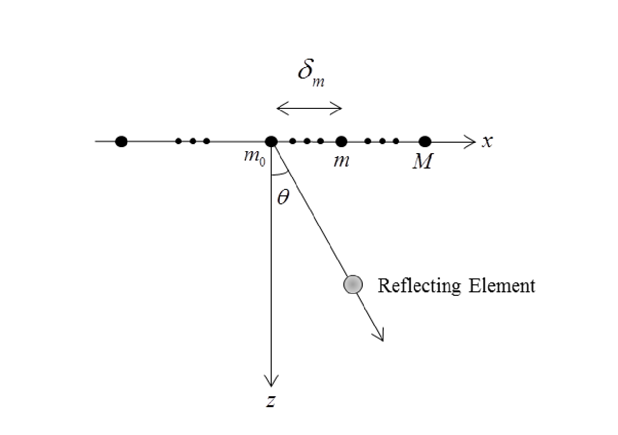
Consider an array comprised of transceiver elements aligned along the axis, as illustrated in Fig. 1. The reference element is set at the origin and the distance to the -th element is denoted by . The image cycle begins at , when the array transmits an energy pulse in the direction . The pulse propagates trough the tissue at speed , and at time its coordinates are . A potential point reflector located at this position scatters the energy, such that the echo is detected by all array elements at a time depending on their locations. Denote by the signal detected by the -th element and by the time of detection. It is readily seen that:
| (1) |
where is the distance traveled by the reflection. Beamforming involves averaging the signals detected by multiple receivers while compensating the differences in detection time.
Using (1), the detection time at is since . Applying an appropriate delay to , such that the resulting signal satisfies , we can align the reflection detected by the -th receiver with the one detected at . Denoting and using (1), the following aligned signal is obtained:
| (2) | ||||
The beamformed signal may now be derived by averaging the aligned signals:
| (3) |
Ultrasound systems perform the beamforming process defined in (3) in the digital domain, implying that the analog signals detected at the receiver elements are first sampled. Rates up to 4 times the Nyquist rate, dictated by the bandwidth of the individual signal, are required in order to improve the system’s beamforming resolution and to avoid artifacts caused by digital implementation. From now on we will denote this sampling rate as the beamforming sampling rate .
To conclude this section we evaluate the number of samples taken at each transducer element. Our evaluation is based on the imaging setup used to acquire in vivo cardiac data. The acquisition was performed with a GE breadboard ultrasonic scanner of 64 acquisition channels. The radiated depth cm and the speed of the sound m/sec yield a signal of duration sec. The acquired signal is characterized by a narrow bandpass bandwidth of MHz, centered at the carrier frequency MHz, leading to a beamforming rate of MHz and real-valued samples.
3 Beamforming in frequency
We now show that beamforming can be performed equivalently in the frequency domain, leading to substantial reduction in the number of samples, needed to obtain the same image quality.
We extend the notion of compressed beamforming, introduced in [6], to beamforming in frequency and show that a linear combination of the DFT coefficients of the individual signals, sampled at the beamforming rate , yields the DFT coefficients of the beamformed signal, sampled at the same rate. We follow the steps in [6] and start from the computation of the Fourier series coefficients of the beamformed signal .
The support of is limited to , with defined by the transmitted pulse penetration depth. Its Fourier series coefficients are given by:
| (4) |
Plugging (3) into (4), it can be shown that
| (5) |
where are the Fourier coefficients of . These coefficients can be written as
| (6) |
with
| (7) | ||||
where , and is the indicator function.
Our next step is to substitute by its Fourier series coefficients. Denoting the -th Fourier coefficient by and using (7) we can rewrite (6) as follows:
| (8) |
where are the Fourier coefficients of with respect to . According to Proposition 1 in [6], can be approximated sufficiently well when we replace the infinite summation in (8) by the finite one:
| (9) |
The set is defined according to the decay properties of . Equations (5) and (9) provide a relationship between the Fourier series coefficients of the beamformed and the individual signals. Denote by the number of samples in each signal. Since all signals are sampled at a rate which is higher than their Nyquist rate, the relation between the DFT of length and the Fourier series coefficients is given by:
| (10) |
where and denote the DFT coefficients of the beamformed and individual signals respectively. Plugging (10) into (5) and (8), we get the desired relation:
| (11) |
Note that in order to calculate an arbitrary set of DFT coefficients of the beamformed signal, we need DFT coefficients of each one of the individual signals.
Applying an IDFT on , we obtain the beamformed signal. We can now proceed to standard image generation steps which include log-compression and interpolation. To demonstrate the equivalence of beamforming in time and frequency, we applied both methods on in vivo cardiac data obtained as explained in Section 2, yielding the images shown in Fig. 2. As can be seen, both images are identical.

(a)

(b)
4 Rate Reduction by Beamforming in Frequency
In the previous section we showed the equivalence of beamforming in time and frequency. We next demonstrate that beamforming in frequency allows to reduce the required number of samples of the individual signals. To this end we consider two questions: 1) how many DFT coefficients of the beamformed signal do we need for its perfect reconstruction; 2) how many samples of the individual signals should be taken in order to compute these DFT coefficients?
4.1 Parametric representation
We begin by answering the first question using a parametric model for the beamformed signal. According to [3, 6], the beamformed signal can be modeled as a sum of a small number of replicas of the known transmitter pulse with unknowns amplitudes and delays:
| (12) |
where is the transmitted pulse-shape, is the number of scattering elements in direction , are the unknown amplitudes of the reflections and denote the times at which the reflection from the -th element arrived at the reference receiver . Sampling both sides of (12) at rate and quantizing the unknown delays with quantization step , such that , we can rewrite (12) as follows:
| (13) |
where
Calculating the DFT using (13):
| (16) |
where is the DFT coefficient of .
The transmitted pulse may be modeled as a narrowband waveform, , modulated by a carrier at frequency : . When such a pulse is sampled at rate , most of its DFT coefficients are zero, as shown in Fig. 3. Obviously, (16) implies that the only non-zero DFT coefficients are in the bandwidth of the transmitted pulse. This allows us to exploit the low bandwidth of the beamformed signal and calculate only non-zero DFT coefficients. Since is real, its DFT coefficients are symmetric, thus we only need to know half of the overall non-zero elements. Denote the set of non-zero DFT coefficients by . In typical cardiac imaging the bandwidth of is equal to MHz, the modulation frequency MHz, and the sampling rate MHz, leading to . Once these coefficients are known, we can reconstruct by padding the elements of with an appropriate number of zeros and performing an IDFT. Hence, we have shown that the number of DFT coefficients of the beamformed signal required for its perfect reconstruction is the cardinality of the set . This number is only of the overall number of DFT coefficients of beamformed signal dictated by .

4.2 Reduced rate sampling
We now address the second question: how many samples of the individual signals should be taken in order to compute the set of non-zero DFT coefficients ?
As shown in Section 3, we need to know a set of the DFT coefficients of each individual signal in order to compute a set of the DFT coefficients of the beamformed signal. The experimental results show that in ultrasound imaging scenario, . According to (10), we equivalently seek the same set of Fourier series coefficients of each individual signal. The above problem is addressed in [6]. A mechanism, proposed there, allows to obtain a set of Fourier coefficients of the beamformed signal from samples of each of the individual signals, filtered with an appropriate kernel. Namely, the number of the samples taken from the individual signal is . For the setup mentioned in Subsection 4.1, , implying that in the worst case we need only samples of the individual signal, while for beamforming in time domain we need samples as shown in Section 2. This allows us to achieve 7-fold reduction in sampling rate without compromising image quality. The images, created by these two techniques, shown in Fig. 4, are identical.
(a)

(b)
5 Further Reduction via CS
We showed that it is possible to reconstruct a beamformed signal perfectly from the set of its non-zero DFT coefficients, computed from a small number of samples of the individual signals. We show next that further reduction in sampling rate is possible, when taking only a subset , , of DFT coefficients of the beamformed signal.
Defining a -length vector with -th entry , we can rewrite (16) in matrix form:
| (17) |
where is a matrix formed by taking the set of rows from an DFT matrix, and vector is of length with -th entry . Since from now on only subset is given, define an -length vector with -th entry and rewrite (17) as follows:
| (18) |
where is measurement matrix which picks the subset of rows from , implying that is matrix formed by taking the set of rows from an DFT matrix.This property of will be used below.
5.1 Synthesis approach
Since from (13) the signal of interest is completely defined by the unknown delays and amplitudes, a possible approach is to extract those values from the available set of DFT coefficients. Equation (18) can be viewed from a CS perspective, when we assume that the number of scatterers is small, since according to (4.1) it implies that the vector is sparse. Hence (18) has the form of a classic sparse synthesis model [9], where vector has a sparse representation in . The goal is to reconstruct an -sparse vector from its projection onto a subset of orthogonal vectors given by the rows of matrix . With an appropriate choice of and subset of fourier coefficients , such a problem can be solved using CS methodology, including optimization and greedy algorithms. Indeed, in [6], orthogonal matching pursuit (OMP) [10] shows sufficiently good performance.
The synthesis approach has a significant drawback. The assumption of a small number of reflecting elements , forces us to treat only the strong reflectors located in direction . In such a setup we essentially loose all the weak reflectors that appear as speckle, namely, granular pattern that can be seen in Fig. 2, and carry important information in medical imaging.
5.2 Analysis approach
To avoid loss of speckle information, imposed by the assumption of sparsity, we propose using an analysis approach [7]. In this methodology we aim to reconstruct the set from its subset , while assuming that the analyzed vector is compressible. The analysis approach can be translated into the optimization problem:
| (19) |
According to Theorem 1.4 in [7], the solution to (19) is very accurate, if the measurement matrix satisfies the restricted isometry property adapted to (D-RIP) and the elements of decay rapidly. As we mentioned before, is a partial DFT matrix, therefore, according to results in [7], satisfies the D-RIP.
A typical beamformed ultrasound signal is comprised of a relatively small number of strong reflections and a bunch of much weaker scattered echoes. It is, therefore, natural to assume that is compressible, implying that has a compressible expansion in . Since is a partial DFT matrix, its Gram matrix is nearly diagonal, implying that is also compressible [7] and satisfies the decay requirement.
To demonstrate the proposed method, a subset of Fourier coefficients corresponding to the central frequency samples in the bandwidth of the transmitted pulse were chosen. To calculate we need at most samples per individual signal, implying 25 fold reduction in sampling rate. The result is shown in Fig. 5 (a). To compare the proposed solution with the previously developed OMP based method [6], the same subset was used to reconstruct the beamformed signal assuming strong reflectors in each direction . The resulting image is shown in Fig. 5 (b).

(a)

(b)
References
- [1] C. E. Shannon, “Communication in the presence of noise,” Proceedings of the IRE, vol. 37, no. 1, pp. 10–21, 1949.
- [2] T. L. Szabo, Diagnostic Ultrasound Imaging: Inside Out, Academic Press, 2004.
- [3] R. Tur, Y.C. Eldar, and Z. Friedman, “Innovation rate sampling of pulse streams with application to ultrasound imaging,” Signal Processing, IEEE Transactions on, vol. 59, no. 4, pp. 1827–1842, 2011.
- [4] M. Vetterli, P. Marziliano, and T. Blu, “Sampling signals with finite rate of innovation,” IEEE Transactions on Signal Processing, vol. 50, no. 6, pp. 1417–1428, 2002.
- [5] K. Gedalyahu, R. Tur, and Y. C. Eldar, “Multichannel sampling of pulse streams at the rate of innovation,” IEEE Transactions on Signal Processing, vol. 59, no. 4, pp. 1491–1504, 2011.
- [6] N. Wagner, Y. C. Eldar, and Z. Friedman, “Compressed beamforming in ultrasound imaging,” IEEE Transactions on Signal Processing, vol. 60, no. 9, pp. 4643–4657, 2012.
- [7] E. J. Candes, Y. C. Eldar, D. Needell, and P. Randall, “Compressed sensing with coherent and redundant dictionaries,” Applied and Computational Harmonic Analysis, vol. 31, no. 1, pp. 59–73, 2011.
- [8] J. A. Jensen, “Linear description of ultrasound imaging systems,” Notes for the International Summer School on Advanced Ultrasound Imaging, Technical University of Denmark July, vol. 5, 1999.
- [9] Y. C. Eldar and G. Kutyniok, “Compressed sensing: Theory and applications,” New York: Cambridge Univ. Press, vol. 20, pp. 12, 2012.
- [10] J. A. Tropp and A. C. Gilbert, “Signal recovery from random measurements via orthogonal matching pursuit,” IEEE Transactions on Information Theory, vol. 53, no. 12, pp. 4655–4666, 2007.