Growing Random Geometric Graph Models of Super-linear Scaling Law
Abstract
Recent researches on complex systems highlighted the so-called super-linear growth phenomenon. As the system size measured as population in cities or active users in online communities increases, the total activities measured as GDP or number of new patents, crimes in cities generated by these people also increases but in a faster rate. This accelerating growth phenomenon can be well described by a super-linear power law (). However, the explanation on this phenomenon is still lack. In this paper, we propose a modeling framework called growing random geometric models to explain the super-linear relationship. A growing network is constructed on an abstract geometric space. The new coming node can only survive if it just locates on an appropriate place in the space where other nodes exist, then new edges are connected with the adjacent nodes whose number is determined by the density of existing nodes. Thus the total number of edges can grow with the number of nodes in a faster speed exactly following the super-linear power law. The models cannot only reproduce a lot of observed phenomena in complex networks, e.g., scale-free degree distribution and asymptotically size-invariant clustering coefficient, but also resemble the known patterns of cities, such as fractal growing, area-population and diversity-population scaling relations, etc. Strikingly, only one important parameter, the dimension of the geometric space, can really influence the super-linear growth exponent .
pacs
89.75.-k,89.75.DaI Introduction
The super-linear phenomenon is described as a scaling relation,
| (1) |
and may have different representations in different systems. In urban systems, for example, represents GDP, R&D investments, crimes or the number of new patents, and represents the population[1, 2, 3, 4]. In online communities, is the total number of activities (tags, blogs) generated by the users, and is the total number of active users (who at least generate one activity)[5]. In language, is the total number of words in an article, is the number of distinct words in the same article[6, 7]. In equation 1, is an exponent to describe the relative speed of respective to . A large number of empirical studies reported that is always falling into the interval . For example, [5] pointed out s are for different online communities. [1] finds s are for cities in different countries. However, the exponent for the relationship of population and GDP can approach to if the scale of the system is large and interactions among people are weak. For example, [8] found that the exponent is almost for countries. According to our unpublished results, the scaling relationship is almost linear for provinces and states. So far, we know the equation 1 holds for a large number of different systems, but the exponents are always different system by system. While, the next question is what is the underlying mechanism of this remarkable phenomenon?
There are already some studies trying to explain the super-linear growth phenomenon. For instance, Arbesman et al. tried to attribute the super-linear phenomenon to the properties of the interaction network[9], but their model takes several assumptions on the network which are hardly to find the correspondence in the real systems. While [5, 7] tried to link the universal patterns in distributions (e.g. DGBD distribution in [5] and Zipf law in [7]) to the super-linear growth pattern by large number of empirical data. Despite a strong connection between size-dependent distributions and super-linear growth is revealed [5], the underlying mechanisms are still unknown since size-dependent distribution and super-linear growth actually are the two different expressions for the same law[5].
In the network community, researchers have found many empirical networks are of a so-called accelerating growth phenomenon[10, 11] which also states the power law relationship between the number of edges () and the number of nodes (), but they didn’t try to explain this fact. Leskovec et al. [12] re-found the accelerating growth pattern and re-name it as the densification phenomenon. He tried to build a forest fire model to understand its origin[12]. But due to the complexity of this model, he later developed a totaly new one called kronecker graph model. As claimed in [13], densification phenomenon is a mathematical property of kronecker products. Although it succeeds to fit many empirical network data, the explanations and real life grounding are still lack. Also, in kronecker graph model, the intercept of the power law relation between number of nodes and edges, i.e., in equation 1 must be 1. This strong assumption is hardly supported by empirical data. However, these studies make us clear that the super-linear growth pattern widely existing in various systems can be discussed on a network background. Recently, by analyzing the data of cell-phone communication networks in different cities, Schlapfer et al.[14] found the accelerating growth exponent is of the same value as the super-linear growth exponent of cities and the clustering coefficients in these networks are size invariant. This coefficient almost determines the super-linear growth exponents[14]. Therefore, as the size of the network increases, the clustering coefficient must keep unchanged so that the accelerating growth or densification pattern as a systemic results can emerge. However, their model cannot answer what is the origin of the size-invariant clustering coefficient, so the super-linear growth puzzle also remained unsolved. More recently, Bettencourt developed a network model to explain the origin of the super-linear growth in urban systems[15]. Although this model can fit the empirical data of cities very exactly, it is complicated and depends on a set of assumptions which are hardly tested.
Despite several models have been presented to explain the super-linear growth scaling law, we still cannot find one simple model with minimum parameters while can reproduce as many as possible patterns observed in empirical systems. In this paper, we propose a new growing network modeling framework in geometric space called growing random geometric models to explain the super-linear phenomenon. It uses very basic but simple mechanism to reproduce a lot of observed patterns in cities and networks. Strikingly, we found the super-linear exponent is determined only by one important parameter, , the dimension of the geometric space.
II Basic Model
Inspired by the niche model in food web studies[16], we can construct a spatial growing network in an abstract geometric space. If the new coming node just locate on the right place which can match existing nodes, then the new one can survive and some new links are built accordingly.
This basic idea is very similar to the well developed model called random geometric graph[17] and disk percolation[18], the main difference is the growing mechanism in our model. Unlike some well known growing network models[19, 11], the number of new coming edges is not given but determined by the existing nodes. We will introduce one of the simplest model of this framework in this section and left more interesting extensions to the following sections.
The basic model contains following elements: a geometric space which can be modeled as a dimensional Euclidean space, in which the coordinates can be any real numbers, that is, , where is the set of real numbers. A relation as the matching rule is defined on , . In the basic model, we can set the simplest matching rule as the Euclidean distance between two points cannot be exceed a given parameter , that is:
| (2) |
The simplest initial condition is the geometric space contains only a single agent locates in the origin . We of course can design more complicated initial conditions in the extended model.
The growing process of this model is like this.
Step 1: In each time step, one new agent is added in the system with a randomly assigned coordinate , if some existing agents’ coordinates match the new one, then may survive, otherwise it may die immediately. We denote the set of existing agents who have matched with agent as , then new coming agent can only survive and exist in the system (keeps its coordinate fixed) forever if .
Step 2: If the new coming agent survives, then new links are added from the agents in to the new one (As shown in figure 1).
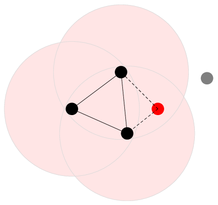
Then, we will repeat these two steps to obtain a growing network. Through studying the relationship between the total number of edges and the number of nodes in the network, , we can test the super-linear growth law.
Although the growing process is very simple and seems homogenous, the resulting network is very uneven both in time and space. First, the new agent is added in the system in a random place of the geometric space, but only if the random place is surrounded by existing agents, the new place will be occupied. Thus the density of existing agents is uneven in the geometric space, the network itself can be regarded as a result of “crystalization”. Second, the growing process is uneven in time because a much slower growing speed is expected in the initial process than the following steps.
However, in the simulation, we have to use a trick to avoid the problem of random searching on an infinite space: a new coming agent’s coordinate is not randomly assigned in the whole geometric space but a much smaller subset , where in the simulations, are minimum and maximum coordinates along all dimensions. In a word, the new coming agent is from a -dimensional box covering all existing agents randomly. This trick can accelerate our program dramatically but take no effect on the final results.
II.1 One Dimensional Model
Let’s consider the simplest case of our basic model, the geometric space is a one dimensional line, i.e., . In this simplest case, the super-linear growth phenomenon can be generated.

Figure 2 shows three simulations with different . We found at first all the simulations show super-linear growth, that is the number of edges v.s. the number of nodes in different time step has a power law relation with exponent larger than one. Second, all the curves of v.s. almost overlap each other on the plot which means the fittings by equation 1 have nearly same parameters. So, the exponents in equation 1 are independent on the parameter . This point can be confirmed by the larger scale simulations as shown in 3.

We observed clearly both and fluctuate around the mean values in different . Therefore, the super-linear growth phenomenon doesn’t dependent on the parameter .
II.2 Two Dimensional Model
Besides the basic phenomena shown in the 1-d model, 2-d model shows more interesting patterns. In this case, the geometric space itself can be illustrated by a 2-d picture. And the network formed by the model is a spatial network, so we can show the networks in different steps.

From figure 4, we know that the growing network in the geometric space is very uneven. We found the density of agents in the center of the geometric space is much higher than the peripheral places. Actually, the network in the 2-d geometric space is a fractal. That is the number of occupied lattice scales as the measurement size with the power law exponent (fractal dimension) . This point can be confirmed by the box-counting method, and the fractal dimensions is calculated in different time steps.

According to the box-counting method, we know the asymptotic fractal dimension is about . All the dimensions during the simulation are in between 1 and 2, therefore, the spatial networks are fractals.
II.3 Three Dimension Model
So far all the geometric spaces we have discussed are very abstract. In this subsection we will discuss a more concrete model: an interaction network of a city. Each node on the network is an individual living in the city, and the links between the nodes stand for the interactions (e.g. phone connection or friendship connection). The geometric space is a 3 dimensional Euclidean space in which two dimensions stand for the geographic space (since a city locate on a 2-dimensional plane of course) and the left single dimension is the similarity space. The basic matching rules are the same as the previous model settings. Hence, a connection is built only if two individuals locate very closed in the geographic space and have common interests (similarities).
In this model, all the phenomena we have discussed in last sections can be also observed. For example, the super-linear exponent is about , the fractal dimension of the network in 3-d space is about . While the projection of the network on the geographic space (2-d world) is also a fractal with dimension around being smaller than the one’s in the 2-d model. Thus the complexity of the 2-d projection of the 3-d network is smaller than the 2-d model because the new introducing dimension of the model make the matching criterion stricter.
Besides the fractal dimension of the network, we can also study the relationship between area and population which is comparable to the empirical studies in cities[20, 21]. In our model, we calculate city’s area by the following method. On the 2-d geographic space, we select a specific resolution as our observational scale. Then we use the given resolution to rasterize the whole geographic space, after that, we count the number of occupied boxes as the area just like the box-counting method in the fractal dimension calculation. Because the box occupied by multiple agents is treated as one unit of area, the increase speed of area is much slower than the speed of population increasing. Therefore, a sub-linear area-population relationship can be obtained as shown in figure 6

The area and population has a sub-linear power law relation:
| (3) |
Where, is the area of cities, and is the exponent. As shown in figure 6, all s are smaller than 1 and fall into the interval . This result is consistent with the observed exponents of real cities[20, 21]. We also show how the area-population relation depend on resolution. As the size of the box increases, increases also. Because city is a fractal object, the area as a macro measurement is dependent on the measurement scale certainly.

We can use the similar method to study the similarity space and found similar sub-linear law between diversity (different types of features) and population,
| (4) |
In figure 7, all the exponents s are around 0.3 which are much smaller than and more stable with respect to different resolutions.
Beyond the spatial properties and super-linear growth, we can also discuss other network features, and how do they change with the size of the system.


The degree distributions are not power laws but Weibull distributions. This is inconsistent with the empirical observation that the degree distributions are heavy tails. However, the clustering coefficient asymptotically unchange with the size of the network. This is also observed in empirical data[14].
Interestingly, through the simulations in 1,2 and 3 dimensions, we found the super-linear growth exponents depend not on but the spatial dimension (as shown in figure 10). To see how does super-linear growth exponent decay with the spatial dimension, we have done more experiments as shown in figure 11.


III Model Extensions
We have known what diverse and interesting patterns can the basic model exhibit, however, we can add a little of complexity on the basic one to make it closer to the reality. We will mainly consider several possible extensions. Firstly, we can study the geometric space with limitations. Secondly, we can add more heterogeneity in our model.
III.1 Finite Geometric Space
We will firstly extend our model to a finite geometric space. The simplest finite one that we can imagine is the unit interval on the real line. In this case, the super-linear exponent will depend on the interaction radius because the space is not scale-free anymore but have a maximum characteristic scale which is the upper bound of the radius. So, figure 12 shows different straight lines with different .

As we observed, the slope of the straight line, i.e. the super-linear exponent increases with the interaction radius . Even when the radius is large enough so that the scale is comparable with the maximum range of the geometric space itself, then the power law exponent is approaching the maximum possible value .
The unevenness of time, i.e., the waiting time between two agents adding in the network, can be investigated in this extended model. In section II, we have mentioned that a trick has to be used to accelerate the simulation process otherwise infinite time should be waited to add a new node when the geometric space is infinite. However, in this extension, we can directly simulate the whole random searching process without using this trick. In every time step, a new agent with a random position in the interval is added and survive with the condition that some old agents are close to him. Therefore, as time goes by, the growing speed of the whole network will be accelerated since the number of existing nodes become larger and larger. Instead plotting the waiting time between any two survival agents, we study the cumulative time, i.e. the total time elapse so far versus the total number of agents survived before . We found a asymptotic power law between these two variables.
| (5) |

From figure 13, we know the time intervals between two agents added into the whole network scales with the size of the network. And the exponent decreases with the interaction radius . When the radius is comparable with the scale of the geometric space, the exponent is approaching . Therefore, the growing process is actually a fractional dynamical process.
III.2 Finite Resolution
In the previous subsection, we have considered the upper bound of the size of the geometric space, the lower bound will be considered in this subsection.
At first, we can model the whole geometric space as a discrete cellular space. Each agent can only occupy one single cell. So the new node can only exist only if (1) they can build a link with at least one existing agent; (2) the new agent’s position in the geometric space is not occupied by any existing agent. By adding this new rule, we find the super-linear exponent is dependent on the interaction radius .
We set the minimum resolution as 1, and the maximum range of the geometric space as in all the following simulations. The interaction radius changes from to , the dependence of super-linear exponents on the radius in all space is shown in figure 14

We see in all cases when , the exponents are close to 1, which means the networks are very regular and like lattices. As the interaction radius increases, this constraint becomes weak, so the exponents will increase also. When is in the intermediate stage, the exponent s are always independent on because both the upper limitation and lower limitation have no any constraints on the systemic processes. The stationary exponents are almost identical to the ones in the free geometric cases. When is big enough, the upper bound of the geometric space will influence the behaviors of the s, so the exponents increase with the interaction radius to reach the maximum value . In these extensions, we know the parameter can affect the super-linear exponent due to the space limitation effect.
III.3 Heterogenous Models
We found the degree distributions of the basic model are not power laws as showed in many empirical networks. The essential reason is the homogeneity of the basic model, i.e. all the interaction radiuses are the same. This strong assumption is not supported by real life. Thus, in this subsection, we will consider a heterogenous model with random interaction radius.
In the first attempting, we suppose of each agent is a random number following exponential distribution, so the cumulative function of this variable is,
| (6) |
In this way, we can generate both super-linear growth and scale-free degree distribution patterns. That is the resulted degree distribution has a power law tail.
| (7) |
where, is the random variable for degrees, is the lower degree of power law tail, is its exponent. As increases, the heterogeneity of the degrees becomes larger. Figure 15 shows the cumulative degree distributions of several networks with different values.

Exponential distribution of is not the only choice, we can use other distribution density function to reproduce the power law degree distribution and super-linear growth pattern. For example, we replace the formula 6 to:
| (8) |
That means follows the half normal distribution (in each time step, draw a random number with normal distribution and take the absolute value). Figure 16 shows the degree distributions.

Comparing figure 15 and 16 we know the exponent of the degree distribution in normal distribution model is larger than the one in exponential distribution model. That means the heavy tail phenomenon is more insignificant than the former case.
To see how do the exponents and change with the parameters and , we have conducted larger scale experiments. The results are shown in figure 17. Both exponents and are almost invariant when and change. And because all the experiments are done in 2-d space, the exponent is almost identical to the values in the basic model. Therefore, although we have to introduce two new parameters and , the super-linear exponent is independent on them.

IV Discussion
In this paper, we introduce a new growing network model called growing random geometric graph. Actually, this is a modelling framework that can be used to model various complex networks and other systems. One of the main advantages of these models is they all exhibit super-linear growth or densification, accelerating growth phenomenon.
Besides the super-linear growth behavior, this simple model can also show a lot of scaling behaviors. We used a set of exponents to characterize these scalings. is the fractal dimension of the spatial network in the space, is the exponent of area and population, characterize the scaling between diversity of similarities and population, describe the power law relation between time and the size of the system and is the power law exponent of the degree distribution in the extended model. All these scaling behaviors indicate that the growing random geometric graph is an anomalous object that is governed by some unknown fractional dynamics. Further studies, especially the mathematical analysis are deserved.
Although we have discussed several interesting extensions toward the original model, more extensions are needed. For example, we can grow the network not only in the Euclidean space but other interesting space, e.g. hyperbolic space[22]. And other possible matching rules can be considered. Maybe more interesting phenomena will emerge.
Finally, this is only the first step of this model, both the theoretical analysis and empirical tests are needed in the future studies.
Acknowledgements.
Thanks for the discussions with Prof. Bettencourt in Santa Fe Institute, doctor Wu in Hong Kong city university and Prof. Wang and Chen in beijing normal university, acknowledges the support from the National Natural Science Foundation of China under Grant No. 61004107.References
- [1] L. M. Bettencourt, J. Lobo, D. Helbing, C. Kuhnert, and G. B. West, Proc. Natl. Acad. Sci. U. S. A., 104, 7301 (2007)
- [2] L. M. Bettencourt, Research Policy, 36, 107 (2007)
- [3] L. Bettencourt and G. West, Nature, 467, 912 (2010), ISSN 0028-0836
- [4] L. M. A. Bettencourt, J. Lobo, D. Strumsky, and G. B. West, PLoS ONE, 5, e13541 (2010)
- [5] L. Wu and J. Zhang, Physical Review E, 84, 026113 (2011)
- [6] D. C. v. Leijenhorst and T. P. v. d. Weide, Inf. Sci. Inf. Comput. Sci., 170, 263¨C272 (2005).
- [7] L. Lu, Z.-K. Zhang, and T. Zhou, 1002.3861 (2010), doi:10.1371/journal.pone.0014139.
- [8] J. Zhang and T. Yu, Physica A: Statistical Mechanics and its Applications, 389, 4887â?896 (2010), ISSN 0378-4371.
- [9] S. Arbesman, J. M. Kleinberg, and S. H. Strogatz, Physical Review E, 79, 016115 (2009).
- [10] S. N. Dorogovtsev and J. F. F. Mendes, arXiv:cond-mat/0204102 (2002).
- [11] S. N. Dorogovtsev and J. F. F. Mendes, arXiv:cond-mat/0106144 (2001), adv. Phys. 51, 1079 (2002).
- [12] J. Leskovec, J. Kleinberg, and C. Faloutsos, in Proceedings of the eleventh ACM SIGKDD international conference on Knowledge discovery in data mining, KDD ’05 (ACM, New York, NY, USA, 2005) pp. 177–187, ISBN 1-59593-135-X.
- [13] J. Leskovec, D. Chakrabarti, J. Kleinberg, C. Faloutsos, and Z. Ghahramani, J. Mach. Learn. Res., 11, 985 (2010), ISSN 1532-4435.
- [14] M. Schläpfer, L. M. A. Bettencourt, M. Raschke, R. Claxton, Z. Smoreda, G. B. West, and C. Ratti, arXiv:1210.5215 (2012).
- [15] L. Bettencourt, SFI working paper (2012).
- [16] R. J. Williams and N. Martinez, Nature, 404, 180 (2000).
- [17] M. Penrose, Random Geometric Graphs (Oxford University Press, 2003) ISBN 9780198506263.
- [18] M. E. J. Newman and R. M. Ziff, arXiv:cond-mat/0101295 (2001), doi:10.1103/PhysRevE.64.016706, phys. Rev. E 64, 016706 (2001).
- [19] A.-L. Barabási and R. Albert, Science, 286, 509 (1999), ISSN 0036-8075, 1095-9203.
- [20] S. Nordbeck, Geografiska Annaler. Series B, Human Geography, 53, 54 (1971), ISSN 04353684, ArticleType: primary_article / Full publication date: 1971 / Copyright © 1971 Swedish Society for Anthropology and Geography.
- [21] Y. Lee, Environment and Planning A, 21, 463 (1989).
- [22] F. Papadopoulos, M. Kitsak, M. n. Serrano, M. Boguñá, and D. Krioukov, Nature, 489, 537 (2012), ISSN 0028-0836.