Quantum heat fluctuations of single particle sources

Recent years have witnessed a surge of interest in on-demand sources for single particles in mesoscopic and nanoscale systems. This interest was motivated by the experimental progress [2, 1, 3, 4, 5, 6, 7] on fast, accurate single particle emitters, with operation frequencies reaching the GHz regime. Fast and accurate emitters are key elements in the efforts to obtain a quantum standard for the Ampere [8]. In addition to metrological applications, coherent on-demand sources, emitting regular streams of single particle wavepackets, are of great, fundamental importance. As recently demonstrated [5], sources implemented with edge states in the quantum Hall regime [1, 6] open up for quantum coherent few-electron experiments [9, 10, 11, 12, 13, 14] as well as put in prospect quantum information processing [15, 16, 17] with clocked single and entangled two-particle sources. Large efforts have also been put into characterising the properties of on-demand sources via the electrical current and its fluctuations [18, 20, 19, 21, 22, 23, 24, 25, 26].

Although the low-frequency charge emission of ideal on-demand sources is noiseless, the emitted heat fluctuates [27]. These fluctuations are ubiquitous for quantum coherent sources; particles emitted during a time shorter than the drive period ${\mathcal{T}}$ have an uncertainty in energy larger than $\hbar/{\mathcal{T}}$. Acting as emitters of quantum heat fluctuations, coherent on-demand sources comprise ideal components for tests of heat fluctuation relations [28, 29, 30, 31] in the quantum regime [32] or for investigating the statistics of temperature [33, 34] or heat transfer [35] fluctuations in mesoscopic systems. In addition, the large versatility of system parameters and pulse protocols [5, 6] for on-demand sources allows for a tailoring of the spectral properties of the emitted wavepackets.

In this work we provide a compelling illustration of the fluctuation properties of system consisting of a generic coherent on-demand source coupled to a hot-electron probe, see Fig. 1. It is shown that the temperature and potential fluctuations induced at the probe, besides fundamental constants, depend only on the source frequency and the spectral properties of the emitted wavepackets. For a wide range of parameters, the quantum fluctuations are found to dominate over the classical ones. In addition, the full distribution of the fluctuations reveals a direct proportionality between the cumulants of the marginal temperature and potential distributions, allowing for an experimental investigation of the temperature fluctuation via correlators of the potential fluctuations.

We first discuss the energy emission properties of an isolated, optimal on-demand source, emitting a train of single particle wavepackets $|\Psi\rangle$, equally spaced ${\mathcal{T}}=2\pi/\omega$ in time, see Fig. 1. The wavepackets, emitted on top of a filled Fermi sea, are superpositions of states at different energies,

where $\hat{b}^{\dagger}(\epsilon)$ creates a particle at energy $\epsilon>0$, $|0\rangle$ denotes the filled Fermi sea and $c(\epsilon)$ an amplitude normalised as $\int d\epsilon p(\epsilon)=1$, with $p(\epsilon)=|c(\epsilon)|^{2}$.

Although energy emission for individual electrons can be accessed via charge counting in weakly tunnel coupled systems [29, 31, 35], for on-demand sources operating in the GHz regime single-shot energy detection is presently not possible. Instead one has to consider schemes where the effect of collecting a large number $N\gg 1$ of emitted electrons, with a fluctuating total energy $E$, become measurable. For an on-demand source characterized by $p(\epsilon)$, the statistical distribution $P(E)$ of the total energy can conveniently be written

where $NF(\xi)$ is the cumulant generating function for $P(E)$ and $N=t_{0}/{\mathcal{T}}$ is the number of particles with $t_{0}\gg{\mathcal{T}}$ the measurement time. The different cumulants of $P(E)$ are obtained by successive derivatives of $F(\xi)$ with respect to $\xi$, giving for the average and the width

where $\langle..\rangle=\int d\epsilon..p(\epsilon)$. Importantly, the direct relation between the statistics of $E$ and $p(\epsilon)$ of the individual wavepackets depends crucially on the ideal operation of the source. Irregular wavepacket emission or scattering in space or energy between emission and detection will make $P(E)$ dependent on other factors. We stress that on-demand sources which emit subsequent, identical electron and hole wavepackets [1], (and hence no net charge) have the same heat emission properties as pure electron sources with twice the drive frequency $\omega$.

To access the heat fluctuation properties of the source we consider an on-demand source coupled to a probe in the hot-electron regime, an electrically and thermally floating terminal, see Fig. 1. The source-probe setup is implemented in a conductor in the quantum Hall regime, allowing to minimise scattering, elastically or inelastically, between particle emission and collection in the probe. Particles emitted from the source propagate to the probe along the lower edge state. From the probe, emitted particles follow the upper edge and are collected in a grounded electronic reservoir kept at low (here zero) temperature.

In the hot-electron probe, injected particles thermalize rapidly, via electron-electron interactions, on the time scale $\tau_{e-e}$. This time is much shorter than the typical time $\tau_{d}$ a particle spends inside the probe before being reemitted. However, the energy exchange with the lattice phonons takes place on the time scale $\tau_{e-ph}$, much longer than $\tau_{d}$. The electron distribution in the probe is then in a quasi-equilibrium state, characterized by a chemical potential and temperature. In order to prevent charge and energy pile-up in the floating probe, both the chemical potential $\mu_{p}(t)$ and temperature $T_{p}(t)$ develop fluctuations in time. The potential fluctuations can be detected by present day electrical measurements. Importantly, as we now show, the potential fluctuations also provide direct information on the quantum heat fluctuation of the source, via $p(\epsilon)$ of the individual particles.

To present a clear and compelling picture we analyse the temperature and potential fluctuations within a Boltzmann-Langevin approach. We write $T_{p}(t)=\bar{T}_{p}+\delta T_{p}(t)$ and $\mu_{p}(t)=\bar{\mu}_{p}+\delta\mu_{p}(t)$ with $\bar{T}_{p},\bar{\mu}_{p}$ average quantities and $\delta T_{p}(t),\delta\mu_{p}(t)$ fluctuating Langevin terms. The statistics of $\delta T_{p}(t)$ and $\delta\mu_{p}(t)$ is determined from underlying quantum properties, as discussed below. First we consider the average quantities $\bar{T}_{p}$ and $\bar{\mu}_{p}$. The starting point is the operator for charge current at the probe [36], $\hat{I}_{p}^{c}(t)=\int d\epsilon d\epsilon^{\prime}e^{i(\epsilon-\epsilon^{\prime})t/\hbar}\hat{i}_{p}(\epsilon,\epsilon^{\prime})$ where $\hat{i}_{p}(\epsilon,\epsilon^{\prime})=(e/h)[\hat{b}^{\dagger}(\epsilon)\hat{b}(\epsilon^{\prime})-\hat{a}^{\dagger}(\epsilon)\hat{a}(\epsilon^{\prime})]$ with $\hat{b}^{\dagger}(\epsilon)[\hat{a}^{\dagger}(\epsilon)]$ creating particles incident on [emitted from] the probe. By analogy we write the operator for the heat current $\hat{I}_{p}^{h}(t)=\int d\epsilon d\epsilon^{\prime}e^{i(\epsilon-\epsilon^{\prime})t/\hbar}[(\epsilon+\epsilon^{\prime})/2-\mu_{0}]\hat{i}_{p}(\epsilon,\epsilon^{\prime})$, where $\mu_{0}=0$ is the chemical potential of the reservoir. Taking the quantum average with respect to the emitted source state, Eq. (1), and the state of the probe, and averaging over a time much longer than the period $\mathcal{T}$, we arrive at the dc component of charge and heat currents

where $g_{0}=e^{2}/h$ is the (single spin) conductance quantum and $l_{0}=(\pi k_{B}/e)^{2}/3$ the Lorentz number. To account for both types of sources discussed, we introduced $\sigma=0$ for sources emitting no net charge and $\sigma=1$ for sources emitting one electron per cycle. We note that the first and the second terms of $\langle I_{p}^{c}\rangle$ and $\langle I_{p}^{h}\rangle$ in Eq. (4) are the currents emitted by the source and the probe respectively. The conditions for zero average charge and heat currents at the probe, $\langle I_{p}^{c}\rangle=0$ and $\langle I_{p}^{h}\rangle=0$, give from Eq. (4)

Importantly, $\bar{\mu}_{p}$ and $\bar{T}_{p}$ depend only on the source properties $\omega$ and $\langle\epsilon\rangle$ and fundamental constants [5]. We note that $\langle\epsilon\rangle>\hbar\omega/2$ follows along the lines of Ref. [37].

Turning to the temperature and chemical potential fluctuations [38], the quantities of primary experimental interest are the low frequency correlators $\langle(\delta\mu_{p})^{2}\rangle\equiv(1/t_{0})\int dtdt^{\prime}\langle\delta\mu_{p}(t)\delta\mu_{p}(t^{\prime})\rangle$ and equivalently for $\langle(\delta T_{p})^{2}\rangle$, with the measurement time $t_{0}\gg\mathcal{T}$. We first point out that the total fluctuations of charge and heat currents $\Delta I_{p}^{c}$ and $\Delta I_{p}^{h}$ are made up by bare fluctuations $\delta I_{p}^{c}$ and $\delta I_{p}^{h}$ and fluctuations due to the varying temperature and voltage of the probe, $\partial_{T_{p}}\langle I_{p}^{x}\rangle\delta T_{p}$ and $\partial_{\mu_{p}}\langle I_{p}^{x}\rangle\delta\mu_{p}$, with $x=c,h$, as

suppressing for shortness the time dependence of the fluctuations. From Eqs. (4) and (6), taking into account the conservation of charge and heat current fluctuations, i.e. $\Delta I_{p}^{c}=0$ and $\Delta I_{p}^{h}=0$, we can express $\delta\mu_{p}$ and $\delta T_{p}$ in terms of the bare charge and heat fluctuations as

The correlators $\langle(\delta\mu_{p})^{2}\rangle$ and $\langle(\delta T_{p})^{2}\rangle$ can be thus expressed in terms of low frequency correlators of bare charge and heat fluctuations $\langle\delta I_{p}^{x}\delta I_{p}^{y}\rangle\equiv(1/t_{0})\int dtdt^{\prime}\langle\delta I_{p}^{x}(t)\delta I_{p}^{y}(t^{\prime})\rangle$. The correlator of the Langevin terms $\langle\delta I_{p}^{x}(t)\delta I_{p}^{y}(t^{\prime})\rangle$ is evaluated by taking the quantum average of the corresponding correlator of current operators $\hat{I}_{p}^{c}$, $\hat{I}_{p}^{h}$ following Ref. [36]. We arrive at

The potential fluctuations $\langle(\delta\mu_{p})^{2}\rangle$ are proportional to the average temperature, typical for equilibrium systems [38]. In contrast, the temperature fluctuations $\langle(\delta T_{p})^{2}\rangle$ are a sum of two physically distinct terms. The first term, the classical fluctuations, is proportional to $\bar{T}_{p}$ and results from the finite temperature of the probe and would be present even if the injected particles had a well defined energy, i.e. $\Delta\epsilon=0$. The second term, quantum fluctuations, is proportional to $(\Delta\epsilon)^{2}$ and is a direct result of the uncertainty of the energy of the injected particle. Importantly, for a broad range of drive frequencies $\omega$ and wavepacket mean energies $\langle\epsilon\rangle$ and widths $\Delta\epsilon$, the quantum term dominates over the classical one. We also point out that there are no correlation between the voltage and the temperature fluctuations, i.e. $\langle\delta\mu_{p}\delta T_{p}\rangle=0$.

In order to investigate the presence of quantum heat fluctuations in higher order potential correlations, and also to provide a complete picture of the temperature and potential fluctuations, we turn to the full probability distribution. To relate to the average and fluctuation correlators above, we introduce a dimensionless potential $\mu=(1/h)\int_{0}^{t_{0}}dt\mu_{p}(t)$, and temperature $T=(1/h)\int_{0}^{t_{0}}dtk_{b}T_{p}(t)$, fluctuating quantities integrated over the measurement time $t_{0}$. The joint probability distribution $\mathcal{P}_{t_{0}}(\mu,T)$ can be conveniently written in terms of a cumulant generating function $G(\chi,\theta)$ as

with $\chi$ and $\theta$ counting fields for $\mu$ and $T$ respectively. From $G(\chi,\theta)$ the low frequency cumulants are then, by construction, obtained from successive derivatives with respect to the counting fields, giving $t_{0}\langle\delta T_{p}^{n}\delta\mu_{p}^{m}\rangle=(-ih)^{n+m}k_{b}^{-n}\partial^{n}_{\theta}\partial^{m}_{\chi}G(\chi,\theta)|_{\chi,\theta=0}$.

To determine $G(\chi,\theta)$ we first spell out the relations between the time scales in the problem. The potential $\mu_{p}(t)$ fluctuates on the time scale given by the RC-time, $\tau_{RC}$, while the temperature $T_{p}(t)$ typically fluctuates on the time scale of the dwell-time in the probe, $\tau_{d}$. We assume that the system is in the limit $\tau_{e-e}\ll\tau_{RC},\tau_{d}\ll\tau_{e-ph}$. Moreover, we consider periods of the source, $\mathcal{T}$, and measurements time such that $t_{0}\gg\tau_{d},\tau_{RC}\gg\mathcal{T}$. On time scales $\tau$ such that $\mathcal{T}\ll\tau\ll\tau_{d},\tau_{RC}$ the statistics of net transferred energy $E_{p}$ and charge $Q_{p}$ in the probe can be described by the source generating function $\tau h_{s}(\lambda,\xi)$ with

with $F(\xi)$ given in Eq. (2) and the probe generating function $\tau h_{p}(\lambda,\xi,E_{p},Q_{p})$ with [39, 40, 41]

where $f_{p}(\epsilon)=f_{p}(\epsilon,\mu_{p},T_{p})$ and $f(\epsilon)$ are the probe and the reservoir distribution functions (see Fig. 1) and $\xi$ and $\lambda$ are the counting fields for $E_{p}$ and $Q_{p}$ respectively. The energy $E_{p}$ and charge $Q_{p}$ are related to $T_{p}$ and $\mu_{p}$ as $E_{p}=\nu[\mu_{p}^{2}/2+(\pi k_{b}T_{p})^{2}/6]$ and $Q_{p}=\nu e\mu_{p}$, where $\nu$ is the density of states in the probe. Working within the framework of the stochastic path integral formalism [42, 41], we can then express $G(\chi,\theta)$ as a path integral over all configurations of $E_{p}$ and charge $Q_{p}$ during the measurement. In the long time limit we have

where $S(Q_{p},E_{p},\lambda,\xi)=t_{0}[i\theta k_{b}T_{p}/h+i\chi\mu_{p}/h+h_{p}(Q_{p},E_{p},\lambda,\xi)+h_{s}(\lambda,\xi)]$. Similar to Refs. [40, 41, 33], the integral in Eq. (12) is solved in the saddle point approximation. Inserting the solutions for $Q_{p},E_{p},\lambda,\xi$ into $S(Q_{p},E_{p},\lambda,\xi)$ we arrive at

recalling that $N=t_{0}/\mathcal{T}$, where $F(z)\equiv F(\xi)|_{i\xi=z/\hbar\omega}$ and $z$ is found from the relation $z^{2}[dF/dz+\sigma/2]=-(\pi^{2}/6)(1-\sqrt{1-2g})^{2}$ with $g(\chi,\theta)=(3/\pi^{2})[(i\chi)^{2}/2+i\theta]$. From Eq. (13) we note several important things. First, by expanding $G(\chi,\theta)$ in terms of $\chi$ and $\theta$ we see that the first two cumulants reproduce the results in Eqs. (5) and (8). Second, all the even chemical potential cumulants, from the first two terms in Eq. (13), can be expressed in terms of the temperature cumulants as

a consequence [43] of the counting fields entering via $g(\chi,\theta)$.

The full distribution $\mathcal{P}_{t_{0}}(\mu,T)$ can be found (to exponential accuracy) by solving the integral in Eq. (9) in the saddle point approximation. We obtain the compact expression

where $\bar{\mu}=t_{0}\bar{\mu}_{p}/h=\sigma N$ and the saddle point solution $\theta^{*}$ is found from the relation $dF/dz|_{z=z^{*}}+\sigma/2=-(\pi^{2}/6)(Tq^{*}/N)^{2}$, with $z^{*}=N(q^{*}-1)/(q^{*}T)$ and $q^{*}=\sqrt{1-i6\theta^{*}/\pi^{2}}$. Importantly, Eq. (15) shows that the potential $\mu$ displays Gaussian fluctuations, of width $\sqrt{T}$, around the average $\bar{\mu}$ for any given temperature $T$. Hence, the marginal potential distribution $\mathcal{P}_{t_{0}}(\mu)=\int dT\mathcal{P}_{t_{0}}(\mu,T)$ is symmetric around $\bar{\mu}$, albeit not Gaussian. Moreover, the marginal distribution for the temperature $\mathcal{P}_{t_{0}}(T)=\int d\mu\mathcal{P}_{t_{0}}(\mu,T)$ is given by $\ln\mathcal{P}_{t_{0}}(T)=-iT\theta^{*}+G(0,\theta^{*})$.

To illustrate our results we evaluate $\ln\mathcal{P}_{t_{0}}(T)$ for two distinct cases. First, as a reference, we consider the generic Gaussian spectral distribution $p(\epsilon)=1/(\sqrt{2\pi}\Delta\epsilon)e^{-(\epsilon-\langle\epsilon\rangle)^{2}/(2(\Delta\epsilon)^{2})}$. Taking the classical limit, with $\Delta\epsilon\ll\langle\epsilon\rangle$, we get the simple result

with $\bar{T}=t_{0}k_{b}\bar{T}_{p}/h$ the average value of $T$. The log probability is plotted in Fig. 2. For small fluctuations $T-\bar{T}\ll\bar{T}$ the distribution is Gaussian while for $T\ll\bar{T}$ the probability is suppressed $\mathcal{P}_{t_{0}}(T)\propto e^{-\pi^{2}\bar{T}^{2}/(6T)}$, guaranteeing $\mathcal{P}_{t_{0}}(T)\rightarrow 0$ for $T\rightarrow 0$. The probability for large fluctuations $T\gg\bar{T}$ is suppressed as $\mathcal{P}_{t_{0}}(T)\propto e^{-T\pi^{2}/6}$. For finite but small width $\Delta\epsilon\ll\langle\epsilon\rangle$, the log probability in Eq. (16) is multiplied by the term $1+(\Delta\epsilon/\langle\epsilon\rangle)^{2}\bar{T}^{2}\pi^{2}/(12TN)$ for $T\sim\bar{T}$, a small quantum correction.

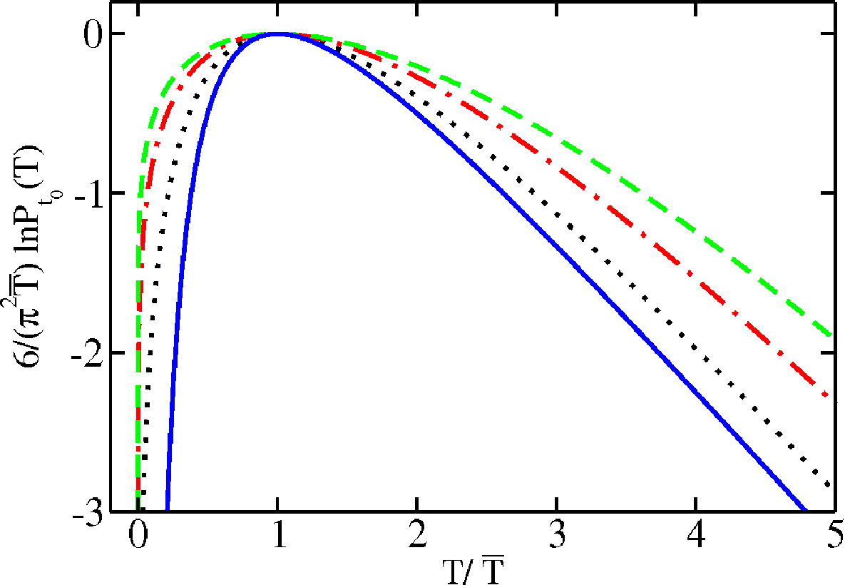
In contrast, for an exponential distribution $p(\epsilon)=(1/\langle\epsilon\rangle)e^{-\epsilon/\langle\epsilon\rangle}$ derived in Ref. [19] for adiabatic particle emission and investigated in Ref. [18], we find the probability

where $q^{*}=(\alpha/2+\sqrt{\alpha\bar{T}/T+1+\alpha^{2}/4})/(T/\bar{T}+\alpha)$ and $\alpha=\pi\sqrt{\langle\epsilon\rangle/(6\hbar\omega)}$. The probability distribution is plotted in Fig. 2 for different values of $\alpha$. We see that for increasing $\alpha$, corresponding to slower drive $\omega$ and/or larger average wavepacket energies $\langle\epsilon\rangle$, the distribution gets increasingly broad and deviates strongly from the classical one in Eq. (16).

In conclusion we have investigated the quantum fluctuations of the heat current emitted from a single particle source. We show that these quantum heat fluctuations can be detected via electrical potential fluctuations of a probe coupled to the source. For typical parameters [1] $2\pi\omega\sim 1GHz$ and $\langle\epsilon\rangle\sim 0.1meV$ we get $\bar{\mu}_{p}\sim 5\mu eV$ and $\bar{T}_{p}=0.2K$, demonstrating the experimental feasibility of our proposal.

We acknowledge valuable discussions with C. Flindt and M. Büttiker. We acknowledge support from the Swedish VR.

References

- [1] G. Fève, A. Mahé, J.-M. Berroir, T. Kontos, B. Plaçais, D. C. Glattli, A. Cavanna, B. Etienne, and Y. Jin, Science 316, 1169 (2007).
- [2] M. D. Blumenthal, B. Kaestner, L. Li, S. Giblin, T. J. B. M. Janssen, M. Pepper, D. Anderson, G. Jones, and D. A. Ritchie, Nature Phys. 3, 343 (2007).
- [3] A. Fujiwara, K. Nishiguchi, and Y. Ono, Appl. Phys. Lett. 92, 042102 (2008).
- [4] J.P. Pekola, J. J. Vartiainen, M. Möttönen, O.-P. Saira, M. Meschke, and D. V. Averin, Nature Phys. 4, 120 (2008).
- [5] E. Bocquillon, F. D. Parmentier, C. Grenier, J.-M. Berroir, P. Degiovanni, D. C. Glattli, B. Plaçais, A. Cavanna, Y. Jin, and G. Fève, Phys. Rev. Lett. 108, 196803 (2012).
- [6] F. Hohls, A. C. Welker, Ch. Leicht, L. Fricke, B. Kaestner, P. Mirovsky, A. Müller, K. Pierz, U. Siegner, and H. W. Schumacher, Phys. Rev. Lett. 109, 056802 (2012).
- [7] S. Giblin, M. Kataoka, J. D. Fletcher, P. See, T. J. B. M. Janssen, J. P. Griffiths, G. A. C. Jones, I. Farrer, and D. A. Ritchie, Nat. Commun. 3, 930 (2012).
- [8] J.P. Pekola, O.-P. Saira, V. F. Maisi, A. Kemppinen, M. Möttönen, Y. A. Pashkin, and D. V. Averin, arxiv:1208.4030v1.
- [9] S. Ol’khovskaya, J. Splettstoesser, M. Moskalets, and M. Büttiker, Phys. Rev. Lett. 101, 166802 (2008).
- [10] J. Splettstoesser, S. Ol’khovskaya, M. Moskalets, and M. Büttiker, Phys. Rev. B 78, 205110 (2008).
- [11] C. Grenier, R. Hervé, E. Bocquillon, F. D. Parmentier, B. Plaçais, J.-M. Berroir, G. Fève, and P. Degiovanni, New J. Phys. 13, 093007 (2011).
- [12] S. Juergens, J. Splettstoesser, and M. Moskalets, Europhys. Lett. 96, 37011 (2011).
- [13] G. Haack, M. Moskalets, J. Splettstoesser, and M. Büttiker, Phys. Rev. B 84, 081303 (2011).
- [14] G. Haack, M. Moskalets, and M. Büttiker, arXiv:1212.0088.
- [15] J. Splettstoesser, M. Moskalets, and M. Büttiker, Phys. Rev. Lett. 103, 076804 (2009).
- [16] L. Chirolli, V. Giovannetti, R. Fazio, and V. Scarani, Phys. Rev. B 84, 195307 (2011).
- [17] Y. Sherkunov, N. d’Ambrumenil, P. Samuelsson, and M. Büttiker, Phys. Rev. B 85, 081108 (2012).
- [18] M. Moskalets, P. Samuelsson, and M. Büttiker, Phys. Rev. Lett. 100, 086601 (2008).
- [19] J. Keeling, A.V. Shytov, and L. S. Levitov, Phys. Rev. Lett. 101, 196404 (2008).
- [20] B. Kaestner, V. Kashcheyevs, S. Amakawa, M.D. Blumenthal, L. Li, T.J.B.M Janssen, G. Hein, K. Pierz, T. Weimann, U. Siegner, and H. W. Schumacher, Phys. Rev. B. 77, 153301 (2008).
- [21] N. Maire, F. Hohls, B. Kaestner, K. Pierz, H. W. Schumacher, and R. J. Haug, App. Phys. Lett. 92, 082112 (2009).
- [22] A. Mahé, F. D. Parmentier, E. Bocquillon, J.-M. Berroir, D. C. Glattli, T. Kontos, B. Plaçais, G. Féve, A. Cavanna, Y. Jin, Phys. Rev. B. 82, 201309(R) (2010).
- [23] M. Albert, C. Flindt, and M. Büttiker, Phys. Rev. Lett. 107, 086805 (2011).
- [24] F. Battista and P. Samuelsson, Phys. Rev. B 83, 125324 (2011); Phys. Rev. B 85, 075428 (2012).
- [25] F. D. Parmentier, E. Bocquillon, J.-M. Berroir, D.C. Glattli, B. Plaçais, G. Fève, M. Albert, C. Flindt, and M. Büttiker, Phys. Rev. B 85, 165438 (2012).
- [26] T. Jonckheere, T. Stoll, J. Rech, and T. Martin, Phys. Rev. B 85, 045321 (2012).
- [27] M. Moskalets and M. Büttiker, Phys. Rev. B 80, 081302(R) (2009).
- [28] A. Altland, A. De Martino, R. Egger and B. Narozhny, Phys. Rev. B 82, 115323 (2010).
- [29] D.V. Averin, and J. Pekola, Phys. Rev. Lett. 104, 2206601 (2010); Europhys. Lett. 96, 67004 (2011).
- [30] B. Küng, C. Rössler, M. Beck, M. Marthaler, D.S. Golubev, Y. Utsumi, T. Ihn, and K. Ensslin, Phys. Rev. X. 2, 011001 (2012).
- [31] O.-P. Saira, Y. Yoon, T. Tanttu, M. Möttönen, D. V. Averin, and J. P. Pekola, Phys. Rev. Lett. 109, 180601 (2012).
- [32] M. Esposito, U. Harbola, and S. Mukamel, Rev. Mod. Phys. 81, 1665 (2009).
- [33] T.T. Heikkilä and Y. V. Nazarov, Phys. Rev. Lett. 102, 130605 (2009).
- [34] M.A. Laakso, T.T. Heikkilä and Y. V. Nazarov, Phys. Rev. Lett. 104, 196805 (2010).
- [35] R. Sánchez and M. Büttiker, Europhys. Lett 100, 47008 (2012).
- [36] M. Büttiker, Phys. Rev. B 46, 12485 (1992).
- [37] J. E. Avron, A. Elgart, G. M. Graf, and L. Sadun, Phys. Rev. Lett. 87, 236601 (2001).
- [38] Ya. Blanter and M. Büttiker, Phys. Rep. 336, 1 (2000).
- [39] L. S. Levitov and G. B. Lesovik, JETP Lett. 58, 230 (1993).
- [40] M. Kindermann and S. Pilgram, Phys. Rev. B 69, 155334 (2004).
- [41] S. Pilgram, Phys. Rev. B 69, 115315 (2004).
- [42] S. Pilgram, A.N. Jordan, E. V. Sukhorukov, and M. Büttiker, Phys. Rev. Lett. 90, 206801 (2003).
- [43] The factorial growth of the cumulants with order is in agreement with general predictions in C. Flindt et al. Proc. Natl. Acad. Sci. USA 106, 10116 (2009).