Anomalous Higgs Couplings as a Window to New Physics
Abstract
The initial data on the production and decay of the Higgs boson reported significant deviations from the Standard Model (SM) expectations, prompting much speculation about its couplings to the other particles. Although the latest data has veered towards conformity with the SM, there is yet room for a sizable deviation from the SM values of the coupling of the Higgs boson with , and to a smaller extent, of that with and . Keeping the fluid nature of the data in mind, this opens up an interesting avenue to explore regarding unitarity of gauge boson scattering and the stability of the electroweak vacuum in the presence of anomalous couplings. We show that, for some typical benchmark points, unitarity in gauge boson scattering breaks down between 1 and 10 TeV. We also show that if there are no new light degrees of freedom, the Higgs quartic coupling becomes negative at around the same point, making the electroweak vacuum unstable. Thus, some new ultraviolet completing new physics is demanded at that scale to cancel both these anomalous behaviours if such deviations from the SM couplings are indeed established.
pacs
14.80.Bn, 11.80.EtI Introduction
The recent discovery of a resonance by both the ATLAS [1] and the CMS [2] collaborations at the Large Hadron Collider (LHC) has led to intense activity. This has been accentuated by the fact that initially both the groups reported excesses—over the Standard Model (SM) backgrounds—in multiple channels and concentrated at nearly the same (125–126 GeV) reconstructed mass. Supported by evidence from the Tevatron [3], this has naturally led to euphoria in the community. However, even though the resonance is obviously a boson, its identification with the long-awaited Higgs particle of the standard electroweak theory is not yet certain.
While the observed diphoton decay mode excludes the possibility of the said resonance being a spin-1 particle, other non-trivial assignments are, as yet, possible. This is notwithstanding the analysis in Ref. [4] where the pure scalar hypothesis is found to be favoured over the pure pseudoscalar hypothesis for the said resonance. Furthermore, even if the said assignment is proven, that still does not uniquely identify the observed particle to be the SM Higgs boson, there is still enough room for new physics (NP) resulting in modified Higgs couplings with the SM particles. For one, the diphoton (the channel permitting the cleanest measurement of the mass) rate was significantly above the expectations even in late 2012, and is not yet in full conformity with the SM. While these are yet early days to claim a discrepancy, the observed patterns have led to intense speculations about the nature of this particle and the ramifications of this discovery for a host of scenarios of physics beyond the Standard Model (BSM) [5, 6, 7]. At this juncture, it must be recognised that the purported discrepancies, if any, could just be a manifestation of the inherent uncertainties in QCD calculations, both in the perturbative and the non-perturbative regimes [8]. On the other hand, ratios of signal rates (such as that between the diphoton and the four-lepton final states) are relatively free of such uncertainties and constitute a more robust signature of a deviation from the SM expectations [9]. A framework for this has been discussed in Ref. [10], where the scale factors , parametrizing the deviation of Higgs decay width or production cross section, were defined; the production cross section for or the decay width for has an extra multiplicative scale factor when compared with the SM predictions.
In view of the state of affairs (compounded by the fact that no other distinct departure from the SM has been observed at the LHC), the authors of Ref. [7] effected an interesting phenomenological study. Considering all of the Higgs couplings, whether tree-level or loop-induced, to be unrelated and free parameters, as well as allowing for an invisible decay mode for the Higgs, they used the observations (both low-energy, such as precision electroweak observables, as well as the recent data) to obtain a best fit to the same. In as much as no underlying physics assumptions (other than Lorentz invariance) were made for this sector (i.e., no patterns were imposed on the anomalous couplings of the Higgs, whether to the gauge bosons or to the fermions), this constitutes, perhaps, the most general investigation to the possible nature of physics just beyond the SM scale.
One might parametrize the Higgs effective coupling to and gauge bosons to be
| (1) |
where is the vacuum expectation value (VEV) of the Higgs. Within the SM, and all equal unity. Allowing these couplings (as also others, which are not germane to the discussions here) to vary independently, Ref. [7] finds that the “best fits”, according to data available in early July 2012, are given by
| (2) |
The fits F1 and F2 were performed holding to be real. Similarly, F2 and F3 demanded custodial symmetry. The constraint on custodial symmetry breaking, given by the oblique parameter , is so strong that it is natural to impose . Note that for these points, all the other parameters were held at their best fit values respectively and not at the SM values.
One must, however, be aware of the fact that the rapid influx of data makes the best fit points vulnerable to change even over a very short period of time, and analyses based on the latest data present in Moriond 2013 are now available in the literature [11, 12, 13]. For example, Ref. [11] obtained and , assuming the custodial symmetry and using all Higgs production and decay data along with electroweak precision observables; whereas not imposing this symmetry leads to [12] and . Note that while our benchmark points F1–F3 may no longer remain the best fit values, they are still within the 95% allowed range. One should also bear in mind that the internal disagreements between the various data sets cannot yet be wished away and the accumulation of further data can swing the pendulum either way. Furthermore, the deviations allowed for by even the Moriond data are quite significant. In particular, the top quark Yukawa coupling still has a very large uncertainty and can potentially be negative. In fact, such a negative coupling, and consequently a constructive interference between the top-mediated and the -mediated triangle diagrams (in place of a destructive interference as in the SM), was touted to be a plausible way out from the apparent excess in in July 2012 data. The effects of such anomalous top Yukawa coupling already received attention much before the discovery of the Higgs boson, e.g., in the context of baryogenesis [14] or unitarity violation in gauge boson scattering [15]. The latter will be particularly relevant for our subsequent discussion.
As the exact nature of the “best fit” would again change once more data is included in the fit, we do not consider the cases of Eq. (2), or even the later values, to be sacrosanct, but treat them only as indicative of such fits. It is worth noting that once custodial symmetry is imposed, the deviations from the SM, viz. are much smaller than (this also holds, albeit weakly, for F1). Although still larger than what naive dimensional analysis would suggest (for a new physics scale GeV), such could, presumably, be the result of quantum corrections (possibly, though, in a theory that is either strongly coupled or has a non-trivial ultraviolet completion). The large change of is, however, a more complicated story and constitutes the bulk of this paper.
One notes that such a change is also indicated in ATLAS and CMS analyses [16, 17] based on their data and the formalism developed in Ref. [10]. Taking and (so that the custodial symmetry is respected), the ATLAS Collaboration found, within 68% confidence limit,
| (3) |
The CMS Collaboration, on the other hand, found the best fit at . However, each of the two collaborations analysed only their own data set, and also did not consider the possibility that the Higgs could decay into any new particles. Thus, the fit in [7] encompasses a wider amount of data. With this caveat, it is easy to appreciate the relatively minor differences in the fits.
While the process of pinning down the various couplings of the Higgs continues as data pour in, it is also necessary to subject our observations to theoretical consistency checks. For example, one important role of the Higgs boson is to ensure partial wave unitarity in various scattering processes. The role of longitudinal scattering, for example, in unveiling possible new physics in anomalous gauge self-interaction, even in the absence of any well-defined resonance, has been discussed in Ref. [18]. If the couplings of the Higgs turn out to have non-standard values, then the fine balance required for unitarity is destroyed, and one has to set a cut-off scale for the theory [19]. In this work, we derive values of this cut-off scale for various levels of departure of the Higgs-fermion-antifermion interactions from their standard values. Side by side, we also examine the implications of such modified interaction strengths on the issue of vacuum stability (essentially arising from the radiatively corrected quartic coupling potentially turning negative). And, based on the above considerations, we make some remarks on how the existence of additional particles can restore balance to the whole scenario, if indeed the recently observed scalar has anomalous coupling strengths.
The rest of the paper is arranged as follows. In Section II, we discuss some theoretical issues pertaining to the choice of these best-fit points; in particular, we would like to spend some time on the point F3, which includes a nontrivial phase in the top Yukawa coupling. In Section III, we discuss the unitarity of and scattering with such benchmark points. The evolution of the scalar quartic coupling is discussed in Section IV. While we do not go into details about models that can produce such effective couplings, some relevant remarks are made in Section V. We summarize and conclude in the Section VI. Some calculational details as well as a compendium of necessary formulae are put in the appendices.
II Some Theoretical Issues
Let us first make a few comments on the point F3, where a complex top Yukawa coupling is indicated. This immediately raises very pertinent and interesting questions as to the possible sources of such an anomalous coupling. While mixing effects (whether in the Higgs sector or in the fermion sector) can and do cause significant deviations in the coupling, the magnitude of the deviation is never so large unless the new states are both very light and have complicated quantum number assignments. Similarly, such a large anomalous coupling is not expected from loop-corrections (owing to some as-yet-unobserved states) unless the said sector couples very strongly to the observed one11 1 This observation applies equally to fit F1 as well as to of F2.. In particular, the existence of a non-zero in Eq. (1) ostensibly renders the Hamiltonian to be non-Hermitian. Although this, at the first glance, would seem to lead to non-unitary time evolution, it has been shown that field theories based on a non-unitary Lagrangian [20] could accommodate a unitary -matrix. This, however, requires a redefinition of the metric in the Hilbert space, and with such a modified metric, the -matrix is unitary if all stable particles have a positive-definite norm. Such a redefinition, however, requires that propagators and Feynman diagrams (indeed, the entire perturbation theory) be redefined adequately [21]. This introduces a whole new panoply of problems, such as those dealing with electroweak precision measurements as well as classic tests of quantum electrodynamics such as the Lamb shift or anomalous magnetic moment of the electron (and, its cousin, the muon). This seems to be too big a price to pay and we shall, hence, turn our attention to simpler alternatives.
As is well-known, such an absorptive part can arise from loop-corrections within a Hermitian theory if there exists an intermediate state that can be on-shell. However, the existence of such a state begs many questions. For one, such particles would necessarily be light and should have manifested themselves not only in Higgs decays, but also in other collider processes. This is particularly so, for, by definition, such a state would be part of an doublet, which, in turn, would immediately call for similar contributions to the absorptive parts of other effective vertices (with or without the Higgs). Not only this, such a light state should have been produced directly too. In particular, the antecedents would have required that they be produced at a clean environment such as LEP-II (as also the Tevatron). No signs of either such production, or the inducing of absorptive parts in other couplings have yet been observed. Similarly, one cannot ascribe this phase due to say, an exchange of an unknown (set of) particle in the “-channel” of a loop with the on-shell particles being some light SM state such as the . Although a phase can appear in such a case, it actually encapsulates the final state rescattering of the said light particles (i.e. , with rescattering, in howsoever complicated a fashion, to the final state of interest, viz. ), and has little to do with an effective vertex.
Furthermore, the very act of calculating loops with such an ansatz for the origin of the phase (as attempted in the literature) is fraught with danger. An effective theory can be obtained (starting from an ultraviolet completion) only on integrating out fields more massive than the scale at which the effective theory is being utilized. By its very definition, then, the light fields that ostensibly led to the phase cannot be integrated out and must be included in all loop corrections, whether for the Higgs production and/or decay, or for processes involving other particles, such as the . Such inclusion will, naturally, lead not only to significant changes in such observables, but, most often, tend to cancel the effect of the phase (seeing that it is absent in the complete theory and was but an artefact of a perturbative calculation).
It should also be realized that, for , the top quark lines at this vertex cannot be on the positive energy mass-shell. Thus, the application of Cutkowsky rules is not straightforward; nor is the identification of with the discontinuity across a cut arising from a physical region singularity. In other words, the existence of a non-zero in Eq. (1) cannot be motivated from any simple physics. Indeed, such non-Hermiticity is a subtle issue in quantum field theory [21], and even if such a phase were to occur due to some hidden sector exchanges, we cannot include it in an effective Lagrangian (which is a must for any loop calculations) in any straightforward manner. We shall, henceforth, consider the top Yukawa coupling to be real, albeit admitting the possibility of an anomalous component to it. Thus, our benchmark point F3 will be parametrized by . Note that this does not invalidate Ref. [7], for when they hold , they still find that the best fit requires with the deviation from the SM being substantial22 2 Indeed, we find the admission of a non-zero to be rather unwarranted, given that the -distribution is very flat for (see Fig. 4 of Ref. [7])..
It is interesting to note that a nonzero phase had been introduced earlier in the top Yukawa coupling, albeit in a different context [14]. Wishing to incorporate CP violation in this interaction (motivated by a desire to address baryogenesis), the authors of Ref. [14] augmented the SM Lagrangian by an effective operator of the form
| (4) |
where denotes a (real) effective coupling owing its origin to higher-dimension terms. In the unitary gauge, this yields
| (5) |
over and above the SM term. Clearly, a non-zero leads to CP violation. This coupling, though, is markedly different from the ansatz of Ref. [7], as it emanates from an Hermitian effective Lagrangian unlike in the other case. Furthermore, the pseudoscalar term (which, essentially, is the only one to see a non-zero value of the phase ) in the coupling above contributes only incoherently to and is, thus, of little consequence (at least within the effective theory paradigm).
An anomalous top Yukawa coupling (even if real) brings in its own complications. Within the SM, all couplings are dictated by gauge invariance33 3 For example, the Yukawa couplings are uniquely given in terms of the masses.. While deviations are indeed possible once one enlarges the ambit of the theory, gauge invariance would require that these either be associated with higher-dimensional effective operators, or be the consequence of mixings between states (were new states to be admitted). Each of these eventualities would imply correlated deviations in other couplings, and, on occasions, the introduction of new ones. Any uncorrelated deviation, such as that of Eq. (1) can only be the result of an additional term in the Lagrangian of the form
| (6) |
where, for simplicity, we have chosen . Such a term, of course, explicitly breaks . While its inclusion may seem to militate against the gauge dogma, note that Eq. (6) could just represent the relevant part of the BSM physics, with other terms being hidden for unknown reasons. Thus, the breaking of gauge invariance might be an artefact of restricting ourselves to be close to the augmented SM, which acts only as a low-energy effective theory, while gauge invariance is again restored when we go to the full theory at a high energy. In the effective theory, due to the apparent loss of gauge invariance, the mass and the Yukawa coupling of the fermions, in particular the top quark, get decoupled, and this apparent loss has other profound implications. As is well known, unitarity in gauge boson scattering (in particular, the longitudinal modes) is inextricably linked to gauge invariance. While any loss of unitarity due to could, in principle, be restored on inclusion of other terms in , the scale at which such a loss is seen (if one considers alone) would point to the scale of the new theory that underlies such a deviation. Similarly, the existence of would have non-trivial consequences for the renormalization group evolution of the couplings in the theory as well for considerations such as the stability of the vacuum.
III Unitarity Bounds
III.1 Unitarity and
In a phenomenological study of the Higgs boson, while all its couplings could be varied independently [7], it makes sense to concentrate on the dominant ones. Within the SM, these are the ones with the top quark and the weak gauge bosons. Maintaining the Lorentz structures to be identical to those within the SM, these can be parametrized as in Eq. (1), but categorically with .
Clearly the effective Lagrangian in Eq. (1) would have non-trivial effects on a host of scattering processes, notably on where . As is well-known, partial wave unitarity for such scattering processes depends crucially on the couplings being those mandated by invariance alongwith renormalizability. Thus, could, in principle destroy the same for, say, . This particular scattering proceeds through a set of seven Feynman diagrams, namely a four-point contact interaction, two -channel diagrams mediated by the and the (or, in the unbroken symmetry phase, by the ), two analogous -channel ones and, finally, one each of – and –channel Higgs-mediated diagrams. With the trilinear (quartic) gauge boson vertices scaling as () where is a typical momentum transfer, and the polarization vector for the longitudinal vector boson going (for large ) as , it is obvious that each of the individual pure-gauge diagram contributions to the amplitude goes as . The gauge theory antecedents of the vector-boson self-couplings ensure that the leading terms cancel identically leaving behind a behaviour. Once the Higgs-mediated diagrams are included, even the contributions cancel, and on integrating the remaining terms over the phase space, one obtains a cross section in consonance with the Froissart bound44 4 Although the presence of a massless photon in the -channel results in a collinear singularity, this does not violate the Froissart bound. Indeed, this singularity disappears (as it should) when higher order corrections are taken into account.. Clearly, this cancellation is contingent upon the Higgs couplings being just so, and allowing for would result in additional contributions from the Higgs-mediated diagram to the amplitude resulting in a bad high-energy behaviour.


In Fig. 1, we show the consequent behaviour of the cross sections for a few representative values of . Note that even for small values of that are allowed at present, the cross section grows anomalously and hence it is easy to ascertain that such a theory loses unitarity at a few TeVs at best55 5 It is instructive to note that the loss of unitarity occurs not only for (corresponding to best fit with custodial symmetry [11]), but also for (best fit without custodial symmetry [12]). and a new theory needs to be around, and, by implication, within the reach of the LHC.
It might be argued, though, that such a deviation in could well be accompanied by others in the gauge boson self couplings, evoking memories of a non-linearly realized symmetry, or at the very least, higher-dimensional terms in an electroweak chiral Lagrangian. While it seems plausible that such correlated deviations could preserve unitarity, it can be seen that simultaneous restoration in all possible channels is difficult to achieve within the ambit of phenomenologically acceptable deviations [22]. However, even if this were to be possible, constraints appear from another sector that we now turn to. This is of particular importance as the deviations in the fits F2 and F3 are relatively small and could shrink further once more data is taken into account.
III.2 Unitarity and
As already mentioned, of the SM particles, the Higgs couples with an unsuppressed strength only to the weak gauge bosons and the top. We have already discussed the consequences of deviations to the former and, now, concentrate on the latter. In analogy to the discussion in the preceding section, this coupling plays a crucial role in processes such as , to which the following diagrams contribute:

As can be ascertained from arguments mirroring those in the preceding section, the amplitude that grows most strongly with energy pertains to annihilation to . Indeed, the Higgs diagram contribution goes as for . If the coupling deviates from the SM value, the cancellation of the leading term with the non-Higgs diagrams would be imperfect and the amplitude would grow with energy, thereby violating the Froissart bound at some scale. While it may be argued that it is only the combination that comes into play, note that the needed for the fits can neither compensate for the required nor is such a large deviation consistent with scattering. Similarly, large deviations in the vertex can be ruled out from the measurements of single-top production at the Tevatron [23] and the LHC [24], as well as from B physics observables such as the mass difference of neutral B meson eigenstates.
This study is best done in terms of the partial wave amplitudes defined as
where is the Lorentz invariant amplitude, is the scattering angle and the Legendre functions. Unitarity demands that
and it is the amplitude that gives the strongest bound. In particular, the most sensitive probe is given by the amplitude for the particular helicity combination
with the case for being identical. Denoting the velocities of the particles in the center-of-mass frame by and , one obtains66 6 The details of the calculations are given in Appendix A.
| (7) | |||||
where and . We have assumed here that the gauge couplings of the top quark are unaltered77 7 Note that a significant variation from is strongly disfavoured by constraints from flavour physics. from those in the SM. While no direct measurement of the vertex is available, once one considers the vertex to be in consonance with the SM (also indicated to be so by a host of observables such as single top production, top decays as well as -meson phenomenology), custodial symmetry mandates that the coupling should also be as postulated within the SM. The collinear singularity that appears in the large- limit—attested to by the logarithmic term—is identical to that within the SM and disappears once higher order corrections are taken into account. Any violation of unitarity is, then, proportional to the deviation of the product from unity.

In a similar vein, we can consider , to which the diagrams of Fig. 3 contribute. Once again, proves to be the most sensitive probe. Denoting the coupling of the left–(right–) handed top states with the by (), this is given by
| (8) | |||||
where .
In Fig. 4, we show the variation of the aforementioned with the center-of-mass energy. As expected, a deviation of the couplings from the SM values cause a significant change in the magnitude of . Indeed, for the most favourable cases of Ref. [7] unitarity would be violated at TeV, while for the more recent fits [11, 12], this would occur at TeV. In other words, this indicates the maximal energy scale of the effective theory, beyond which a new theory must be operative.


It might be argued, though, that much of the unitarity violation exhibited in Fig. 4 may be caused by the shifts in and . As discussed in the preceding section, such deviations are strongly disfavoured by considerations involving gauge boson scattering. Indeed, it can be explicitly checked that the violation of unitarity owes itself to a negative value for the product (engendered by a negative ). Furthermore, the particular values chosen for the anomalous couplings were dictated by the ‘best fits’ corresponding to a set of data that might soon be overwhelmed by new data. In view of this, it is worthwhile to examine the consequences of having a nonzero alone, while maintaining all other couplings to their SM values. Indeed, as an examination of Eqs. (7) and (8) suggests, the extent of unitarity violation is determined solely by .
In Fig. 5 we display this data in terms of iso- contours in the – plane. Only the white part of the figures bounded by the curves are in consonance with unitarity, and the shaded regions are ruled out. Once again, this shows that even if all the other couplings were left unmolested, a large deviation in alone would run afoul of unitarity constraints well within a few TeVs. This certainly holds not only for the most favoured values quoted by Ref. [7] but also for a very large fraction of their C.L. allowed regions.


IV Vacuum Stability
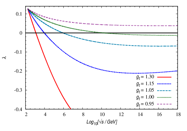
If the consideration of unitarity persuades us to set some cut-off scale to the SM augmented by the anomalous couplings, it is important to check whether the theory respects all other constraints, experimental as well as theoretical. A case in point is the issue of vacuum stability, which demands that the Higgs quartic coupling has to be positive. Once we allow the possibility of a deviation from the SM Yukawa coupling, namely , the RG evolution for the Higgs quartic coupling would be affected too. The RG equation for involves only even powers of top Yukawa coupling , which, with , is just times the SM top Yukawa coupling. Thus the sign of is irrelevant, with the evolution depending only on its magnitude.
We use the two-loop -function for , following Refs. [25]. For completeness, they are also quoted in Appendix B. We use the two-loop matching conditions, as given in Ref. [26], to match the data, viz.
| (9) |
to their corresponding values at .
We show the evolution of the scalar quartic coupling , and the top Yukawa coupling, in Fig. 6. This shows that the electroweak vacuum might get unstable if is even slightly greater than unity, and the point where the instability sets in depends rather sensitively on . For example, the vacuum becomes unstable at an energy as low as about GeV for . At the one-loop level, the negative term proportional to , coming from a top-mediated box diagram, is responsible for this. Thus, both F2 and F3 would indicate the presence of new physics GeV on this account (the unitarity bounds are stronger, though), while F1 seems to be safe. While these shifts parallel those engendered by the errors on the top quark mass measurement itself, there are subtle differences. For one, the shift in that the fittings favour are much larger than the experimental errors in (– according to various estimates). Moreover, the deployment of the matching conditions in the two cases would differ.
At the same time, we must be cautious about taking these numbers too literally. The calculations hold only if the new physics responsible for the change in the top Yukawa coupling is either above the scale where instability sets in (so that those new degrees of freedom are still frozen), or the effective interaction involves only SM fields but with a new operator structure. In particular, the apparent consistency of F1 cannot be depended on, once the physics responsible for unitarity violation is turned on.

V Contemplating Possible Avenues
While we have delineated the problems that beset an effective theory wherein the coupling of the recently glimpsed Higgs-like resonance to the top quark, the and the are reset from the SM values to those obtained from phenomenological best fits, we have not indicated any source for the same. For example, the generation of a large (but real) anomalous coupling to be the result of either large quantum corrections or mixings with as yet undetected states. The latter possibility would, of course, require such states to be relatively low-lying, and in fact not too separated from the corresponding known SM states. Were it indeed to be so, all arguments about unitarity or triviality would necessarily need to be revised. Since an exhaustive treatment is not possible owing to the paucity of independent data, as well as the enormity of the task, we examine some simple alternatives. Viewed differently, while the arguments in the previous sections point to the necessity of having a relatively low cutoff, we now consider some possible realizations of the same.
Before we delve into the specifics, let us consider some generic issues.
- •
It might be argued that a negative would necessitate the existence of a second source of electroweak symmetry breaking and that this would imply relatively light new states. However, a close examination of the same shows that while the first part of the argument does hold, the second depends on implicit assumptions about the new sector. For example, one could well admit a second higgs doublet or a strongly interacting sector (such as topcolor), perhaps coupling only to the top quark. At the cost of some fine tuning (or introduction of additional symmetries, analogous but not identical to those in Little Higgs models), one could easily raise the mass scale for the new particles to a few TeVs. What the preceding arguments do show, however, that, independent of the fine tuning, this scale has to be lower than TeV.
- •
The introduction of any such ultraviolet completion would have an impact on the running of the Higgs quartic couplings. This is irrespective of whether this new sector couples to the SM Higgs at the tree level. This would, presumably, cure the potential problem with vacuum stability. However, unless the entire theory is known, an accurate computation of this effect is not possible, and we will not attempt to do so.
V.1 Gauge boson scattering
To begin with, let us consider the effect of . While unequal values for and do violate custodial symmetry, the most visible consequences appear in electroweak precision observables and can be neutralized by arranging for compensating custodial breaking in other sectors of the theory. Indeed, this has been included in the fitting of Ref. [7]. As for the unitarity violation in gauge boson scattering, curing it would require the introduction of additional contributions to the amplitude. The simplest possibility88 8 As explained earlier, we do not consider modification of the gauge boson self couplings. would be to postulate the existence of another scalar, say , whose couplings parallel those of in Eq. (1), but with the corresponding couplings being , viz.
| (10) |
Assuming that this new scalar has a mass , the restoration of unitarity for would require that
| (11) |
with the three constraints emanating from considerations of , and (and crossed processes) respectively. While the requirements might seem trivial at first sight, note that these are actually three conditions on two variables. Moreover, the “best fit points” and, indeed, most of the good fit part of the parameter space found in [7] requires , thereby necessitating negative . While this roadblock could be circumvented by postulating a wrong sign for the scalar kinetic term, such a solution brings along its own problems. Note, though, that this would still not guarantee the existence of a simultaneous solution to all three of the above constraints. However, the extent of unitarity violation could be minimized so as to push the scale of violation significantly higher.
The situation simplifies considerably if the scalar is not an ad hoc degree of freedom, but part of another Higgs multiplet that contributes to electroweak symmetry breaking. While only certain representations would guarantee at the tree-level, it is possible, in principle, to arrange multiple vacuum expectation values for a multitude of representations and carefully tune them to maintain this relation [27, 28]. Obtaining effective for at least one such scalar (to be identified with the observed resonance) requires that at least one of these representations must be higher than a doublet [28]. Typically, though, would not be maintained. It should be realized that, now, it is not just one new scalar that we would have, but an entire multiplet. This, of course, would change eqs.(11) to include additional terms, thereby making it easier to satisfy all three conditions. (This is despite the fact that gauge symmetry would relate several of the new couplings.) The behaviour of the potentially offending cross sections (equivalently, the partial wave amplitudes) would change too; interim phases of growth with would be seen, especially as a new Higgs threshold is approached. For very large though, the Froissart bound would be seen to be validated.
Yet another way to obtain is to postulate a new scalar with non-standard kinetic terms for at least one of the two (the new scalar and ) such that significant kinetic mixing occurs. An example of this is afforded by the radion in warped models [28].
From scalars, we turn our attention to vector bosons as restorers. Unitarizing gauge boson scattering in Higgs-less models through the introduction of new vector bosons has been investigated in Refs. [29, 30]. Clearly, the couplings must satisfy certain conditions. In the presence of a Higgs (albeit with altered couplings), the relations of Ref. [29, 30] have to be altered suitably. The required changes are straightforward, at least as far as the scattering of the SM gauge bosons is concerned. It must be noted, though, that the introduction of such vector bosons introduces the possibility of a pair of them emanating from, say, annihilation. The latter scattering would be associated with its own unitarity violation problems, and, just as in the case of the Higgs-less models, one would have to introduce a tower of such gauge bosons. The tower, in principle, is an infinite one and can be truncated only at the cost of admitting unitarity violation at some scale (or, equivalently, appealing to some ultraviolet completion). Similarly, all the trilinear (and quartic) couplings between this set of vector bosons must satisfy sum rules, the character of which will depend on whether they couple to .
Finally, it should be noted that this role of unitarity restoration is not restricted to only scalars and vector bosons, but can also be assumed by higher-spin bosons. The inclusion of the latter, though, brings a whole new set of problems to the table, and we desist from any discussion of the same.
V.2 Gauge boson annihilation to fermion pairs
The introduction of a new scalar could, in principle, restore unitarity for such processes. Once again, denoting the coupling of to a pair through a form analogous to Eq. (1), but with , we can express the conditions for unitarity restoration as
| (12) |
As before, we are faced with the problem of simultaneous solution of both these constraints, especially once are determined from considerations of gauge boson scattering (see preceding section). Of course, with the amplitude here growing only as , a lack of cancellation can be accommodated to a relatively larger degree, yet postponing unitarity violation to TeV, or even later.
The main problem, though, is that the best fit requires . This, of course, entails having , or, in other words, rather large couplings for the . Of particular importance is the fact that the inclusion of scalars in larger representations of (and ascribing vacuum expectation values to them) as in the preceding section, not only does not help, but actually worsens the situation. The reason is easy to see. As such large representations would not couple to the top quark (barring non-renormalizable terms), if the wavefunction of the observed resonance were to carry a significant fraction of such a state, its coupling to the top would actually be reduced from the SM value. This, of course, goes against current observations. Thus, one is left with the problem of arranging a large . Within the ambit of a phenomenological Lagrangian, this is admissible and can be arranged by invoking a suitably large Yukawa coupling (renormalizable if the extra higgs field is a doublet, and nonrenormalizable otherwise). However, note, that such a Yukawa coupling would grow rapidly with energy and one would be faced with a Landau pole. An alternative could be to consider new fermions or gauge bosons which may not couple to our familiar Higgs doublet. However, it is easy to see that this does not help as long as the latter behave canonically.
To summarise, the introduction of a new (set of) scalars with carefully constructed couplings seems to offer the simplest solution to the conundrum. A strictly phenomenological approach, on the other hand, would be given by ascribing form factor behaviour to the deviations. For example, consider the replacement
This, clearly would restore unitarity at large energies. This has the further advantage that this permits an examination of the behaviour of the coupling at different energies, thereby permitting some insight into the structure of the deviation once more data is available. Of course, a more generic form factor can be used instead, even correcting for the lack of gauge invariance that the simple-minded expression above entails. This, though, takes us to the regime of electroweak chiral Lagrangians and we shall not delve into it any further.
VI Future Outlook and Conclusions
Assuming that the Higgs couplings to the SM fields are arbitrary but consistent with general principles like Lorentz invariance and hermiticity, we tried to see whether the present data gives any hint of new physics beyond the SM. A particularly sensitive probe is offered by considerations of unitarity in gauge boson scattering. We have considered several such scattering amplitudes, for polarized as well as unpolarized gauge bosons, and partial wave unitarity is seen to break down at about TeV for coupling values preferred by the fits.
Even if this can be prevented by restoring the and vertices to their SM values (especially since the best fits, anyway, call for only small deviations), we are still faced two rather interesting issues. Indeed, the most important parameter in the study is the top quark Yukawa coupling, which might even have a sign opposite to that of the SM prediction. because of the apparent excess of Higgs to diphoton decay rate. We explored the consequences of such a wrong-sign coupling.
There are two places where the wrong-sign Yukawa coupling can play havoc. The first is the unitarity in gauge boson annihilation to a pair. This effect can be traced to a term in the scattering amplitude which is proportional to the product of the top quark Yukawa coupling and the coupling. With the sign flip of this term, the amplitudes grow up instead of going down and one sees unitarity violation at TeV. Thus, this indicates some new physics which takes over at a few TeV scale and restores unitarity as well as gauge invariance, which is apparently broken by Eq. (6).
The second place is the stability of the electroweak vacuum. The Higgs quartic coupling becomes negative if the magnitude of the top Yukawa coupling increases even a little from its SM value (only is important here, and not the sign of ). The point where the vacuum becomes unstable is a sensitive function of , but for our benchmark points, occur between 1 and 10 TeV, a region already indicated by the unitarity violation. Again, this asks for some new degrees of freedom, which couple to the Higgs and make the vacuum stable (so these should better be bosonic in nature). Of course, whether the cutoff of the theory is at the Planck scale or at a few TeVs does not affect the rate as this must always be finite.
It might be argued that the departures from standard couplings as suggested by the data are based on global analyses, where other couplings are simultaneously assuming non-standard values. This could be construed to mean that a complete analysis will have to take into account the role of the other modified couplings in the evolution of as well as in ensuring unitarity in scattering phenomena. While, as a principle, this is certainly true, note that our analysis has included all of the relevant dimension-4 terms that can be written down in terms of the SM fields alone. Although the inclusion of subdominant terms would alter the quantitative details of our conclusions, no qualitative change would be brought about.
Thus, if the initial trend—in particular the excess in diphoton channel—persists in the new data, this might lead to some indirect evidence of new physics which is lurking close. It is worthwhile to consider the possibility that the accumulation of further luminosity would reduce the discrepancy between the data and the SM expectations, without completely obliterating it. Were this to be the case, one would still need small but non-zero values for one or more anomalous couplings. A direct measurement of such small changes in the effective couplings would be well-nigh impossible, especially in the LHC environment. Pending future experiments, considerations of unitarity and vacuum instability would then consist of the best “evidence” for a relatively low-lying threshold. However, if the effective couplings shift by less than 10% of their SM values, the minimum required scale for new physics would rise to TeV.
Recently, both ATLAS and CMS have updated their results for Higgs search at TeV. These include not only those for the channels that form the core of our analysis, namely [31, 32], [33, 34] and [35, 36], but also for others such as [37, 38]. Based on these, it has been variously claimed that the observations are almost perfectly in consonance with the SM expectations. However, a careful examination betrays a persisting lack of consistency between the various measurements. The large variations in the data, alongwith the data in [39, 40] as well as [41, 42] has led to subsequent fits [11, 12]. Although these are in the spirit of earlier fits [5, 6, 7], the incorporation of new data has led to a shift in the best fit values for the couplings somewhat away from those of Ref. [7]. Notwithstanding these changes, the most important message is that the values for can yet be far away from those within the SM. In particular, can be substantially different from unity [11, 12] (with the central issue of this paper still remaining a concern). It should be appreciated, though, that these are yet early days of Higgs physics and the central values may yet shift!
Note added.
While the work was being completed, we became aware of a similar work in progress [43].
Acknowledgements.
The authors thank Biswarup Mukhopadhyaya for collaboration during the early phase of the investigation and G. Rajasekaran for an insightful comment. D.C. thanks Debashis Ghoshal for useful discussions. R.I. was supported by CSIR, Government of India, under grant 09/045(0872)/2009-EMR-I. A.K. was supported by CSIR, Government of India (project no. 03(1135)/9/EMR-II), and also by the DRS programme of the UGC, Government of India.Appendix A Momenta, Polarizations and Helicity Amplitudes
In our calculations we have denoted the momenta of the particles as follows
| (13) |
where is the CM energy, and . in the appropriate cases.
The polarization vectors have been denoted as
| (14) |
where corresponds to the longitudinal and are the transverse polarizations. are as follows
| (15) |
The helicity states of top quarks are given by
| (16) |
From (16) we can get the 4-component Dirac spinors as
| (17) |
Here we have defined .
Using the momenta from (13), polarizations and helicity states from (14), (16) respectively and the taking the effective Lagrangian of Eq. (1), we get the helicity amplitudes for as
| (18) |
Similarly we get the helicity amplitudes for as
| (19) |
where . , and , the Weinberg angle.
Appendix B Beta Functions
We give the beta functions used in our calculation from the appendix of Ref. [44]. The beta function for a generic coupling is given as:
| (20) |
The beta functions are given, above but below any new degrees of freedom, by [25]:
| (21) |
In the above, is the quartic Higgs coupling, , the top Yukawa coupling, and are the and couplings respectively. As the evolution of involves itself rather than the SM top Yukawa coupling , no new RGE appears; the existence of a nontrivial manifests itself only through the replacement in each of the eqs.(21). Also note that our description is purely phenomenological and no dynamic origin is ascribed to (doing so would need a specific ultraviolet completion).
References
- [1]
G. Aad et al. [ATLAS Collaboration],
Phys. Lett. B 716, 1 (2012)
[arXiv:1207.7214 [hep-ex]];
G. Aad et al. [ATLAS Collaboration], Phys. Rev. D 86, 032003 (2012) [arXiv:1207.0319 [hep-ex]]. - [2] S. Chatrchyan et al. [CMS Collaboration], Phys. Lett. B 716, 30 (2012) [arXiv:1207.7235 [hep-ex]].
- [3] T. Aaltonen et al. [CDF and D0 Collaborations], Phys. Rev. Lett. 109, 071804 (2012) [arXiv:1207.6436 [hep-ex]].
- [4] S. Chatrchyan et al. [CMS Collaboration], Phys. Rev. Lett. 110, 081803 (2013).
- [5]
F. Bonnet, M. B. Gavela, T. Ota and W. Winter,
Phys. Rev. D 85, 035016 (2012)
[arXiv:1105.5140 [hep-ph]];
A. Azatov, R. Contino and J. Galloway, JHEP 1204, 127 (2012);
J.R. Espinosa, C. Grojean, M. Muhlleitner and M. Trott, arXiv:1202.3697 [hep-ph];
P.P. Giardino, K. Kannike, M. Raidal and A. Strumia, arXiv:1203.4254 [hep-ph];
T. Li, X. Wan, Y. Wang and S. Zhu, arXiv:1203.5083 [hep-ph];
M. Rauch, arXiv:1203.6826 [hep-ph];
M. Farina, C. Grojean, E. Salvioni, arXiv:1205.0011 [hep-ph];
J.R. Espinosa, M. Muhlleitner, C. Grojean and M. Trott, arXiv:1205.6790 [hep-ph];
J. Ellis and T. You, JHEP 1206 (2012) 140;
D. Carmi, A. Falkowski, E. Kuflik and T. Volanski, arXiv:1202.3144 [hep-ph];
M. Duhrssen, S. Heinemeyer, H. Logan, D. Rainwater, G. Weiglein and D. Zeppenfeld, Phys. Rev. D 70 113009 (2004);
R. Lafaye, T. Plehn, M. Rauch, D. Zerwas and M. Duhrssen, JHEP 0908 009 (2009);
M. Klute, R. Lafaye, T. Plehn, M. Rauch and D. Zerwas, arXiv:1205.2699 [hep-ph];
A. Azatov, R. Contino, D. Del Re, J. Galloway, M. Grassi and S. Rahatlou, arXiv:1204.4817 [hep-ph];
S. Dawson and E. Furlan, Phys. Rev. D 86, 015021 (2012) [arXiv:1205.4733 [hep-ph]];
F. Bonnet, T. Ota, M. Rauch and W. Winter, Phys. Rev. D 86, 093014 (2012) [arXiv:1207.4599 [hep-ph]]. - [6]
I. Low, J. Lykken and G. Shaughnessy,
arXiv:1207.1093 [hep-ph];
T. Corbett, O.J.P. Eboli, J. Gonzalez-Fraile and M.C. Gonzalez-Garcia, arXiv:1207.1344 [hep-ph];
P.P. Giardino, K. Kannike, M. Raidal and A. Strumia, arXiv:1207.1347 [hep-ph];
J. Ellis and T. You, arXiv:1207.1693 [hep-ph];
J.R. Espinosa, C. Grojean, M. Muhlleitner and M. Trott, arXiv:1207.1717 [hep-ph];
M. Montull and F. Riva, arXiv:1207.1716 [hep-ph];
D. Carmi, A. Falkowski, E. Kuflik, T. Volansky and J. Zupan, arXiv:1207.1718 [hep-ph];
S. Dawson, E. Furlan and I. Lewis, arXiv:1210.6663 [hep-ph]. - [7] S. Banerjee, S. Mukhopadhyay and B. Mukhopadhyaya, JHEP 1210, 062 (2012) [arXiv:1207.3588 [hep-ph]].
- [8] J. Baglio, A. Djouadi and R.M. Godbole, arXiv:1207.1451 [hep-ph].
- [9] S.S. AbdusSalam and D. Choudhury, arXiv:1210.3331 [hep-ph].
- [10] LHC Higgs Cross Section Working Group, A. David, A. Denner, M. Duehrssen, M. Grazzini, C. Grojean, G. Passarino and M. Schumacher et al., arXiv:1209.0040 [hep-ph].
- [11] A. Falkowski, F. Riva and A. Urbano, arXiv:1303.1812 [hep-ph].
- [12] P.P. Giardino, K. Kannikec, I. Masina, M. Raidal and A. Strumia, arXiv:1303.3570 [hep-ph].
- [13] J. Ellis and T. You, arXiv:1303.3879 [hep-ph].
- [14] X. Zhang, S.K. Lee, K. Whisnant and B.L. Young, Phys. Rev. D 50, 7042 (1994) [hep-ph/9407259].
- [15] K. Whisnant, B.L. Young and X. Zhang, Phys. Rev. D 52, 3115 (1995) [hep-ph/9410369].
- [16] ATLAS Collaboration note ATLAS-CONF-2012-127.
- [17] CMS Collaboration note CMS PAS HIG-12-045.
- [18] D. Espriu and B. Yencho, Phys. Rev. D 87, 055017 (2013) [arXiv:1212.4158 [hep-ph]].
- [19]
K. Cheung, C. -W. Chiang and T. -C. Yuan,
Phys. Rev. D 78, 051701 (2008)
[arXiv:0803.2661 [hep-ph]];
B. Bellazzini, C. Csaki, J. Hubisz, J. Serra and J. Terning, JHEP 1211, 003 (2012) [arXiv:1205.4032 [hep-ph]]. - [20]
T. D. Lee and G. C. Wick,
Nucl. Phys. B 9, 209 (1969);
T. D. Lee and G. C. Wick, Phys. Rev. D 2, 1033 (1970). - [21]
T.D. Lee, in Quanta, Chicago Univ Press, 260 (1970);
R. E. Cutkosky, P. V. Landshoff, D. I. Olive and J. C. Polkinghorne, Nucl. Phys. B 12, 281 (1969). S. Coleman, Acausality, in Erice 1969, Academic Press, NY, 282 (1970);
N. Nakanishi, Phys. Rev. D 3, 811 (1971);
T.D. Lee and G.C. Wick, Phys. Rev. D 3, 1046 (1971);
D. G. Boulware and D. J. Gross, Nucl. Phys. B 233, 1 (1984). - [22] M. Dahiya, S. Dutta and R. Islam, to appear.
- [23] Y. Peters [CDF and D0 Collaborations], arXiv:1210.7188 [hep-ex].
- [24]
ATLAS Collaboration,
ATLAS-CONF-2012-132;
CMS Collaboration, CMS-PAS-TOP-12-011. - [25]
M.B. Einhorn and D.R.T. Jones,
Phys. Rev. D 46, 5206 (1992);
M.-x. Luo and Y. Xiao, Phys. Rev. Lett. 90, 011601 (2003) [hep-ph/0207271];
M.E. Machacek and M. T. Vaughn, Nucl. Phys. B 222, 83 (1983);
M.E. Machacek and M. T. Vaughn, Nucl. Phys. B 236, 221 (1984);
M.E. Machacek and M.T. Vaughn, Nucl. Phys. B 249, 70 (1985). - [26] F. Bezrukov, M.Y. Kalmykov, B.A. Kniehl and M. Shaposhnikov, JHEP 1210, 140 (2012) [arXiv:1205.2893 [hep-ph]].
- [27] J.F. Gunion, H.E. Haber, G.L. Kane and S. Dawson, Front. Phys. 80, 1 (2000).
- [28] D. Choudhury, A. Datta and K. Huitu, Nucl. Phys. B 673, 385 (2003) [hep-ph/0302141].
- [29] C. Csaki, C. Grojean, H. Murayama, L. Pilo and J. Terning, Phys. Rev. D 69, 055006 (2004) [hep-ph/0305237].
- [30] Y. Nomura, JHEP 0311, 050 (2003) [hep-ph/0309189].
- [31] ATLAS Collaboration, ATLAS-CONF-2013-012; ATLAS-CONF-2012-091.
- [32] CMS Collaboration, CMS-HIG-13-001.
- [33] ATLAS Collaboration, ATLAS-CONF-2013-034.
- [34] CMS Collaboration, CMS-HIG-13-002.
- [35] ATLAS Collaboration, ATLAS-CONF-2013-030.
- [36] CMS Collaboration, CMS-HIG-13-005.
- [37] ATLAS Collaboration, ATLAS-CONF-2013-009.
- [38] CMS Collaboration, CMS-HIG-13-006.
- [39] ATLAS Collaboration, ATLAS-CONF-2012-170.
- [40] CMS Collaboration, CMS PAS HIG-12-044.
- [41] ATLAS Collaboration, ATLAS-CONF-2012-160.
- [42] CMS Collaboration, CMS-HIG-13-004.
- [43] G. Bhattacharyya, D. Das and P. B. Pal, Phys. Rev. D 87, 011702 (2013) [arXiv:1212.4651 [hep-ph]].
- [44] M. Holthausen, K.S. Lim and M. Lindner, JHEP 1202, 037 (2012) [arXiv:1112.2415 [hep-ph]].