跳到论文正文
W Papers独立论文阅读器 arXiv:1212.4529 论文正文 计算阅读时间 · 0%
引用这篇论文根据当前论文元数据生成,正式投稿前建议核对。


License: arXiv.org perpetual non-exclusive license
arXiv:1212.4529v2 [math.GT] 16 Nov 2014

The decategorification of bordered Heegaard Floer homology

Ina Petkova Address: Department of Mathematics, Rice University
Houston, TX 77005
Email address: ina@rice.edu
Abstract.

Bordered Heegaard Floer homology is an invariant for 33-manifolds, which associates to a surface FF an algebra 𝒜⁡(𝒵)\mathcal{A}(\mathcal{Z}), and to a 33-manifold YY with boundary, together with an orientation-preserving diffeomorphism ϕ:F→∂Y\phi:F\to\partial Y, a module over 𝒜⁡(𝒵)\mathcal{A}(\mathcal{Z}). We study the Grothendieck group of modules over 𝒜⁡(𝒵)\mathcal{A}(\mathcal{Z}), and define an invariant lying in this group for every bordered 3-manifold (Y,∂Y,ϕ)(Y,\partial Y,\phi). We prove that this invariant recovers the kernel of the inclusion i∗:H1​(∂Y,ℤ)→H1​(Y,ℤ)i_{\ast}:H_{1}(\partial Y;\mathbb{Z})\to H_{1}(Y;\mathbb{Z}) if H1​(Y,∂Y,ℤ)H_{1}(Y,\partial Y;\mathbb{Z}) is finite, and is 00 otherwise. We also study the properties of this invariant corresponding to gluing. As one application, we show that the pairing theorem for bordered Floer homology categorifies the classical Alexander polynomial formula for satellites.

1. Introduction

Heegaard Floer homology is an approach, motivated by gauge theory, to studying knots, links, and 3- and 4-manifolds, developed by Ozsváth and Szabó. To a closed 3-manifold YY one associates a graded chain complex 𝐶𝐹^​(Y)\widehat{\mathit{CF}}(Y) whose chain homotopy type is a powerful homeomorphism invariant of the manifold. A knot KK in a 3-manifold YY induces a filtration on the complex 𝐶𝐹^​(Y)\widehat{\mathit{CF}}(Y), which in turn leads to knot Floer homology—a bigraded homology theory for knots. Amongst the many valuable properties of knot Floer homology, the simplest version, 𝐻𝐹𝐾^​(Y,K)\widehat{\mathit{HFK}}(Y,K), categorifies the Alexander polynomial, detects the genus, and detects fiberedness.

The ideas of Heegaard Floer homology were recently generalized by Lipshitz, Ozsváth and Thurston to 3-manifolds with boundary [7]. The new theory, bordered Heegaard Floer homology, provides powerful gluing techniques for computing the original Heegaard Floer invariants of closed manifolds and knots.

We explore the structural aspects of the bordered theory, developing the notion of an Euler characteristic for each of the two types of modules associated to a bordered manifold. The Euler characteristics of related Floer homologies have been shown to be invariants of 33-manifolds. For example, for a closed manifold YY, the Euler characteristic of 𝐻𝐹+​(Y)\mathit{HF}^{+}(Y) is the Turaev torsion of YY, and for a knot KK in S3S^{3}, the Euler characteristic of 𝐻𝐹𝐾^​(K)\widehat{\mathit{HFK}}(K) is the Alexander polynomial ΔK​(t)\Delta_{K}(t). For sutured manifolds, Juhász developed a Floer theory called sutured Floer homology [4], whose Euler characteristic has been shown to be a certain Turaev-type torsion function [3]. In this paper, we study the Euler characteristic of bordered Floer homology, its relation to the Euler characteristics of the aforementioned Floer theories, and its behavior under gluing.

Bordered Floer homology is a TQFT-type generalization of 𝐻𝐹^\widehat{\mathit{HF}} to manifolds with boundary. To a parametrized surface one associates a differential graded algebra 𝒜⁡(𝒵)\mathcal{A}(\mathcal{Z}), where 𝒵\mathcal{Z} is a way to represent the surface, and to a manifold with parametrized boundary represented by 𝒵\mathcal{Z} a left type DD structure 𝐶𝐹𝐷^\widehat{\mathit{CFD}} over 𝒜⁡(𝒵)\mathcal{A}(\mathcal{Z}), or a right 𝒜∞\mathcal{A}_{\infty}-module 𝐶𝐹𝐴^\widehat{\mathit{CFA}} over 𝒜⁡(𝒵)\mathcal{A}(\mathcal{Z}). Both structures are invariants of the manifold up to homotopy equivalence, and their derived tensor product is an invariant of the closed manifold obtained by gluing two bordered manifolds along their boundary, and recovers 𝐶𝐹^\widehat{\mathit{CF}}. Another variant of these structures is associated to knots in bordered 3-manifolds, and recovers 𝐶𝐹𝐾^\widehat{\mathit{CFK}} after gluing.

We study the Grothendieck group of the surface algebra 𝒜⁡(𝒵)\mathcal{A}(\mathcal{Z}), and prove that the image of the above structures in this group is an invariant of the bordered manifold. The difficulty in obtaining an interesting invariant lies in the fact that there is no differential ℤ\mathbb{Z}-grading on the algebra and modules. Instead, 𝒜⁡(𝒵)\mathcal{A}(\mathcal{Z}) is graded by a non-abelian group GG, and the modules are graded by sets with a GG-action. An Euler characteristic which carries no grading data loses too much information about the manifold, while one carrying the full data from GG would be harder to define, as well as to interpret and relate to its sisters in the closed and sutured worlds.

To obtain an invariant with integer coefficients, we define a ℤ/2\mathbb{Z}/2 differential grading mm on the algebra and modules, and show that it agrees with the Maslov grading under gluing.

Suppose MM is a right 𝒜∞\mathcal{A}_{\infty}-module over 𝒜⁡(𝒵)\mathcal{A}(\mathcal{Z}) with a set of “homogeneous” generators 𝔖⁡(M)\mathfrak{S}(M), i.e. for each generator xx there is a unique indecomposable idempotent I⁡(x)I(x) that acts non-trivially (by the identity) on that generator. In Section 4, we define a correspondence between indecomposable idempotents of 𝒜⁡(𝒵)\mathcal{A}(\mathcal{Z}) and generators of Λ∗​(H1​(F,ℤ))\Lambda^{\ast}(H_{1}(F;\mathbb{Z})), and a map h:𝔖⁡(M)→Λ∗​(H1​(F,ℤ))h:\mathfrak{S}(M)\to\Lambda^{\ast}(H_{1}(F;\mathbb{Z})) sending each generator xx to the generator of Λ∗​(H1​(F,ℤ))\Lambda^{\ast}(H_{1}(F;\mathbb{Z})) corresponding to I⁡(x)I(x). In Section 3 we define a differential grading mm on the algebra 𝒜⁡(𝒵)\mathcal{A}(\mathcal{Z}) by ℤ/2\mathbb{Z}/2. In Section 4, we prove the following:

Theorem 1.

Let 𝒵\mathcal{Z} be a pointed matched circle with associated surface FF of genus kk. The Grothendieck group of the category of ℤ/2\mathbb{Z}/2-graded 𝒜⁡(𝒵)\mathcal{A}(\mathcal{Z})-modules is given by

K0​(𝒜⁡(𝒵))≅Λ∗​(H1​(F,ℤ))≅ℤ22​k.K_{0}(\mathcal{A}(\mathcal{Z}))\cong\Lambda^{\ast}(H_{1}(F;\mathbb{Z}))\cong\mathbb{Z}^{2^{2k}}.

Moreover, for an 𝒜⁡(𝒵)\mathcal{A}(\mathcal{Z})-module MM as above, its image in this group is given by

[M]=∑x∈𝔖⁡(M)(−1)m⁡(x)​h​(x),[M]=\sum_{x\in\mathfrak{S}(M)}(-1)^{m(x)}h(x),

where mm is the grading of MM by ℤ/2\mathbb{Z}/2.

In other words, the Euler characteristic of an 𝒜⁡(𝒵)\mathcal{A}(\mathcal{Z})-module counts generators according to their grading, and the algebra action on them.

To formulate the behavior of the Euler characteristic under gluing, note that the tensor product M⊠NM\boxtimes N is just a chain complex, and so its Euler characteristic is an integer. Thus, gluing should correspond to pairing [M][M] and [N][N] in some way and interpreting the result as an integer. Specifically, for a,b∈K0​(𝒜⁡(𝒵))a,b\in K_{0}(\mathcal{A}(\mathcal{Z})), we define a product a⋅b∈ℤa\cdot b\in\mathbb{Z} in Section 6.

Theorem 2.

Let MM be a right 𝒜∞\mathcal{A}_{\infty}-module over 𝒜⁡(𝒵)\mathcal{A}(\mathcal{Z}) and NN a left type DD structure over 𝒜⁡(𝒵)\mathcal{A}(\mathcal{Z}). The Euler characteristic of the chain complex M⊠NM\boxtimes N is χ⁡(M⊠N)=[M]⋅[N]\chi(M\boxtimes N)=[M]\cdot[N]. In particular, let Y1Y_{1} and Y2Y_{2} be bordered 33-manifolds which agree along their boundary, with Heegaard diagrams ℋ1\mathcal{H}_{1} and ℋ2\mathcal{H}_{2}, so that ℋ=ℋ1∪∂ℋ2\mathcal{H}=\mathcal{H}_{1}\cup_{\partial}\mathcal{H}_{2} represents the closed 33-manifold Y=Y1∪∂Y2Y=Y_{1}\cup_{\partial}Y_{2}. Fix 𝔰i∈spinc​(Yi)\mathfrak{s}_{i}\in\mathrm{spin}^{c}(Y_{i}). Then up to an overall sign

[𝐶𝐹𝐴^​(ℋ1,𝔰1)]⋅[𝐶𝐹𝐷^​(ℋ2,𝔰2)]=χ⁡(⨁𝔰∈spinc​(Y)𝔰|Yi=𝔰i,i=1,2𝐶𝐹^​(ℋ,𝔰)).[\widehat{\mathit{CFA}}(\mathcal{H}_{1},\mathfrak{s}_{1})]\cdot[\widehat{\mathit{CFD}}(\mathcal{H}_{2},\mathfrak{s}_{2})]=\chi\left(\bigoplus_{\begin{subarray}{c}\mathfrak{s}\in\mathrm{spin}^{c}(Y)\\ \mathfrak{s}|{Y_{i}}=\mathfrak{s}_{i},i=1,2\end{subarray}}\widehat{\mathit{CF}}(\mathcal{H},\mathfrak{s})\right).

A similar statement can be made when one of the bordered manifolds is endowed with a knot. For that purpose, we define a second (internal) grading which behaves much like the Alexander grading for knots in closed manifolds, and study the Euler characteristic in Λ∗​(H1​(F,ℤ))⊗ℤ⁡[t,t−1]\Lambda^{\ast}(H_{1}(F;\mathbb{Z}))\otimes\mathbb{Z}[t,t^{-1}], where tt corresponds to the internal grading. One topological significance of this new invariant is that it recovers the Alexander polynomial.

Recall that given knots K↪S3K\hookrightarrow S^{3} and C↪S1×D2C\hookrightarrow S^{1}\times D^{2}, we can glue S1×D2S^{1}\times D^{2} to S3∖ν⁡(K)S^{3}\setminus\nu(K) by identifying the 00-framings. The image of CC after this gluing is a satellite knot denoted KCK_{C}. Let k=#⁡(C∩D2)k=\#(C\cap D^{2}) be the homology class of CC inside S1×D2S^{1}\times D^{2}. It is a classical result that ΔUC​(t)⋅ΔK​(tk)=ΔKC​(t)\Delta_{U_{C}}(t)\cdot\Delta_{K}(t^{k})=\Delta_{K_{C}}(t), where U↪S3U\hookrightarrow S^{3} is the unknot. The pairing on bordered Floer homology categorifies this formula.

To state the result, for a bigraded module MM we denote by [M,k][M,k] the Euler characteristic of MM where tt is replaced by tkt^{k}. Also note that the pairing in Section 6 has a bigraded version

⋅:Λ∗​H1​(F,ℤ)⊗ℤ⁡[t,t−1]×Λ∗​H1​(F,ℤ)⊗ℤ⁡[t,t−1]→ℤ⁡[t,t−1].\cdot:\Lambda^{\ast}H_{1}(F;\mathbb{Z})\otimes\mathbb{Z}[t,t^{-1}]\times\Lambda^{\ast}H_{1}(F;\mathbb{Z})\otimes\mathbb{Z}[t,t^{-1}]\to\mathbb{Z}[t,t^{-1}].
Theorem 3.

Given oriented knots KK in S3S^{3} and CC in a 00-framed S1×D2S^{1}\times D^{2}, let k=#⁡(C∩D2)k=\#(C\cap D^{2}) be the homology class of CC inside S1×D2S^{1}\times D^{2}. Let (S3∖K,0)(S^{3}\setminus K,0) be the 00-framed complement of KK, and let a1a_{1} and a2a_{2} be the generators of H1​(T2,ℤ)H_{1}(T^{2};\mathbb{Z}) corresponding to the 00-framing and the ∞\infty-framing. Then

[𝐶𝐹𝐴^​(S1×D2,C)]⋅[𝐶𝐹𝐷^​(S3∖K,0),k]=χ⁡(𝐶𝐹𝐾^​(KC)).[\widehat{\mathit{CFA}}(S^{1}\times D^{2},C)]\cdot[\widehat{\mathit{CFD}}(S^{3}\setminus K,0),k]=\chi(\widehat{\mathit{CFK}}(K_{C})).

Moreover,

[𝐶𝐹𝐴^​(S1×D2,C)]=χ⁡(𝐶𝐹𝐾^​(UC))​a1+PC​(t)​a2=ΔUC​(t)​a1+PC​(t)​a2,[\widehat{\mathit{CFA}}(S^{1}\times D^{2},C)]=\chi(\widehat{\mathit{CFK}}(U_{C}))a_{1}+P_{C}(t)a_{2}=\Delta_{U_{C}}(t)a_{1}+P_{C}(t)a_{2},

and

[𝐶𝐹𝐷^​(S3∖K,0)]=χ⁡(𝐶𝐹𝐾^​(K))​a1=ΔK​(t)​a1.[\widehat{\mathit{CFD}}(S^{3}\setminus K,0)]=\chi(\widehat{\mathit{CFK}}(K))a_{1}=\Delta_{K}(t)a_{1}.

In other words, the decategorification of bordered Floer homology in this case is precisely the classical Alexander polynomial formula for satellites

ΔUC​(t)⋅ΔK​(tk)=ΔKC​(t).\Delta_{U_{C}}(t)\cdot\Delta_{K}(t^{k})=\Delta_{K_{C}}(t).

We would like to study the polynomial PC​(t)P_{C}(t) further to see what additional information one might gain about the satellite CC.

Our last main result discusses the topological data that [𝐶𝐹𝐷^​(Y)][\widehat{\mathit{CFD}}(Y)] encodes.

Work of Zarev [14] implies that the Euler characteristic of bordered Floer homology recovers the Euler characteristic of sutured Floer homology for the same manifold with boundary with properly chosen sutures. The Euler characteristic of sutured Floer homology has some interesting topological properties [3]. We hope that since bordered Floer homology also satisfies a nice gluing formula, we can find new topological information in its Euler characteristic.

As a first step in that direction, we make a statement about [𝐶𝐹𝐷][\mathit{CFD}] without an additional Alexander grading. Below, all homology coefficients are in ℤ\mathbb{Z}. Looking into this was suggested to the author by Peter Ozsváth, as a possible one-boundary-component Heegaard Floer analogue to Donadson’s formulas from [2].

Theorem 4.

Let (Y,𝒵,ϕ)(Y,\mathcal{Z},\phi) be a bordered 33-manifold, with boundary of some genus kk. If b1​(Y,∂Y)>0b_{1}(Y,\partial Y)>0, then [𝐶𝐹𝐷^​(Y)]=0[\widehat{\mathit{CFD}}(Y)]=0. If b1​(Y,∂Y)=0b_{1}(Y,\partial Y)=0, then

span[𝐶𝐹𝐷^(Y)]=|H1(Y,∂Y)|Λkker(i∗:H1(F(𝒵))→H1(Y)).\mathrm{span}[\widehat{\mathit{CFD}}(Y)]=|H_{1}(Y,\partial Y)|\Lambda^{k}\ker(i_{\ast}:H_{1}(F(\mathcal{Z}))\to H_{1}(Y)).

Note that [𝐶𝐹𝐷^​(Y)][\widehat{\mathit{CFD}}(Y)] is an element of Λk​(H1​(F⁡(𝒵)))\Lambda^{k}(H_{1}(F(\mathcal{Z}))), and span​[𝐶𝐹𝐷^​(Y)]\mathrm{span}[\widehat{\mathit{CFD}}(Y)] is the ℤ\mathbb{Z} span of this element.

It would be interesting to explore further the additional structure of the Grothendieck group of a surface algebra, for example, the structure arising from the action of the mapping class group, or from other types of surface cobordisms. Similar to the surgery formulae for Turaev torsion, one should be able to obtain new formulae when the gluing is along any genus surface.

Acknowledgments. I am deeply thankful to Robert Lipshitz for suggesting this problem and for his close guidance throughout. I am grateful to Peter Ozsváth for numerous enlightening conversations, and for pointing my attention to what became Theorem 4. I thank Alexander Ellis, Dylan Thurston and Rumen Zarev for helpful discussions, Sucharit Sarkar for his comments on an earlier version of this paper, and the referee for many useful suggestions and corrections.

2. Background in bordered Floer homology

This section is a brief introduction to bordered Floer homology.

2.1. The algebra

In this section, we describe the differential graded algebra 𝒜⁡(𝒵)\mathcal{A}(\mathcal{Z}) associated to the parametrized boundary of a 33-manifold. For further details, see [7, Chapter 3].

Definition 5.

The strands algebra 𝒜⁡(n,k)\mathcal{A}(n,k) is a free ℤ/2\mathbb{Z}/2-module generated by partial permutations a=(S,T,ϕ)a=(S,T,\phi), where SS and TT are kk-element subsets of the set [n]:={1,…,n}[n]:=\{1,\ldots,n\} and ϕ:S→T\phi:S\to T is a non-decreasing bijection. We let inv⁡(a)=inv⁡(ϕ)\inv(a)=\inv(\phi) be the number of inversions of ϕ\phi, i.e. the number of pairs i,j∈Si,j\in S with i<ji<j and ϕ⁡(j)<ϕ⁡(i)\phi(j)<\phi(i). Multiplication is given by

(S,T,ϕ)⋅(U,V,ψ)={(S,V,ψ∘ϕ)if T=U, inv⁡(ϕ)+inv⁡(ψ)=inv⁡(ψ∘ϕ)0otherwise.(S,T,\phi)\cdot(U,V,\psi)=\left\{\begin{array}[]{ll}(S,V,\psi\circ\phi)&\textrm{if $T=U$, $\inv(\phi)+\inv(\psi)=\inv(\psi\circ\phi)$}\\ 0&\textrm{otherwise.}\end{array}\right.

See [7, Section 3.1.1]. We can represent a generator (S,T,ϕ)(S,T,\phi) by a strands diagram of horizontal and upward-veering strands. See [7, Section 3.1.2]. The differential of (S,T,ϕ)(S,T,\phi) is the sum of all possible ways to “resolve” an inversion of ϕ\phi so that inv\inv goes down by exactly 11. Resolving an inversion (i,j)(i,j) means switching ϕ⁡(i)\phi(i) and ϕ⁡(j)\phi(j), which graphically can be seen as smoothing a crossing in the strands diagram.

The ring of idempotents ℐ⁡(n,k)⊂𝒜⁡(n,k)\mathcal{I}(n,k)\subset\mathcal{A}(n,k) is generated by all elements of the form I⁡(S):=(S,S,idS)I(S):=(S,S,\textrm{id}_{S}) where SS is a kk-element subset of [n][n].

Definition 6.

A pointed matched circle is a quadruple 𝒵=(Z,𝐚,M,z)\mathcal{Z}=(Z,{\bf a},M,z) consisting of an oriented circle ZZ, a collection of 4​k4k points 𝐚={a1,…,a4​k}{\bf a}=\{a_{1},\ldots,a_{4k}\} in ZZ, a matching of 𝐚{\bf a}, i.e., a 22-to-11 function M:𝐚→[2​k]M:{\bf a}\to[2k], and a basepoint z∈Z∖𝐚z\in Z\setminus{\bf a}. We require that performing oriented surgery along the 2​k2k 00-spheres M−1​(i)M^{-1}(i) yields a single circle.

A matched circle specifies a handle decomposition of an oriented surface F⁡(𝒵)F(\mathcal{Z}) of genus kk: take a 22-dimensional 00-handle with boundary ZZ, 2​k2k oriented 11-handles attached along the pairs of matched points, and a 22-handle attached to the resulting boundary.

If we forget the matching on the circle for a moment, we can view 𝒜⁡(4​k)=⨁i𝒜⁡(4​k,i)\mathcal{A}(4k)=\bigoplus_{i}\mathcal{A}(4k,i) as the algebra generated by the Reeb chords in (Z∖z,𝐚)(Z\setminus z,{\bf a}): We can view a set 𝝆{\boldsymbol{\rho}} of Reeb chords, no two of which share initial or final endpoints, as a strands diagram of upward-veering strands. For such a set 𝝆{\boldsymbol{\rho}}, we define the strands algebra element associated to 𝛒{\boldsymbol{\rho}} to be the sum of all ways of consistently adding horizontal strands to the diagram for 𝝆{\boldsymbol{\rho}}, and we denote this element by a0​(𝝆)∈𝒜​(4​k)a_{0}({\boldsymbol{\rho}})\in\mathcal{A}(4k). The basis over ℤ/2\mathbb{Z}/2 from Definition 5 is in this terminology the non-zero elements of the form I⁡(S)​a0​(𝝆)I(S)a_{0}({\boldsymbol{\rho}}), where S⊂𝐚S\subset\bf a.

For a subset 𝐬{\bf s} of [2​k][2k], a section of 𝐬{\bf s} is a set S⊂M−1​(𝐬)S\subset M^{-1}({\bf s}), such that MM maps SS bijectively to 𝐬{\bf s}. To each 𝐬⊂[2​k]{\bf s}\subset[2k] we associate an idempotent in 𝒜⁡(4​k)\mathcal{A}(4k) given by

I⁡(𝐬)=∑S​ is a section of ​𝐬I⁡(S).I({\bf s})=\sum_{S\textrm{ is a section of }{\bf s}}I(S).

Let ℐ⁡(𝒵)\mathcal{I}(\mathcal{Z}) be the subalgebra generated by all I⁡(𝐬)I({\bf s}), and let 𝐈=∑𝐬I⁡(𝐬){\bf I}=\sum_{\bf s}I({\bf s}).

Definition 7.

The algebra 𝒜⁡(𝒵)\mathcal{A}(\mathcal{Z}) associated to a pointed matched circle 𝒵\mathcal{Z} is the subalgebra of 𝒜⁡(4​k)\mathcal{A}(4k) generated (as an algebra) by ℐ⁡(𝒵)\mathcal{I}(\mathcal{Z}) and by all a⁡(𝛒):=𝐈​a0​(𝛒)​𝐈a({\boldsymbol{\rho}}):={\bf I}a_{0}({\boldsymbol{\rho}})\bf{I}. We refer to a⁡(𝛒)a({\boldsymbol{\rho}}) as the algebra element associated to 𝝆{\boldsymbol{\rho}}.

We will view 𝒜⁡(𝒵)\mathcal{A}(\mathcal{Z}) as defined over the ground ring ℐ⁡(𝒵)\mathcal{I}(\mathcal{Z}). Note that 𝒜⁡(𝒵)\mathcal{A}(\mathcal{Z}) decomposes as a direct sum of differential graded algebras

𝒜⁡(𝒵)=⨁i=−kk𝒜⁡(𝒵,i),\mathcal{A}(\mathcal{Z})=\bigoplus_{i=-k}^{k}\mathcal{A}(\mathcal{Z},i),

where 𝒜⁡(𝒵,i)=𝒜⁡(𝒵)∩𝒜⁡(4​k,k+i)\mathcal{A}(\mathcal{Z},i)=\mathcal{A}(\mathcal{Z})\cap\mathcal{A}(4k,k+i). Similarly, set ℐ⁡(𝒵,i)=ℐ⁡(𝒵)∩𝒜⁡(4​k,k+i)\mathcal{I}(\mathcal{Z},i)=\mathcal{I}(\mathcal{Z})\cap\mathcal{A}(4k,k+i).

2.2. Type DD structures, 𝒜∞\mathcal{A}_{\infty}-modules, and tensor products

We recall the definitions of the algebraic structures used in [7]. For a beautiful, terse description of type DD structures and their basic properties, see [14, Section 7.2], and for a more general and detailed description of 𝒜∞\mathcal{A}_{\infty} structures, see [7, Section 2.3].

Let AA be a unital differential graded algebra with differential dd and multiplication μ\mu over a base ring 𝐤{\bf k}. In this paper, 𝐤{\bf k} will always be a direct sum of copies of 𝔽2=ℤ/2​ℤ\mathbb{F}_{2}=\mathbb{Z}/2\mathbb{Z}. When the algebra is 𝒜⁡(𝒵)\mathcal{A}(\mathcal{Z}), the base ring for all modules and tensor products is ℐ⁡(𝒵)\mathcal{I}(\mathcal{Z}).

A (right) 𝒜∞\mathcal{A}_{\infty}-module over AA is a graded module MM over 𝐤{\bf k}, equipped with maps

mi:M⊗A⊗(i−1)→M⁡[2−i],m_{i}:M\otimes A^{\otimes(i-1)}\to M[2-i],

satisfying the compatibility conditions

0\displaystyle 0 =∑i+j=n+1mi​(mj​(𝐱,a1,⋯,aj−1),⋯,an−1)\displaystyle=\sum_{i+j=n+1}m_{i}(m_{j}(\mathbf{x},a_{1},\cdots,a_{j-1}),\cdots,a_{n-1})
+∑i=1n−1mn(𝐱,a1,⋯,ai−1,d(ai),⋯,an−1)\displaystyle+\sum_{i=1}^{n-1}m_{n}(\mathbf{x},a_{1},\cdots,a_{i-1},d(a_{i}),\cdots,a_{n-1})
+∑i=1n−2mn−1(𝐱,a1,⋯,ai−1,(μ(ai,ai+1)),⋯,an−1)\displaystyle+\sum_{i=1}^{n-2}m_{n-1}(\mathbf{x},a_{1},\cdots,a_{i-1},(\mu(a_{i},a_{i+1})),\cdots,a_{n-1})

and the unitality conditions m2​(𝐱,1)=𝐱m_{2}(\mathbf{x},1)=\mathbf{x} and mi​(𝐱,a1,⋯,ai−1)=0m_{i}(\mathbf{x},a_{1},\cdots,a_{i-1})=0 if i>2i>2 and some aj=1a_{j}=1. We say that MM is bounded if mi=0m_{i}=0 for all sufficiently large ii.

A (left) type DD structure over AA is a graded module NN over the base ring, equipped with a homogeneous map

δ:N→(A⊗N)​[1]\delta:N\to(A\otimes N)[1]

satisfying the compatibility condition

(d⊗idN)∘δ+(μ⊗idN)∘(idA⊗δ)∘δ=0.(d\otimes\id_{N})\circ\delta+(\mu\otimes\id_{N})\circ(\id_{A}\otimes\delta)\circ\delta=0.

We can define maps

δk:N→(A⊗k⊗N)​[k]\delta_{k}:N\to(A^{\otimes k}\otimes N)[k]

inductively by

δk={idN for ​k=0(idA⊗δk−1)∘δ for ​k≥1\delta_{k}=\left\{\begin{array}[]{ll}\id_{N}&\textrm{ for }k=0\\ (\id_{A}\otimes\delta_{k-1})\circ\delta&\textrm{ for }k\geq 1\end{array}\right.

If (N,δ)(N,\delta) is a type DD structure, then A⊗NA\otimes N can be given the structure of a differential module over AA, with differential

∂=μ1⊗idN+(μ2⊗idN)∘δ\partial=\mu_{1}\otimes\id_{N}+(\mu_{2}\otimes\id_{N})\circ\delta

and algebra action

a⋅(b,n)=(μ2​(a,b),n).a\cdot(b,n)=(\mu_{2}(a,b),n).

A type DD structure is said to be bounded if for any 𝐱∈N\mathbf{x}\in N, δi​(𝐱)=0\delta_{i}(\mathbf{x})=0 for all sufficiently large ii.

If MM is a right 𝒜∞\mathcal{A}_{\infty}-module over AA and NN is a left type DD structure, and at least one of them is bounded, we can define the box tensor product M⊠NM\boxtimes N to be the vector space M⊗NM\otimes N with differential

∂:M⊗N→M⊗N⁡[1]\partial:M\otimes N\to M\otimes N[1]

defined by

∂=∑k=1∞(mk⊗idN)∘(idM⊗δk−1).\partial=\sum_{k=1}^{\infty}(m_{k}\otimes\id_{N})\circ(\id_{M}\otimes\delta_{k-1}).

The boundedness condition guarantees that the above sum is finite. In that case ∂2=0\partial^{2}=0 and M⊠NM\boxtimes N is a graded chain complex.

Given two differential graded algebras, four types of bimodules can be defined in a similar way. We omit those definitions and refer the reader to [9, Section 2.2.4].

2.3. Bordered three-manifolds, Heegaard diagrams, and their modules

A bordered 33-manifold is a triple (Y,𝒵,ϕ)(Y,\mathcal{Z},\phi), where YY is a compact, oriented 33-manifold with connected boundary ∂Y\partial Y, 𝒵\mathcal{Z} is a pointed matched circle, and ϕ:F⁡(𝒵)→∂Y\phi:F(\mathcal{Z})\to\partial Y is an orientation-preserving homeomorphism. A bordered 33-manifold may be represented by a bordered Heegaard diagram ℋ=(Σ,𝜷,𝜶,z)\mathcal{H}=(\Sigma,\boldsymbol{\beta},\boldsymbol{\alpha},z), where Σ\Sigma is an oriented surface of some genus gg with one boundary component, 𝜷\boldsymbol{\beta} is a set of pairwise-disjoint, homologically independent circles in Int⁡(Σ)\Int(\Sigma), 𝜶\boldsymbol{\alpha} is a (g+k)(g+k)-tuple of pairwise-disjoint curves in Σ\Sigma, split into g−kg-k circles in Int⁡(Σ)\Int(\Sigma), and 2​k2k arcs with boundary on ∂Σ\partial\Sigma, so that they are all homologically independent in H1​(Σ,∂Σ)H_{1}(\Sigma,\partial\Sigma), and zz is a point on (∂Σ)∖(𝜶∩∂Σ)(\partial\Sigma)\setminus(\boldsymbol{\alpha}\cap\partial\Sigma). The boundary ∂ℋ\partial\mathcal{H} of the Heegaard diagram has the structure of a pointed matched circle, where two points are matched if they belong to the same α\alpha-arc. We can see how a bordered Heegaard diagram ℋ\mathcal{H} specifies a bordered manifold in the following way. Thicken up the surface to Σ×[0,1]\Sigma\times[0,1], and attach a three-dimensional two-handle to each circle αi×{0}\alpha_{i}\times\{0\}, and a three-dimensional two-handle to each βi×{1}\beta_{i}\times\{1\}. Call the result YY, and let ϕ\phi be the natural identification of F⁡(∂ℋ)F(\partial\mathcal{H}) with ∂Y\partial Y. Then (Y,∂ℋ,ϕ)(Y,\partial\mathcal{H},\phi) is the bordered 3-manifold for ℋ\mathcal{H}.

To a bordered Heegaard diagram (ℋ,z)=(Σ,𝜶,𝜷,z)(\mathcal{H},z)=(\Sigma,\boldsymbol{\alpha},\boldsymbol{\beta},z), we associate either a left type DD structure 𝐶𝐹𝐷^​(ℋ,z)\widehat{\mathit{CFD}}(\mathcal{H},z) over 𝒜(−∂ℋ)\mathcal{A}(-\partial\mathcal{H}), or a right 𝒜∞\mathcal{A}_{\infty}-module 𝐶𝐹𝐴^​(ℋ,z)\widehat{\mathit{CFA}}(\mathcal{H},z) over 𝒜⁡(∂ℋ)\mathcal{A}(\partial\mathcal{H}). Similarly, we can represent a knot in a bordered 33-manifold by a doubly-pointed bordered Heegaard diagram (ℋ,z,w)=(Σ,𝜶,𝜷,z,w)(\mathcal{H},z,w)=(\Sigma,\boldsymbol{\alpha},\boldsymbol{\beta},z,w), where zz and ww are in Σ∖(𝜶∪𝜷)\Sigma\setminus(\boldsymbol{\alpha}\cup\boldsymbol{\beta}), and z∈∂ℋz\in\partial\mathcal{H}. To this diagram we can associate a right 𝒜∞\mathcal{A}_{\infty}-module 𝐶𝐹𝐴−​(ℋ,z,w)\mathit{CFA}^{-}(\mathcal{H},z,w), this time over 𝔽2​[U]\mathbb{F}_{2}[U], where a holomorphic curve passing through ww with multiplicity nn contributes UnU^{n} to the multiplication. Setting U=0U=0 gives 𝐶𝐹𝐴^​(ℋ,z,w)\widehat{\mathit{CFA}}(\mathcal{H},z,w), where we count only holomorphic curves that do not cross ww.

Now we define the above modules. A generator of a bordered Heegaard diagram ℋ=(Σ,𝜶,𝜷)\mathcal{H}=(\Sigma,\boldsymbol{\alpha},\boldsymbol{\beta}) of genus gg is a gg-element subset 𝐱={x1,…,xg}\mathbf{x}=\{x_{1},\ldots,x_{g}\} of 𝜶∩𝜷\boldsymbol{\alpha}\cap\boldsymbol{\beta}, such that there is exactly one point of 𝐱\mathbf{x} on each β\beta-circle, exactly one point on each α\alpha-circle, and at most one point on each α\alpha-arc. Let 𝔖⁡(ℋ)\mathfrak{S}(\mathcal{H}) denote the set of generators. Given 𝐱∈𝔖⁡(ℋ)\mathbf{x}\in\mathfrak{S}(\mathcal{H}), let o⁡(𝐱)⊂[2​k]o(\mathbf{x})\subset[2k] denote the set of α\alpha-arcs occupied by 𝐱\mathbf{x}, and let o¯​(𝐱)=[2​k]∖o​(𝐱)\overline{o}(\mathbf{x})=[2k]\setminus o(\mathbf{x}) denote the set of unoccupied arcs.

Fix generators 𝐱\mathbf{x} and 𝐲\mathbf{y}, and let II be the interval [0,1][0,1]. Let π2​(𝐱,𝐲)\pi_{2}(\mathbf{x},\mathbf{y}), the homology classes from 𝐱\mathbf{x} to 𝐲\mathbf{y}, denote the elements of

H2​(Σ×I×I,((𝜶×{1}∪𝜷×{0}∪(∂Σ∖z)×I)×I)∪(𝐱×I×{0})∪(𝐲×I×{1}))H_{2}(\Sigma\times I\times I,((\boldsymbol{\alpha}\times\{1\}\cup\boldsymbol{\beta}\times\{0\}\cup(\partial\Sigma\setminus z)\times I)\times I)\cup(\mathbf{x}\times I\times\{0\})\cup(\mathbf{y}\times I\times\{1\}))

which map to the relative fundamental class of 𝐱×I∪𝐲×I\mathbf{x}\times I\cup\mathbf{y}\times I under the composition of the boundary homomorphism and collapsing the rest of the boundary.

A homology class B∈π2​(𝐱,𝐲)B\in\pi_{2}(\mathbf{x},\mathbf{y}) is determined by its domain, the projection of BB to H2​(Σ,𝜶∪𝜷∪∂Σ)H_{2}(\Sigma,\boldsymbol{\alpha}\cup\boldsymbol{\beta}\cup\partial\Sigma). We can interpret the domain of BB as a linear combination of the components, or regions, of Σ∖(𝜶∪𝜷)\Sigma\setminus(\boldsymbol{\alpha}\cup\boldsymbol{\beta}).

Concatenation at 𝐲×I\mathbf{y}\times I, which corresponds to addition of domains, gives a product ∗:π2​(𝐱,𝐲)×π2​(𝐲,𝐰)→π2​(𝐱,𝐰)\ast:\pi_{2}(\mathbf{x},\mathbf{y})\times\pi_{2}(\mathbf{y},\mathbf{w})\to\pi_{2}(\mathbf{x},\mathbf{w}). This operation turns π2​(𝐱,𝐱)\pi_{2}(\mathbf{x},\mathbf{x}) into a group called the group of periodic domains, which is naturally isomorphic to H2​(Y,∂Y)H_{2}(Y,\partial Y).

Let X⁡(ℋ)X(\mathcal{H}) be the 𝔽2\mathbb{F}_{2} vector space spanned by 𝔖⁡(ℋ)\mathfrak{S}(\mathcal{H}). Define ID​(𝐱)=o¯​(𝐱)I_{D}({\bf x})=\overline{o}({\bf x}). We define an action on X⁡(ℋ)X(\mathcal{H}) of ℐ(−∂ℋ)\mathcal{I}(-\partial\mathcal{H}) by

I⁡(𝐬)⋅𝐱={𝐱 if ​I​(𝐬)=ID​(𝐱)0 otherwise. I({\bf s})\cdot{\bf x}=\left\{\begin{array}[]{ll}{\bf x}&\textrm{ if }I({\bf s})=I_{D}({\bf x})\\ 0&\textrm{ otherwise. }\end{array}\right.

Then 𝐶𝐹𝐷^​(ℋ)\widehat{\mathit{CFD}}(\mathcal{H}) is defined as an 𝒜(−∂ℋ)\mathcal{A}(-\partial\mathcal{H})-module by

𝐶𝐹𝐷^(ℋ)=𝒜(−∂ℋ)⊗ℐ(−∂ℋ)X(ℋ).\widehat{\mathit{CFD}}(\mathcal{H})=\mathcal{A}(-\partial\mathcal{H})\otimes_{\mathcal{I}(-\partial\mathcal{H})}X(\mathcal{H}).

Since there are no explicit computations of 𝐶𝐹𝐷^\widehat{\mathit{CFD}} in this paper, we omit the definition of the map δ1\delta_{1} and refer the reader to [7, Section 6.1].

Define IA​(𝐱)=o​(𝐱)I_{A}({\bf x})=o({\bf x}). The module 𝐶𝐹𝐴^​(ℋ)\widehat{\mathit{CFA}}(\mathcal{H}) is generated over 𝔽2\mathbb{F}_{2} by X⁡(ℋ)X(\mathcal{H}), and the right action of ℐ⁡(∂ℋ)\mathcal{I}(\partial\mathcal{H}) on 𝐶𝐹𝐴^​(ℋ)\widehat{\mathit{CFA}}(\mathcal{H}) is defined by

𝐱⋅I⁡(𝐬)={𝐱 if ​I​(𝐬)=IA​(𝐱)0 otherwise. {\bf x}\cdot I({\bf s})=\left\{\begin{array}[]{ll}{\bf x}&\textrm{ if }I({\bf s})=I_{A}({\bf x})\\ 0&\textrm{ otherwise. }\end{array}\right.

The 𝒜∞\mathcal{A}_{\infty} multiplication maps count certain holomorphic representatives of the homology classes defined in this section [7, Definition 7.3].

2.4. Gradings

It turns out there is no ℤ\mathbb{Z}-grading on 𝒜⁡(𝒵)\mathcal{A}(\mathcal{Z}). Instead, the algebra is graded by a nonabelian group GG, and the left or right modules over it are graded by left or right cosets of a subgroup of GG. In the topological case, domains of a Heegaard diagram can be also graded by GG, and the subgroup above is the image of periodic domains in GG. We briefly recall the relevant definitions and results. For more detail, see [7, Sections 2.5, 3.3, and 10].

2.4.1. Gradings by nonabelian groups

Before we specialize to bordered Floer homology, we recall gradings by nonabelian groups in general.

Definition 8.

Let GG be a group and λ\lambda be an element in the center of GG. A differential algebra graded by (G,λ)(G,\lambda) is a differential algebra AA with a grading gr by GG (as a set), i.e. a decomposition A=⨁g∈GAgA=\bigoplus_{g\in G}A_{g}. We say that an element a∈Aga\in A_{g} is homogeneous of degree gg, and write gr​(a)=g\textrm{gr}(a)=g. We also require that for homogeneous aa and bb the grading is

  • •

    compatible with the product, i.e. gr​(a​b)=gr​(a)​gr​(b)\textrm{gr}(ab)=\textrm{gr}(a)\textrm{gr}(b),

  • •

    compatible with the differential, i.e. gr​(∂a)=λ−1​gr​(a)\textrm{gr}(\partial a)=\lambda^{-1}\textrm{gr}(a).

In this notation, a ℤ\mathbb{Z}-grading is a grading by (ℤ,1)(\mathbb{Z},1). In this paper, we discuss a ℤ/2\mathbb{Z}/2-grading, i.e. a grading by (ℤ/2,1)(\mathbb{Z}/2,1).

Definition 9.

Let AA be a differential algebra graded by (G,λ)(G,\lambda), and let SS be a set with a right GG action. A right differential AA-module graded by SS is a right differential AA-module MM with a grading gr by SS (as a set), i.e. a decomposition M≅⨁s∈SMsM\cong\bigoplus_{s\in S}M_{s}, so that for homogeneous a∈Aa\in A and x∈Mx\in M

  • •

    gr​(x​a)=gr​(x)​gr​(a)\textrm{gr}(xa)=\textrm{gr}(x)\textrm{gr}(a),

  • •

    gr​(∂x)=gr​(x)​λ−1\textrm{gr}(\partial x)=\textrm{gr}(x)\lambda^{-1}.

Similarly, a right SS-graded 𝒜∞\mathcal{A}_{\infty}-module over AA is a right 𝒜∞\mathcal{A}_{\infty}-module MM over AA whose underlying module is graded by SS, such that for homogeneous x∈Mx\in M and ai∈Aa_{i}\in A, we have

gr(mi+1(x⊗a1⊗⋯⊗ai))=gr(x)gr(a1)⋯gr(ai).\textrm{gr}(m_{i+1}(x\otimes a_{1}\otimes\cdots\otimes a_{i}))=\textrm{gr}(x)\textrm{gr}(a_{1})\cdots\textrm{gr}(a_{i}).

If GG acts transitively on SS, we can identify SS with the space of right cosets of the stabilizer GsG_{s} of any s∈Ss\in S.

Similarly, left modules are graded by sets with a left GG action (left GG-sets).

Tensor products are graded by twisted products of sets.

Definition 10.

Let AA be a differential algebra graded by (G,λ)(G,\lambda), let MM be a right AA-module graded by a right GG-set SS, and let NN be a left AA-module graded by a left GG-set TT. The tensor product M⊗𝐤NM\otimes_{\bf k}N is then graded by the set

S×GT:=S×T/{(s,gt)∼(sg,t)|s∈S,t∈T,g∈G},S\times_{G}T:=S\times T/\{(s,gt)\sim(sg,t)|s\in S,t\in T,g\in G\},

and this grading descends to a grading on the chain complex M⊗ANM\otimes_{A}N. There is an action of λ\lambda on S×GTS\times_{G}T by λ⋅[s×t]:=[s​λ×t]=[s×λ​t]\lambda\cdot[s\times t]:=[s\lambda\times t]=[s\times\lambda t], and the differential acts by λ−1\lambda^{-1} on the gradings.

2.4.2. Unrefined gradings for bordered Heegaard Floer homology

We recall the undrefined gradings on the algebra and modules. Let 𝒵=(Z,𝐚,M,z)\mathcal{Z}=(Z,{\bf a},M,z) be a pointed matched circle, with |𝐚|=4​k|{\bf a}|=4k. We recall the gradings on the algebra 𝒜⁡(𝒵)\mathcal{A}(\mathcal{Z}) and the modules over it. Let Z′=Z∖{z}Z^{\prime}=Z\setminus\{z\}. For p∈𝐚p\in{\bf a} and α∈H1​(Z′,𝐚)\alpha\in H_{1}(Z^{\prime},{\bf a}), the multiplicity m⁡(α,p)m(\alpha,p) of pp in α\alpha is the average multiplicity with which α\alpha covers the regions adjacent to pp. Extend mm bilinearly to a map m:H1​(Z′,𝐚)×H0​(𝐚)→12​ℤm:H_{1}(Z^{\prime},{\bf a})\times H_{0}({\bf a})\to\frac{1}{2}\mathbb{Z}, and define the linking of α,β∈H1​(Z′,𝐚)\alpha,\beta\in H_{1}(Z^{\prime},{\bf a}) by

L⁡(α,β):=m⁡(β,∂α).L(\alpha,\beta):=m(\beta,\partial\alpha).

Define G′​(4​k)G^{\prime}(4k) to be the group generated by pairs (j,α)(j,\alpha), with j∈12​ℤj\in\frac{1}{2}\mathbb{Z} and α∈H1​(Z′,𝐚)\alpha\in H_{1}(Z^{\prime},{\bf a}) such that j≡14​#​{p∈𝐚|m⁡(α,p)​ is a half integer}mod1j\equiv\frac{1}{4}\#\{p\in{\bf a}|m(\alpha,p)\textrm{ is a half integer}\}\mod 1, with multiplication given by

(j1,α1)⋅(j2,α2)=(j1+j2+L⁡(α1,α2),α1+α2).(j_{1},\alpha_{1})\cdot(j_{2},\alpha_{2})=(j_{1}+j_{2}+L(\alpha_{1},\alpha_{2}),\alpha_{1}+\alpha_{2}).

We refer to jj as the Maslov component of (j,α)(j,\alpha), and α\alpha as the s​p​i​ncspin^{c} component of (j,α)(j,\alpha).

We define a grading gr′\textrm{gr}^{\prime} on 𝒜⁡(4​k)\mathcal{A}(4k) by G′​(4​k)G^{\prime}(4k) as follows. For a=(S,T,ϕ)∈𝒜⁡(4​k)a=(S,T,\phi)\in\mathcal{A}(4k), define

[a]=∑s∈S[s,ϕ⁡(s)]∈H1​(Z′,𝐚),[a]=\sum_{s\in S}[s,\phi(s)]\in H_{1}(Z^{\prime},{\bf a}),

i.e. [a][a] is the sum of the intervals on Z′Z^{\prime} corresponding to the strands in the strand diagram for aa. Also define

ι⁡(a)=inv⁡(a)−m⁡([a],S).\iota(a)=\inv(a)-m([a],S).

The function gr′\textrm{gr}^{\prime} given by

gr′​(a)=(ι⁡(a),[a])\textrm{gr}^{\prime}(a)=(\iota(a),[a])

defines a grading on 𝒜⁡(4​k)\mathcal{A}(4k) in the sense of Definition 8, where the distinguished central element of G′​(4​k)G^{\prime}(4k) is λ=(1,0)\lambda=(1,0). The elements of form a0​(𝝆)a_{0}(\boldsymbol{\rho}) are homogeneous with respect to this grading, and the grading gr′\textrm{gr}^{\prime} descends to a grading on the algebra 𝒜⁡(𝒵)\mathcal{A}(\mathcal{Z}).

With an additional choice of a base generator in each spinc\mathrm{spin}^{c} structure, one obtains a grading by a right G′​(4​k)G^{\prime}(4k)-set or G⁡(ℋ)G(\mathcal{H})-set on the right 𝒜∞\mathcal{A}_{\infty}-module associated to a Heegaard diagram ℋ\mathcal{H}, and similarly a grading by a left G′​(4​k)G^{\prime}(4k)-set or G⁡(−ℋ)G(-\mathcal{H})-set on the left type DD structure associated to ℋ\mathcal{H}.

In order to define the gradings on the modules, we first grade domains. Let ℋ\mathcal{H} be a bordered Heegaard diagram with ∂ℋ=𝒵\partial\mathcal{H}=\mathcal{Z}. Let B∈π2​(𝐱,𝐲)B\in\pi_{2}({\bf x},{\bf y}) be a domain away from the basepoint. Define g′​(B)∈G​(4​k)g^{\prime}(B)\in G(4k) by

g′​(B):=(−e⁡(B)−n𝐱​(B)−n𝐲​(B),∂∂B),g^{\prime}(B):=(-e(B)-n_{{\bf x}}(B)-n_{{\bf y}}(B),\partial^{\partial}B),

where ∂∂B\partial^{\partial}B is the part of ∂B\partial B contained in ∂ℋ\partial\mathcal{H}, viewed as an element of H1​(Z′,𝐚)H_{1}(Z^{\prime},{\bf a}). This grading is multiplicative under concatenation, i.e. g′​(B1∗B2)=g′​(B1)​g′​(B2)g^{\prime}(B_{1}\ast B_{2})=g^{\prime}(B_{1})g^{\prime}(B_{2}). For a fixed 𝐱∈𝔖⁡(ℋ){\bf x}\in\mathfrak{S}(\mathcal{H}), the set P′​(𝐱):={g′​(B)|B∈π2​(𝐱,𝐱)}P^{\prime}({\bf x}):=\{g^{\prime}(B)|B\in\pi_{2}({\bf x},{\bf x})\} is a subgroup of G⁡(4​k)G(4k).

The 𝒜∞\mathcal{A}_{\infty}-module 𝐶𝐹𝐴^​(ℋ)\widehat{\mathit{CFA}}(\mathcal{H}) splits as a direct sum over spinc​(Y)\mathrm{spin}^{c}(Y), where YY is the bordered manifold associated to ℋ\mathcal{H}. For each nonzero summand 𝐶𝐹𝐴^​(ℋ,𝔰)\widehat{\mathit{CFA}}(\mathcal{H},\mathfrak{s}), fix a base generator 𝐱∈𝔖⁡(ℋ,𝔰){\bf x}\in\mathfrak{S}(\mathcal{H},\mathfrak{s}), and define SA′​(ℋ,𝔰):=P′​(𝐱)\G′​(4​k)S_{A}^{\prime}(\mathcal{H},\mathfrak{s}):=P^{\prime}({\bf x})\backslash G^{\prime}(4k). For a generator 𝐲∈𝔖⁡(ℋ,𝔰){\bf y}\in\mathfrak{S}(\mathcal{H},\mathfrak{s}), let B∈π2​(𝐱,𝐲)B\in\pi_{2}({\bf x},{\bf y}), and define

gr′​(𝐲)=P′​(𝐱)​g′​(B).\textrm{gr}^{\prime}({\bf y})=P^{\prime}({\bf x})g^{\prime}(B).

The function gr′\textrm{gr}^{\prime} defines a grading on 𝐶𝐹𝐴^​(ℋ,𝔰)\widehat{\mathit{CFA}}(\mathcal{H},\mathfrak{s}) by SA′​(ℋ,𝔰)S_{A}^{\prime}(\mathcal{H},\mathfrak{s}).

To define a grading on 𝐶𝐹𝐷^​(ℋ)\widehat{\mathit{CFD}}(\mathcal{H}), we must now work with G′​(4​k)G^{\prime}(4k) or G⁡(𝒵)G(\mathcal{Z}) where the pointed matched circle is 𝒵=−ℋ\mathcal{Z}=-\mathcal{H}. The orientation reversing identity map r:Z→−Zr:Z\to-Z induces a map R:G′​(4​k)→G′​(4​k)R:G^{\prime}(4k)\to G^{\prime}(4k) or G⁡(𝒵)→G⁡(−𝒵)G(\mathcal{Z})\to G(-\mathcal{Z}), i.e. R⁡(j,α)=(j,r∗​(α))R(j,\alpha)=(j,r_{\ast}(\alpha)). For nonempty 𝔖⁡(ℋ,𝔰)\mathfrak{S}(\mathcal{H},\mathfrak{s}), fix 𝐱∈𝔖⁡(ℋ,𝔰){\bf x}\in\mathfrak{S}(\mathcal{H},\mathfrak{s}) and define SD′​(ℋ,𝔰):=G′​(4​k)/R⁡(P′​(𝐱))S_{D}^{\prime}(\mathcal{H},\mathfrak{s}):=G^{\prime}(4k)/R(P^{\prime}({\bf x})). Define the grading of 𝐲∈𝔖⁡(ℋ,𝔰){\bf y}\in\mathfrak{S}(\mathcal{H},\mathfrak{s}) by picking B∈π2​(𝐱,𝐲)B\in\pi_{2}({\bf x},{\bf y}) and setting

gr′​(𝐲)=R⁡(g′​(B))​R​(P′​(𝐱)).\textrm{gr}^{\prime}({\bf y})=R(g^{\prime}(B))R(P^{\prime}({\bf x})).

This defines a grading on the module 𝐶𝐹𝐷^​(ℋ,𝔰)\widehat{\mathit{CFD}}(\mathcal{H},\mathfrak{s}) by SD′​(ℋ,𝔰)S_{D}^{\prime}(\mathcal{H},\mathfrak{s}).

2.4.3. Refined gradings for bordered Heegaard Floer homology

If certain choices are made, the grading gr′\textrm{gr}^{\prime} descends to a grading gr on 𝒜⁡(𝒵,i)\mathcal{A}(\mathcal{Z},i) in the smaller group G⁡(𝒵)={(j,α)∈G′​(4​k)|M∗​(α)=0}G(\mathcal{Z})=\{(j,\alpha)\in G^{\prime}(4k)|M_{\ast}(\alpha)=0\}, which is a central extension of H1​(F)H_{1}(F). The group G⁡(𝒵)G(\mathcal{Z}) is the Heisenberg group associated to the intersection form of FF, and the grading function is defined as follows. Pick an arbitrary base idempotent I⁡(𝐬)∈𝒜⁡(𝒵,i)I({\bf s})\in\mathcal{A}(\mathcal{Z},i). For each other I⁡(𝐭)I({\bf t}), pick an element ψ⁡(𝐭)∈G′​(4​k)\psi({\bf t})\in G^{\prime}(4k) so that M∗​∂[ψ⁡(𝐭)]=𝐭−𝐬M_{\ast}\partial[\psi({\bf t})]={\bf t}-{\bf s}. Define

gr​(I⁡(𝐭1)​a​(𝝆)​I​(𝐭2))=ψ⁡(𝐭1)​gr′​(a⁡(𝝆))​ψ​(𝐭2)−1.\textrm{gr}(I({\bf t}_{1})a(\boldsymbol{\rho})I({\bf t}_{2}))=\psi({\bf t}_{1})\textrm{gr}^{\prime}(a(\boldsymbol{\rho}))\psi({\bf t}_{2})^{-1}.

The choices 𝐬,ψ⁡(𝐭){\bf s},\psi({\bf t}) are called grading refinement data. The function gr is a grading on 𝒜⁡(𝒵,i)\mathcal{A}(\mathcal{Z},i) by (G⁡(𝒵),λ)(G(\mathcal{Z}),\lambda). Different choices of grading refinement data result in gradings which are conjugate in a certain sense, see [7, Remark 3.46].

After choosing refinement data, one can grade a domain B∈π2​(𝐱,𝐲)B\in\pi_{2}({\bf x},{\bf y}) by

g⁡(B)=ψ⁡(IA​(𝐱))​g′​(B)​ψ​(IA​(𝐲))−1∈G⁡(ℋ).g(B)=\psi(I_{A}({\bf x}))g^{\prime}(B)\psi(I_{A}({\bf y}))^{-1}\in G(\mathcal{H}).

For 𝔖⁡(ℋ,𝔰)≠∅\mathfrak{S}(\mathcal{H},\mathfrak{s})\neq\emptyset, fix 𝐱∈𝔖⁡(ℋ,𝔰){\bf x}\in\mathfrak{S}(\mathcal{H},\mathfrak{s}). The set P⁡(𝐱)={g⁡(B)|B∈π2​(𝐱,𝐱)}P({\bf x})=\{g(B)|B\in\pi_{2}({\bf x},{\bf x})\} is a subgroup of G⁡(ℋ)G(\mathcal{H}), and 𝐶𝐹𝐴^​(ℋ,𝔰)\widehat{\mathit{CFA}}(\mathcal{H},\mathfrak{s}) has a grading in SA​(ℋ,𝔰)=P⁡(𝐱)\G⁡(ℋ)S_{A}(\mathcal{H},\mathfrak{s})=P({\bf x})\backslash G(\mathcal{H}) via

gr​(𝐲)=P​(𝐱)​g​(B),\textrm{gr}({\bf y})=P({\bf x})g(B),

where B∈π2​(𝐱,𝐲)B\in\pi_{2}({\bf x},{\bf y}).

To define a refined grading on 𝐶𝐹𝐷^​(ℋ)\widehat{\mathit{CFD}}(\mathcal{H}), first fix grading refinement data 𝐬∂ℋ{\bf s}_{\partial\mathcal{H}} and ψ∂ℋ\psi_{\partial\mathcal{H}} for 𝒜⁡(∂ℋ,0)\mathcal{A}(\partial\mathcal{H},0), so that a refined grading gg on domains is defined. Then 𝐬−∂ℋ=[2k]∖𝐬∂ℋ{\bf s}_{-\partial\mathcal{H}}=[2k]\setminus{\bf s}_{\partial\mathcal{H}} and ψ−∂ℋ(𝐭)=R(ψ∂ℋ([2k]∖𝐭))−1\psi_{-\partial\mathcal{H}}({\bf t})=R(\psi_{\partial\mathcal{H}}([2k]\setminus{\bf t}))^{-1} define a grading refinement on 𝒜(−∂ℋ,0)\mathcal{A}(-\partial\mathcal{H},0), the reverse of the refinement on 𝒜⁡(ℋ,0)\mathcal{A}(\mathcal{H},0). For nonempty 𝔖⁡(ℋ,𝔰)\mathfrak{S}(\mathcal{H},\mathfrak{s}), fix 𝐱∈𝔖⁡(ℋ,𝔰){\bf x}\in\mathfrak{S}(\mathcal{H},\mathfrak{s}), and define SD(ℋ,𝔰):=G(−∂ℋ)/R(P(𝐱))S_{D}(\mathcal{H},\mathfrak{s}):=G(-\partial\mathcal{H})/R(P({\bf x})). Then 𝐶𝐹𝐷^​(ℋ,𝔰)\widehat{\mathit{CFD}}(\mathcal{H},\mathfrak{s}) has a grading in SD​(ℋ,𝔰)S_{D}(\mathcal{H},\mathfrak{s}) defined on generators 𝐲∈𝔖⁡(ℋ,𝔰){\bf y}\in\mathfrak{S}(\mathcal{H},\mathfrak{s}) by picking B∈π2​(𝐱,𝐲)B\in\pi_{2}({\bf x},{\bf y}) and setting

gr​(𝐲)=R⁡(g⁡(B))​R​(P⁡(𝐱)).\textrm{gr}({\bf y})=R(g(B))R(P({\bf x})).

2.4.4. Tensor products

For bordered Heegaard diagrams ℋ1\mathcal{H}_{1} and ℋ2\mathcal{H}_{2} that agree along the boundary, the tensor product 𝐶𝐹𝐴^​(ℋ1,𝔰1)⊠𝐶𝐹𝐷^​(ℋ2,𝔰2)\widehat{\mathit{CFA}}(\mathcal{H}_{1},\mathfrak{s}_{1})\boxtimes\widehat{\mathit{CFD}}(\mathcal{H}_{2},\mathfrak{s}_{2}) has a grading gr⊠\textrm{gr}^{\boxtimes} in the double-coset space

P1​(𝐱1)\G⁡(𝒵)/R⁡(P2​(𝐱1)),P_{1}({\bf x}_{1})\backslash G(\mathcal{Z})/R(P_{2}({\bf x}_{1})),

where the base generators 𝐱1{\bf x}_{1} and 𝐱2{\bf x}_{2} are chosen to occupy complementary α\alpha-arcs, and the grading refinement for 𝐶𝐹𝐴^​(ℋ1,𝔰1)\widehat{\mathit{CFA}}(\mathcal{H}_{1},\mathfrak{s}_{1}) is chosen the same as the grading refinement for 𝐶𝐹𝐷^​(ℋ2,𝔰2)\widehat{\mathit{CFD}}(\mathcal{H}_{2},\mathfrak{s}_{2}). Here Pi​(𝐱i)P_{i}({\bf x}_{i}) denotes the image of π2​(𝐱i,𝐱i)\pi_{2}({\bf x}_{i},{\bf x}_{i}) in G⁡(ℋi)G(\mathcal{H}_{i}).

There is a homotopy equivalence

Φ:𝐶𝐹𝐴^​(ℋ1,𝔰1)⊠𝐶𝐹𝐷^​(ℋ2,𝔰2)→⨁𝔰∈spinc​(Y)𝔰|Yi=𝔰i,i=1,2𝐶𝐹^​(ℋ,𝔰)\Phi:\widehat{\mathit{CFA}}(\mathcal{H}_{1},\mathfrak{s}_{1})\boxtimes\widehat{\mathit{CFD}}(\mathcal{H}_{2},\mathfrak{s}_{2})\to\bigoplus_{\begin{subarray}{c}\mathfrak{s}\in\mathrm{spin}^{c}(Y)\\ \mathfrak{s}|{Y_{i}}=\mathfrak{s}_{i},i=1,2\end{subarray}}\widehat{\mathit{CF}}(\mathcal{H},\mathfrak{s})

which respects the gradings in the following sense. If u⊠xu\boxtimes x and v⊠yv\boxtimes y are in the same spinc\mathrm{spin}^{c} structure 𝔰\mathfrak{s}, and are homogeneous with gradings related by

gr⊠​(u⊠x)=λt​gr⊠​(v⊠y),\textrm{gr}^{\boxtimes}(u\boxtimes x)=\lambda^{t}\textrm{gr}^{\boxtimes}(v\boxtimes y),

then Φ⁡(u⊠x)\Phi(u\boxtimes x) and Φ⁡(v⊠y)\Phi(v\boxtimes y) are homogeneous with respect to the Maslov grading, and their relative Maslov grading is tt modulo div​(c1​(𝔰))\mathrm{div}(c_{1}(\mathfrak{s})). See [7, Theorem 10.42],

3. A ℤ/2\mathbb{Z}/2 grading

Instead of working with the grading groups G′​(4​k)G^{\prime}(4k) and G⁡(𝒵)G(\mathcal{Z}), we will define a homological ℤ/2\mathbb{Z}/2 grading mm on the algebra 𝒜⁡(𝒵)\mathcal{A}(\mathcal{Z}), and study the Grothendieck group of ℤ/2\mathbb{Z}/2-graded modules over 𝒜⁡(𝒵)\mathcal{A}(\mathcal{Z}). The reason we prefer this is because we would like to easily relate the Euler characteristic of 𝐶𝐹𝐴^\widehat{\mathit{CFA}} or 𝐶𝐹𝐷^\widehat{\mathit{CFD}} of bordered 33-manifolds in K0​(𝒜​(𝒵))K_{0}(\mathcal{A}(\mathcal{Z})) to other familiar 33-manifold invariants.

Let 𝒵=(Z,𝐚,M,z)\mathcal{Z}=(Z,{\bf{a}},M,z) be a a pointed matched circle with associated surface F=F⁡(𝒵)F=F(\mathcal{Z}) of genus kk. For each i∈[2​k]i\in[2k], let ρi\rho_{i} be the Reeb chord connecting the two points in M−1​(i)M^{-1}(i). Choose grading refinement data, i.e. a base idempotent I⁡(𝐬)I({\bf s}) and an element ψ⁡(𝐭)∈G′​(4​k)\psi({\bf t})\in G^{\prime}(4k) for each 𝐭{\bf t}, as in Section 2.4.3, to get a grading gr on 𝒜⁡(𝒵)\mathcal{A}(\mathcal{Z}) with values in G⁡(𝒵)G(\mathcal{Z}). For any ρi\rho_{i} and any refinement data, a⁡(ρi)a(\rho_{i}) is homogeneous with respect to the refined grading, so let gi=gr​(a⁡(ρi))g_{i}=\textrm{gr}(a(\rho_{i})) for i∈[2​k]i\in[2k]. The set {[a⁡(ρi)]|i∈[2​k]}\{[a(\rho_{i})]|i\in[2k]\} generates H1​(F,ℤ)H_{1}(F;\mathbb{Z}), and λ\lambda generates the center of G⁡(𝒵)G(\mathcal{Z}), so {λ,g1,…,g2​k}\{\lambda,g_{1},\ldots,g_{2k}\} is a generating set for G⁡(𝒵)G(\mathcal{Z}). Since the commutators of G⁡(𝒵)G(\mathcal{Z}) are precisely the even powers of λ\lambda, we see that the abelianization of G⁡(𝒵)G(\mathcal{Z}) is

G​(𝒵)A​b=ℤ/2×ℤ2​k.G(\mathcal{Z})^{Ab}=\mathbb{Z}/2\times\mathbb{Z}^{2k}.

Thus, given any abelian group HH, any map from {λ,g1,…,g2​k}\{\lambda,g_{1},\ldots,g_{2k}\} to ℤ/2×H\mathbb{Z}/2\times H sending λ\lambda into ℤ/2×{0}\mathbb{Z}/2\times\{0\} determines a homomorphism hh from G⁡(𝒵)G(\mathcal{Z}) to ℤ/2×H\mathbb{Z}/2\times H. Moreover, if h⁡(λ)=(1,0)h(\lambda)=(1,0), the composition h∘gr:𝒜⁡(𝒵)→ℤ/2×Hh\circ\textrm{gr}:\mathcal{A}(\mathcal{Z})\to\mathbb{Z}/2\times H is a grading, with the differential lowering the grading by (1,0)(1,0).

Here we choose HH to be the trivial group, and define a homomorphism

f:G⁡(𝒵)\displaystyle f:G(\mathcal{Z}) →ℤ/2\displaystyle\to\mathbb{Z}/2
λ\displaystyle\lambda ↦1\displaystyle\mapsto 1
gi\displaystyle g_{i} ↦1\displaystyle\mapsto 1
Definition 11.

The ℤ/2\mathbb{Z}/2 grading of an element a∈𝒜⁡(𝒵)a\in\mathcal{A}(\mathcal{Z}) is defined as m​(a):=f∘gr​(a)m(a):=f\circ\textrm{gr}(a).

The discussion above shows that mm is a differential grading on 𝒜⁡(𝒵)\mathcal{A}(\mathcal{Z}) (with ∂\partial lowering the grading by 11 mod 22).

With this ℤ/2\mathbb{Z}/2 grading on 𝒜⁡(𝒵)\mathcal{A}(\mathcal{Z}), we are ready to prove Theorems 1 and 2, which are statements for differential graded modules (where the grading is by ℤ/2\mathbb{Z}/2). However, in order to define an invariant in K0​(𝒜​(𝒵))K_{0}(\mathcal{A}(\mathcal{Z})) of bordered manifolds, we need to define a ℤ/2\mathbb{Z}/2 grading on 𝐶𝐹𝐴^​(ℋ,𝔰)\widehat{\mathit{CFA}}(\mathcal{H},\mathfrak{s}) and 𝐶𝐹𝐷^​(ℋ,𝔰)\widehat{\mathit{CFD}}(\mathcal{H},\mathfrak{s}).

First we define a ℤ/2\mathbb{Z}/2 grading on domains, using the refined grading gg by G⁡(𝒵)G(\mathcal{Z}).

Definition 12.

For any x,y∈𝔖⁡(ℋ)x,y\in\mathfrak{S}(\mathcal{H}) and B∈π2​(x,y)B\in\pi_{2}(x,y), define m⁡(B)∈ℤ/2m(B)\in\mathbb{Z}/2 by

m⁡(B):=f∘g⁡(B).m(B):=f\circ g(B).
Theorem 13.

For periodic domains, the map mm is independent of the grading refinement data. In fact, if BB is a periodic domain, m⁡(B)=0m(B)=0.

Before we prove the theorem, we make an observation about the refined grading on the generators a⁡(ρi)a(\rho_{i}), and then give an alternate definition of mm.

Lemma 14.

Reducing the Maslov component modulo 22, the refined grading on a⁡(ρi)a(\rho_{i}) is given by

gi={(−12,[a⁡(ρi)])if i∈𝐬(12;[a⁡(ρi)])if i∉𝐬.g_{i}=\left\{\begin{array}[]{ll}(-\frac{1}{2};\left[a(\rho_{i})\right])&\textrm{if $i\in{\bf s}$}\\ (\frac{1}{2};\left[a(\rho_{i})\right])&\textrm{if $i\notin{\bf s}$.}\end{array}\right.

If i∈𝐬i\in{\bf s}, then I⁡(𝐬)​a​(ρi)​I​(𝐬)I({\bf s})a(\rho_{i})I({\bf s}) is nonzero, so gi=gr′​(a⁡(ρi))=(−12,[a⁡(ρi)])g_{i}=\textrm{gr}^{\prime}(a(\rho_{i}))=(-\frac{1}{2};\left[a(\rho_{i})\right]). If i∉𝐬i\notin{\bf s}, then choose some j∈𝐬j\in{\bf s} and define 𝐭:=(𝐬∖j)∪i{\bf t}:=({\bf s}\setminus j)\cup i. Then I⁡(𝐭)​a​(ρi)​I​(𝐭)≠0I({\bf t})a(\rho_{i})I({\bf t})\neq 0, so

gi\displaystyle g_{i} =ψ⁡(𝐭)​gr′​(a⁡(ρi))​ψ​(𝐭)−1\displaystyle=\psi({\bf t})\textrm{gr}^{\prime}(a(\rho_{i}))\psi({\bf t})^{-1}
=(−12+L⁡([ψ⁡(𝐭)],[a⁡(ρi)])+L⁡([ψ⁡(𝐭)],[ψ​(𝐭)−1])+L⁡([a⁡(ρi)],[ψ​(𝐭)−1]),[a⁡(ρi)])\displaystyle=(-\frac{1}{2}+L(\left[\psi({\bf t})\right],\left[a(\rho_{i})\right])+L(\left[\psi({\bf t})\right],\left[\psi({\bf t})^{-1}\right])+L(\left[a(\rho_{i})\right],\left[\psi({\bf t})^{-1}\right]);\left[a(\rho_{i})\right])
=(−12+L⁡([ψ⁡(𝐭)],[a⁡(ρi)])+L⁡([a⁡(ρi)],[ψ​(𝐭)−1]),[a⁡(ρi)])\displaystyle=(-\frac{1}{2}+L(\left[\psi({\bf t})\right],\left[a(\rho_{i})\right])+L(\left[a(\rho_{i})\right],\left[\psi({\bf t})^{-1}\right]);\left[a(\rho_{i})\right])
=(−12+L⁡([ψ⁡(𝐭)],[a⁡(ρi)])−L⁡([a⁡(ρi)],[ψ⁡(𝐭)]),[a⁡(ρi)])\displaystyle=(-\frac{1}{2}+L(\left[\psi({\bf t})\right],\left[a(\rho_{i})\right])-L(\left[a(\rho_{i})\right],\left[\psi({\bf t})\right]);\left[a(\rho_{i})\right])
=(−12+2​L​([ψ⁡(𝐭)],[a⁡(ρi)]),[a⁡(ρi)])\displaystyle=(-\frac{1}{2}+2L(\left[\psi({\bf t})\right],\left[a(\rho_{i})\right]);\left[a(\rho_{i})\right])

Now, write ∂[ψ⁡(𝐭)]=∑p=14​knp​ap\partial\left[\psi({\bf t})\right]=\sum_{p=1}^{4k}n_{p}a_{p}. Since M∗​∂[ψ⁡(𝐭)]=𝐭−𝐬=j−iM_{\ast}\partial\left[\psi({\bf t})\right]={\bf t}-{\bf s}=j-i, and M−1​(i)={ρi+,ρi−}M^{-1}(i)=\{\rho_{i}^{+},\rho_{i}^{-}\}, it must be that nρi++nρi−=1n_{\rho_{i}^{+}}+n_{\rho_{i}^{-}}=1. Then

L⁡([ψ⁡(𝐭)],[a⁡(ρi)])\displaystyle L(\left[\psi({\bf t})\right],\left[a(\rho_{i})\right]) =m⁡([a⁡(ρi)],[ψ⁡(𝐭)])\displaystyle=m(\left[a(\rho_{i})\right],\left[\psi({\bf t})\right])
=m⁡([a⁡(ρi)],∑p=14​knp​ap)\displaystyle=m(\left[a(\rho_{i})\right],\sum_{p=1}^{4k}n_{p}a_{p})
=∑p=14​knp​m​([a⁡(ρi)],ap)\displaystyle=\sum_{p=1}^{4k}n_{p}m(\left[a(\rho_{i})\right],a_{p})
≡nρi+​m​([a⁡(ρi)],ρi+)+nρi−​m​([a⁡(ρi)],ρi−)\displaystyle\equiv n_{\rho_{i}^{+}}m(\left[a(\rho_{i})\right],\rho_{i}^{+})+n_{\rho_{i}^{-}}m(\left[a(\rho_{i})\right],\rho_{i}^{-})
=12​nρi++12​nρi−\displaystyle=\frac{1}{2}n_{\rho_{i}^{+}}+\frac{1}{2}n_{\rho_{i}^{-}}
=12​ mod ​1.\displaystyle=\frac{1}{2}\text{ mod }1.

It follows that 2​L​([ψ⁡(𝐭)],[a⁡(ρi)])≡1​ mod ​22L(\left[\psi({\bf t})\right],\left[a(\rho_{i})\right])\equiv 1\text{ mod }2, so gi=(12;[a⁡(ρi)])g_{i}=(\frac{1}{2};\left[a(\rho_{i})\right]). ∎

Using [a⁡(ρi)]\left[a(\rho_{i})\right] as a standard basis for H1​(F,ℤ)H_{1}(F;\mathbb{Z}), if α=∑i=12​khi​[a⁡(ρi)]\alpha=\sum_{i=1}^{2k}h_{i}\left[a(\rho_{i})\right], we will write (j;α)(j;\alpha) as (j,h1,…,h2​k)(j;h_{1},\ldots,h_{2k}).

Proposition 15.

Let δi​j:=[a⁡(ρi)]∩[a⁡(ρj)]=L⁡(ρi,ρj)\delta_{ij}:=\left[a(\rho_{i})\right]\cap\left[a(\rho_{j})\right]=L(\rho_{i},\rho_{j}), and define a map f𝐬f_{\bf s} from G⁡(𝒵)G(\mathcal{Z}) to ℤ/2\mathbb{Z}/2 by

f𝐬​(j,h1,…,h2​k)=j−12​∑i∈𝐬hi+12​∑i∉𝐬hi+∑i1<i2hi1​hi2​δi1​i2.f_{\bf s}(j;h_{1},\ldots,h_{2k})=j-\frac{1}{2}\sum_{i\in{\bf s}}h_{i}+\frac{1}{2}\sum_{i\notin{\bf s}}h_{i}+\sum_{i_{1}<i_{2}}h_{i_{1}}h_{i_{2}}\delta_{i_{1}i_{2}}.

Then f𝐬f_{\bf s} agrees with the homomorphism ff.

Note that [a⁡(ρi1)]∩[a⁡(ρi2)]=−[a⁡(ρi2)]∩[a⁡(ρi1)]∈ℤ\left[a(\rho_{i_{1}})\right]\cap\left[a(\rho_{i_{2}})\right]=-\left[a(\rho_{i_{2}})\right]\cap\left[a(\rho_{i_{1}})\right]\in\mathbb{Z} implies δi1​i2≡δi2​i1​ mod ​2\delta_{i_{1}i_{2}}\equiv\delta_{i_{2}i_{1}}\textrm{ mod }2.

Given a=(ja,h1a,…,h2​ka)a=(j_{a};h_{1}^{a},\ldots,h_{2k}^{a}) and b=(jb,h1b,…,h2​kb)b=(j_{b};h_{1}^{b},\ldots,h_{2k}^{b}),

f𝐬​(a​b)\displaystyle f_{\bf s}(ab) =f𝐬​(ja+jb+L⁡([a],[b]),h1a+h1b,…,h2​ka+h2​kb)\displaystyle=f_{\bf s}(j_{a}+j_{b}+L(\left[a\right],\left[b\right]);h_{1}^{a}+h_{1}^{b},\ldots,h_{2k}^{a}+h_{2k}^{b})
=ja+jb+L⁡([a],[b])−12​∑i∈𝐬(hia+hib)+12​∑i∉𝐬(hia+hib)\displaystyle=j_{a}+j_{b}+L(\left[a\right],\left[b\right])-\frac{1}{2}\sum_{i\in{\bf s}}(h_{i}^{a}+h_{i}^{b})+\frac{1}{2}\sum_{i\notin{\bf s}}(h_{i}^{a}+h_{i}^{b})
+∑i<j(hia+hib)(hja+hjb)δi​j\displaystyle\hskip 122.85876pt+\sum_{i<j}(h_{i}^{a}+h_{i}^{b})(h_{j}^{a}+h_{j}^{b})\delta_{ij}
=ja+jb+L⁡([a],[b])−12​∑i∈𝐬(hia+hib)+12​∑i∉𝐬(hia+hib)\displaystyle=j_{a}+j_{b}+L(\left[a\right],\left[b\right])-\frac{1}{2}\sum_{i\in{\bf s}}(h_{i}^{a}+h_{i}^{b})+\frac{1}{2}\sum_{i\notin{\bf s}}(h_{i}^{a}+h_{i}^{b})
+∑i<jhiahjaδi​j+∑i<jhiahjbδi​j+∑i<jhjahibδi​j+∑i<jhibhjbδi​j\displaystyle\hskip 122.85876pt+\sum_{i<j}h_{i}^{a}h_{j}^{a}\delta_{ij}+\sum_{i<j}h_{i}^{a}h_{j}^{b}\delta_{ij}+\sum_{i<j}h_{j}^{a}h_{i}^{b}\delta_{ij}+\sum_{i<j}h_{i}^{b}h_{j}^{b}\delta_{ij}
=f𝐬​(a)+f𝐬​(b)+L⁡([a],[b])+∑i<jhia​hjb​δi​j+∑i>jhia​hjb​δi​j\displaystyle=f_{\bf s}(a)+f_{\bf s}(b)+L(\left[a\right],\left[b\right])+\sum_{i<j}h_{i}^{a}h_{j}^{b}\delta_{ij}+\sum_{i>j}h_{i}^{a}h_{j}^{b}\delta_{ij}
=f𝐬​(a)+f𝐬​(b)+L⁡([a],[b])+∑i≠jhia​hjb​δi​j\displaystyle=f_{\bf s}(a)+f_{\bf s}(b)+L(\left[a\right],\left[b\right])+\sum_{i\neq j}h_{i}^{a}h_{j}^{b}\delta_{ij}
=f𝐬​(a)+f𝐬​(b)\displaystyle=f_{\bf s}(a)+f_{\bf s}(b)

The last equality is true since L⁡([a],[b])L(\left[a\right],\left[b\right]) is an integer, and ∑i≠jhia​hjb​δi​j≡L⁡([a],[b])​ mod ​2\sum_{i\neq j}h_{i}^{a}h_{j}^{b}\delta_{ij}\equiv L(\left[a\right],\left[b\right])\text{ mod }2. Thus, f𝐬f_{\bf s} is a homomorphism.

We evaluate

f𝐬​(gi)={−12−12⋅1+12⋅0+0=1​ mod ​2if i∈𝐬12−12⋅0+12⋅1+0=1​ mod ​2if i∉𝐬f_{\bf s}(g_{i})=\left\{\begin{array}[]{ll}-\frac{1}{2}-\frac{1}{2}\cdot 1+\frac{1}{2}\cdot 0+0=1\textrm{ mod }2&\textrm{if $i\in{\bf s}$}\\ \frac{1}{2}-\frac{1}{2}\cdot 0+\frac{1}{2}\cdot 1+0=1\textrm{ mod }2&\textrm{if $i\notin{\bf s}$}\end{array}\right.

and f𝐬​(λ)=1f_{\bf s}(\lambda)=1, so f𝐬f_{\bf s} agrees with ff on the generators gig_{i} and λ\lambda. Thus, f𝐬≡ff_{\bf s}\equiv f. ∎

We may assume that B∈π2​(𝐱,𝐱)B\in\pi_{2}({\bf x},{\bf x}) for some 𝐱{\bf x} with IA​(𝐱)=I​(𝐬)I_{A}({\bf x})=I({\bf s}), since if B1∈π2​(𝐱,𝐱)B_{1}\in\pi_{2}({\bf x},{\bf x}) and IA​(𝐱)≠I​(𝐬)I_{A}({\bf x})\neq I({\bf s}), we can choose a generator 𝐲{\bf y} with IA​(𝐲)=I​(𝐬)I_{A}({\bf y})=I({\bf s}), and a domain B2∈π2​(𝐲,𝐱)B_{2}\in\pi_{2}({\bf y},{\bf x}), so that B:=B2∗B1∗(−B2)∈π2​(𝐲,𝐲)B:=B_{2}\ast B_{1}\ast(-B_{2})\in\pi_{2}({\bf y},{\bf y}), and we see that

f𝐬​(g​(B))\displaystyle f_{\bf s}(g(B)) =f𝐬​(g⁡(B2∗B1∗(−B2)))\displaystyle=f_{\bf s}(g(B_{2}\ast B_{1}\ast(-B_{2})))
=f𝐬​(g⁡(B2)​g​(B1)​g​(−B2))\displaystyle=f_{\bf s}(g(B_{2})g(B_{1})g(-B_{2}))
=f𝐬​(g⁡(B2)​g​(B1)​g​(B2)−1)\displaystyle=f_{\bf s}(g(B_{2})g(B_{1})g(B_{2})^{-1})
=f𝐬​(g⁡(B2))+f𝐬​(g⁡(B1))−f𝐬​(g⁡(B2))\displaystyle=f_{\bf s}(g(B_{2}))+f_{\bf s}(g(B_{1}))-f_{\bf s}(g(B_{2}))
=f𝐬​(g⁡(B1)).\displaystyle=f_{\bf s}(g(B_{1})).

We construct a surface FF as in the proof of [7, Lemma 10.3]. We follow the notation of that proof without explaining it for the next few paragraphs, so we advise the reader to get familiar with it before proceeding.

If necessary, perform a β\beta-curve isotopy as in Figure 1 to arrange that distinct segments of ∂Σ\partial\Sigma lie in distinct regions of the Heegaard diagram, and label the regions R0,R1,…,R4​k−1R_{0},R_{1},\ldots,R_{4k-1}, beginning at the basepoint zz, and following the orientation of ∂Σ\partial\Sigma. Let δi=m⁡(Ri)−m⁡(Ri−1)\delta_{i}=m(R_{i})-m(R_{i-1}).

\labellist\pinlabel

⋯\cdots at 116 12 \pinlabel→\to at 230 20 \pinlabelR0R_{0} at 267 12 \pinlabelR1R_{1} at 296 12 \pinlabelR2R_{2} at 328 12 \pinlabel⋯\cdots at 380 12 \pinlabelR4​k−1R_{4k-1} at 426 12 \endlabellist

Refer to caption
Figure 1. An isotopy ensuring that there are 4​k4k distinct regions at ∂Σ\partial\Sigma. On the left, a collar neighborhood of ∂Σ\partial\Sigma and the closest intersection point to a1a_{1} along α1\alpha_{1}. On the right, a finger move along ∂Σ\partial\Sigma of the β\beta-curve near that intersection point.

If x∈𝐱x\in{\bf x}, then C⁡(x)=0C(x)=0, so the lift Φ−1​D​(x)\Phi^{-1}D(x) of a neighborhood of xx is a union of disks and h⁡(x)h(x) half-disks. Observe that e⁡([Σ])+2​n𝐱​([Σ])=1e(\left[\Sigma\right])+2n_{\bf x}(\left[\Sigma\right])=1, so

e⁡(B)+2​n𝐱​(B)\displaystyle e(B)+2n_{\bf x}(B) ≡e⁡(B~)+2​n𝐱​(B~)−l⁡(e⁡([Σ])+2​n𝐱​([Σ]))\displaystyle\equiv e(\widetilde{B})+2n_{\bf x}(\widetilde{B})-l(e(\left[\Sigma\right])+2n_{\bf x}(\left[\Sigma\right]))
≡e⁡(F)+2​∑x∈𝐱nx​(F)−l\displaystyle\equiv e(F)+2\sum_{x\in{\bf x}}n_{x}(F)-l
≡χ⁡(F)−14​∑|δi|+∑x∈𝐱h⁡(x)−l\displaystyle\equiv\chi(F)-\frac{1}{4}\sum|\delta_{i}|+\sum_{x\in{\bf x}}h(x)-l
≡#⁡(∂F)−14​∑|δi|+∑x∈𝐱h⁡(x)−l\displaystyle\equiv\#(\partial F)-\frac{1}{4}\sum|\delta_{i}|+\sum_{x\in{\bf x}}h(x)-l

The boundary of any half-disk lies above an α\alpha- or a β\beta-circle, or an α\alpha-arc. Since each α\alpha or β\beta-circle is occupied exactly once by an x∈𝐱x\in{\bf x}, we can cancel in pairs all half disks with boundaries lying above α\alpha- or β\beta-circles with the components of ∂F\partial F that are lifts of the same α\alpha- or β\beta-circles. We are left only with half disks with boundary projecting to an α\alpha-arc, and with components of ∂F\partial F whose projection intersects ∂Σ\partial\Sigma. Let the number of these connected components of ∂F\partial F be tt, and let ha​(x)h^{a}(x) be the number of half disks at xx with boundary projecting to an α\alpha-arc. Then

e⁡(B)+2​n𝐱​(B)≡t−14​∑|δi|+∑x∈𝐱ha​(x)−l.e(B)+2n_{\bf x}(B)\equiv t-\frac{1}{4}\sum|\delta_{i}|+\sum_{x\in{\bf x}}h^{a}(x)-l.

Now,

|δi|\displaystyle|\delta_{i}| =#​ corners of F above ​ai\displaystyle=\#\textrm{ corners of $F$ above }a_{i}
=|#​ preimages of ​αM⁡(i)​ in ​∂F|\displaystyle=|\#\textrm{ preimages of }\alpha_{M(i)}\textrm{ in }\partial F|
=| multiplicity of ​αM⁡(i)​ in ​∂B|\displaystyle=|\textrm{ multiplicity of }\alpha_{M(i)}\textrm{ in }\partial B|
=|hM⁡(i)|,\displaystyle=|h_{M(i)}|,

and

∑x∈𝐱ha​(x)=∑x∈𝐱| multiplicity of the α-arc occupied by x in ​∂B|=∑i∈𝐬|hi|,\sum_{x\in{\bf x}}h^{a}(x)=\sum_{x\in{\bf x}}|\textrm{ multiplicity of the $\alpha$-arc occupied by $x$ in }\partial B|=\sum_{i\in{\bf s}}|h_{i}|,

so

e⁡(B)+2​n𝐱​(B)\displaystyle e(B)+2n_{\bf x}(B) ≡t−l−14​∑i=14​k|hM⁡(i)|+∑i∈𝐬|hi|\displaystyle\equiv t-l-\frac{1}{4}\sum_{i=1}^{4k}|h_{M(i)}|+\sum_{i\in{\bf s}}|h_{i}|
≡t−l−12​∑i=12​k|hi|+∑i∈𝐬|hi|\displaystyle\equiv t-l-\frac{1}{2}\sum_{i=1}^{2k}|h_{i}|+\sum_{i\in{\bf s}}|h_{i}|
≡t−l−12​∑i∉𝐬|hi|+12​∑i∈𝐬|hi|.\displaystyle\equiv t-l-\frac{1}{2}\sum_{i\notin{\bf s}}|h_{i}|+\frac{1}{2}\sum_{i\in{\bf s}}|h_{i}|.

Thus,

f𝐬​(g​(B))\displaystyle f_{\bf s}(g(B)) =−e⁡(B)−2​n𝐱​(B)−12​∑i∈𝐬hi+12​∑i∉𝐬hi+∑i1<i2hi1​hi2​δi1​i2\displaystyle=-e(B)-2n_{\bf x}(B)-\frac{1}{2}\sum_{i\in{\bf s}}h_{i}+\frac{1}{2}\sum_{i\notin{\bf s}}h_{i}+\sum_{i_{1}<i_{2}}h_{i_{1}}h_{i_{2}}\delta_{i_{1}i_{2}}
=−t+l+12​∑i∉𝐬(|hi|+hi)−12​∑i∈𝐬(|hi|+hi)+∑i1<i2hi1​hi2​δi1​i2\displaystyle=-t+l+\frac{1}{2}\sum_{i\notin{\bf s}}(|h_{i}|+h_{i})-\frac{1}{2}\sum_{i\in{\bf s}}(|h_{i}|+h_{i})+\sum_{i_{1}<i_{2}}h_{i_{1}}h_{i_{2}}\delta_{i_{1}i_{2}}
=−t+l+∑i∉𝐬,hi>0hi−∑i∈𝐬,hi>0hi+∑i1<i2hi1​hi2​δi1​i2\displaystyle=-t+l+\sum_{i\notin{\bf s},h_{i}>0}h_{i}-\sum_{i\in{\bf s},h_{i}>0}h_{i}+\sum_{i_{1}<i_{2}}h_{i_{1}}h_{i_{2}}\delta_{i_{1}i_{2}}
=−t+l+∑hi>0hi+∑i1<i2hi1​hi2​δi1​i2.\displaystyle=-t+l+\sum_{h_{i}>0}h_{i}+\sum_{i_{1}<i_{2}}h_{i_{1}}h_{i_{2}}\delta_{i_{1}i_{2}}.

Since lifts of adjacent regions are identified along α\alpha-arcs in pairs, starting at the highest index and going down, the lift of ∂∂B~\partial^{\partial}\widetilde{B} consists of positively oriented arcs of ∂Σ\partial\Sigma such that any two are either disjoint or nested, but never interleaved or abutting. In other words, we can represent the result of this identification geometrically on an annulus lying above 𝒵\mathcal{Z} by layers of horizontal arcs, so that the lowest layer consists of all ∂∂Ri(j)\partial^{\partial}R_{i}^{(j)} of highest index (j)(j), after gluing, the second layer from the bottom contains the second highest indices (j)(j), and so on. In this representation, each arc not in the lowest layer projects to a subset of the projection of the arc that it lies over. Since the identification along β\beta-arcs is from lowest to highest index, following the regions along the higher multiplicity side of an α\alpha-arc at ∂Σ\partial\Sigma shows that the boundaries of the set of arcs are matched along α\alpha-arcs in order from the highest level (i.e. lowest index) to the lowest possible, to form the tt circles of ∂F\partial F that contain α\alpha-arcs. See, for example, Figure 2.

\labellist\pinlabel

zz at -5 1 \pinlabelzz at 280 1 \pinlabelzz at 139 69 \endlabellistRefer to caption

Figure 2. Top: The genus 22 split circle. Bottom: The layers representation of the boundary components of FF which contain parts of ∂Σ\partial\Sigma, in the case when BB is a domain with boundary (2,2,3,−1)(2,2,3,-1) and after two copies of Σ\Sigma have been added to BB. Here l=2l=2, l0=1l_{0}=1.

Rotating 90∘90^{\circ} counterclockwise, we can draw 𝒵\mathcal{Z} in the plane as a vertical line segment oriented upwards with ends identified with the basepoint zz, and we can draw the annulus as a rectangle, so that the top and bottom edges are identified and project to zz, and so that when we endow all ∂Σ\partial\Sigma-arcs and α\alpha-arcs with an orientation arising from the orientation of FF, all ∂Σ\partial\Sigma-arcs are oriented upwards.

Note that for a matched pair (i,j)(i,j) with i<ji<j, hM⁡(i)=δi=−δjh_{M(i)}=\delta_{i}=-\delta_{j}, i.e. for i∈[2​k]i\in\left[2k\right], hi=δρi−=−δρi+h_{i}=\delta_{\rho_{i}^{-}}=-\delta_{\rho_{i}^{+}}. If hi<0h_{i}<0, then δρi−<0\delta_{\rho_{i}^{-}}<0, so there are |hi||h_{i}| ∂Σ\partial\Sigma-arcs ending at ρi−\rho_{i}^{-}, hence |hi||h_{i}| α\alpha-arcs starting at ρi−\rho_{i}^{-} and ending at ρi+\rho_{i}^{+}. In other words, all |hi||h_{i}| copies of αi\alpha_{i} are oriented upwards when hi<0h_{i}<0. Similarly, when hi>0h_{i}>0, there are hih_{i} ∂Σ\partial\Sigma-arcs starting at ρi−\rho_{i}^{-}, hence hih_{i} α\alpha-arcs ending at ρi−\rho_{i}^{-} and starting at ρi+\rho_{i}^{+}, i.e. all hih_{i} copies of αi\alpha_{i} are oriented downwards when hi<0h_{i}<0. (see Figure 3).

For hi<0h_{i}<0, we can draw the copies of αi\alpha_{i} as parallel arcs open to the right, curved so that they do not intersect any ∂Σ\partial\Sigma-arcs. For hi>0h_{i}>0, we draw the copies of αi\alpha_{i} similarly as arcs starting at ρi+\rho_{i}^{+} moving upwards, passing through the top horizontal line, continuing to move up from the bottom to the copies of ρi−\rho_{i}^{-}, also in a way as to not intersect ∂Σ\partial\Sigma-arcs. All arcs now move strictly upwards, and in this way we represent the relevant boundary components of FF as a closed braid (where we don’t care about the sign of crossings). Note that a copy of αi\alpha_{i} and a copy of αj\alpha_{j} cross an even number of times if δi​j=0\delta_{ij}=0, and an odd number of times if δi​j=1\delta_{ij}=1. It follows that if the braid is given by a permutation σ\sigma,

t\displaystyle t =#​ boundary components of F intersecting ∂Σ\displaystyle=\#\textrm{ boundary components of $F$ intersecting $\partial\Sigma$ }
=#​ components in the closure of the braid\displaystyle=\#\textrm{ components in the closure of the braid}
=#​cycles in σ, including cycles of length 1\displaystyle=\#\textrm{cycles in $\sigma$, including cycles of length $1$}
≡#​ involutions of σ + length of σ\displaystyle\equiv\#\textrm{ involutions of $\sigma$ }+\textrm{ length of $\sigma$ }
≡#​ crossings in the braid +#​ strands in the braid\displaystyle\equiv\#\textrm{ crossings in the braid }+\#\textrm{ strands in the braid }
≡∑i1<i2hi1​hi2​δi1​i2+(∑hi>0hi+l).\displaystyle\equiv\sum_{i_{1}<i_{2}}h_{i_{1}}h_{i_{2}}\delta_{i_{1}i_{2}}+(\sum_{h_{i}>0}h_{i}+l).

Hence, f𝐬​(g​(B))=0f_{\bf s}(g(B))=0. ∎

Refer to caption
Figure 3. Obtaining a braid representation of the boundary components of FF that intersect ∂Σ\partial\Sigma. In this example (h1,h2,h3,h4)=(3,1,−1,−2)(h_{1},h_{2},h_{3},h_{4})=(3,1,-1,-2).

Note that if BB is periodic, then f𝐬​(R⁡(g⁡(B)))=0f_{\bf s}(R(g(B)))=0 too.

Now we define mm as a relative grading on the modules.

Definition 16.

Suppose 𝔖⁡(ℋ,𝔰)≠0\mathfrak{S}(\mathcal{H},\mathfrak{s})\neq 0. Pick 𝐱∈𝔖⁡(ℋ,𝔰){\bf x}\in\mathfrak{S}(\mathcal{H},\mathfrak{s}) and define m:𝐶𝐹𝐴^​(ℋ,𝔰)→ℤ/2m:\widehat{\mathit{CFA}}(\mathcal{H},\mathfrak{s})\to\mathbb{Z}/2 by m⁡(𝐱)=0m({\bf x})=0 and

m⁡(𝐲)=m⁡(𝐱)+m⁡(B),m({\bf y})=m({\bf x})+m(B),

where 𝐲∈𝔖⁡(ℋ,𝔰){\bf y}\in\mathfrak{S}(\mathcal{H},\mathfrak{s}) and B∈π2​(𝐱,𝐲)B\in\pi_{2}({\bf x},{\bf y}). Similarly, define m:𝐶𝐹𝐷^​(ℋ,𝔰)→ℤ/2m:\widehat{\mathit{CFD}}(\mathcal{H},\mathfrak{s})\to\mathbb{Z}/2 by m⁡(𝐱)=0m({\bf x})=0 and

m⁡(𝐲)=m⁡(𝐱)+f𝐬​(R⁡(g⁡(B))),m({\bf y})=m({\bf x})+f_{\bf s}(R(g(B))),

where 𝐲∈𝔖⁡(ℋ,𝔰){\bf y}\in\mathfrak{S}(\mathcal{H},\mathfrak{s}) and B∈π2​(𝐱,𝐲)B\in\pi_{2}({\bf x},{\bf y}).

This is well defined since it factors through the set gradings from Section 2.4.3.

In some cases there is a natural choice of a base generator for each spinc\mathrm{spin}^{c} structure so that mm agrees with the absolute Maslov grading after gluing. We do not discuss these choices here.

4. The Grothendieck group of ℤ/2\mathbb{Z}/2-graded 𝒜⁡(𝒵)\mathcal{A}(\mathcal{Z})-modules

Let 𝒞\mathcal{C} be a triangulated category [13]. The Grothendieck group K0​(𝒞)K_{0}(\mathcal{C}) is defined as the abelian group with generators [P][P] for each isomorphism class P∈𝒞P\in\mathcal{C} and relations [P]=[P′]+[P′′][P]=[P^{\prime}]+[P^{\prime\prime}] for each distinguished triangle P′→P→P′′→P′​[1]P^{\prime}\to P\to P^{\prime\prime}\to P^{\prime}[1].

Example: The most familiar and basic example is the homotopy category of ℤ\mathbb{Z}-graded chain complexes over ℤ\mathbb{Z} (the translation functor [1][1] simply shifts the complex, and the distinguished triangles are the mapping cones). The reader can verify that the Grothendieck group is ℤ\mathbb{Z}, via [C]=χ⁡(C)[C]=\chi(C).

As mentioned in Section 11, specific examples have been studied in low dimensional topology, namely, the image in the corresponding Grothendieck groups of the homology theories with ℤ\mathbb{Z} or ℤ/2\mathbb{Z}/2 coefficients 𝑆𝐹𝐻\mathit{SFH}, 𝐾ℎ\mathit{Kh}, 𝐻𝐹\mathit{HF}, 𝐻𝐹𝐾\mathit{HFK} [3, 5, 11, 10].

We proceed to define our main object of interest, the Grothendieck group of a differential graded algebra. Given a differential graded algebra AA, we recall the definition of K0​(A)K_{0}(A) (see [6], for example). Let 𝒦⁡(A)\mathcal{K}(A) be the homotopy category of modules over AA, 𝒦​𝒫​(A)\mathcal{KP}(A) the full subcategory of projective modules, and 𝒫⁡(A)⊂𝒦​𝒫​(A)\mathcal{P}(A)\subset\mathcal{KP}(A) the full subcategory of compact projective modules, which is a triangulated category.

Definition 17.

Given an algebra AA with differential grading by ℤ\mathbb{Z} or ℤ/2\mathbb{Z}/2, we define K0​(A)K_{0}(A) to be the Grothendieck group of the category 𝒫⁡(A)\mathcal{P}(A). It has

  • •

    generators: [P][P] over all compact projective differential graded AA-modules PP

  • •

    relations:

    1. (1)

      [P2]=[P1]+[P3][P_{2}]=[P_{1}]+[P_{3}] whenever P1→P2→P3P_{1}\to P_{2}\to P_{3} is a distinguished triangle

    2. (2)

      [P⁡[1]]=−[P][P[1]]=-[P], where [1][1] is the grading shift by 11

    3. (3)

      If we also introduce an additional 12​ℤ\frac{1}{2}\mathbb{Z}-grading along with the relation [P​{k}]=tk​[P][P\{k\}]=t^{k}[P], where {k}\{k\} denotes the grading shift up by k∈12​ℤk\in\frac{1}{2}\mathbb{Z}, we get a ℤ⁡[t12,t−12]\mathbb{Z}[t^{\frac{1}{2}},t^{-\frac{1}{2}}]-module for K0K_{0}.

Note that relation (3) is usually seen in reference to a ℤ\mathbb{Z}-grading, but we find it more convenient in the bordered Floer homological context to work with a 12​ℤ\frac{1}{2}\mathbb{Z}-grading, which we define and study in Section 5.

By [9], there is an equivalence of categories of bounded left type DD structures and right 𝒜∞\mathcal{A}_{\infty}-modules, and along with [9, Corollary 2.3.25], we see that we can work either in the homotopy category of finitely generated projective modules or finitely generated bounded type DD structures. We will prove Theorem 1 for left type DD structures. The same result for right 𝒜∞\mathcal{A}_{\infty}-modules follows by the equivalence of categories.

For the rest of this section, we will often write 𝒜\mathcal{A} for 𝒜⁡(𝒵)\mathcal{A}(\mathcal{Z}).

Recall that a type DD structure NN over 𝒜\mathcal{A} is called bounded if for all x∈Nx\in N there is some integer nn, so that for all i≥ni\geq n, δi​(x)=0\delta_{i}(x)=0. Note that for a finitely generated NN we can find a universal nn, so that for all xx and all i≥ni\geq n, δi​(x)=0\delta_{i}(x)=0. By [9, Proposition 2.3.10], every type DD structure over 𝒜\mathcal{A} is homotopy equivalent to a bounded one, by tensoring it with a left and right bounded 𝐴𝐷\mathit{AD} identity bimodule. Furthermore, finiteness is preserved, since the identity module in the proof of [9, Proposition 2.3.10] is finitely generated. In the homotopy category, homotopy equivalent type DD structures map to the same symbol in K0K_{0}, so it is enough to study finitely generated bounded type DD structures.

Note: In the special case of 𝐶𝐹𝐷^\widehat{\mathit{CFD}} of a 3-manifold, the bounded type DD structures are the ones coming from admissible Heegaard diagrams.

Definition 18.

Let MM be a right 𝒜∞\mathcal{A}_{\infty}-module over 𝒜\mathcal{A}. We say that x∈Mx\in M is ℐ\mathcal{I}-homogeneous if there is a unique indecomposable idempotent, which we denote by IA​(x)I_{A}(x), that acts on xx by the identity, and all other indecomposable idempotents act trivially on xx. We denote by o⁡(x)o(x) the subset of [2​k][2k] for which IA​(x)=I⁡(o⁡(x))I_{A}(x)=I(o(x)).

Recall that a left type DD structure over 𝒜\mathcal{A} is an ℐ\mathcal{I}-module equipped with a type DD structure map, so we can talk about an action on NN by ℐ\mathcal{I} too.

Definition 19.

Let NN be a left type DD structure over 𝒜\mathcal{A}. We say that x∈Nx\in N is ℐ\mathcal{I}-homogeneous if there is a unique indecomposable idempotent, which we denote by ID​(x)I_{D}(x), that acts on xx by the identity, and all other indecomposable idempotents act trivially on xx. We denote by o¯​(x)\overline{o}(x) the subset of [2​k][2k] for which IA​(x)=I⁡(o¯​(x))I_{A}(x)=I(\overline{o}(x)).

From now on we work with type DD structures.

Lemma 20.

Let NN be a finitely generated ℤ/2\mathbb{Z}/2-graded type DD structure over 𝒜\mathcal{A}. Then NN has a finite set of generators that are homogeneous with respect to the grading and ℐ\mathcal{I}-homogeneous.

This is a direct consequence of the fact that ℐ≅ℤ/222​k\mathcal{I}\cong\mathbb{Z}/2^{2^{2k}}, but we spell it out anyway. By definition, there is a finite generating set 𝔖\mathfrak{S} for NN that is homogeneous with respect to the grading. Let x∈𝔖x\in\mathfrak{S}. Then I⁡(𝐬)​xI({\bf s})x is ℐ\mathcal{I}-homogeneous, since the indecomposable idempotents are orthogonal, i.e. I⁡(𝐬)​I​(𝐭)=0I({\bf s})I({\bf t})=0 whenever 𝐬≠𝐭{\bf s}\neq{\bf t}. Clearly, I⁡(𝐬)​xI({\bf s})x is also homogeneous with respect to the grading. Last, observe that x=𝐈​x=∑𝐬∈[2​k]I⁡(𝐬)​xx={\bf I}x=\sum_{{\bf s}\in[2k]}I({\bf s})x, so the set {I(𝐬)x|x∈𝔖,𝐬∈[2k]}\{I({\bf s})x|x\in\mathfrak{S},{\bf s}\in[2k]\} generates NN. ∎

Given a pointed matched circle 𝒵\mathcal{Z} for a surface FF, let 𝒜:=𝒜⁡(𝒵)\mathcal{A}:=\mathcal{A}(\mathcal{Z}). Recall that in Section 3 we defined ρi\rho_{i} as the Reeb chord connecting the two points in M−1​(i)M^{-1}(i). The elements [a⁡(ρi)][a(\rho_{i})] generate H1​(F,ℤ)H_{1}(F;\mathbb{Z}). Denote the initial endpoint of ρi\rho_{i} by ρi−\rho_{i}^{-} and the final endpoint by ρi+\rho_{i}^{+}, and order the basis {[a⁡(ρi)]|i∈[2​k]}\{[a(\rho_{i})]|i\in[2k]\} so that [a⁡(ρi)]<[a⁡(ρj)][a(\rho_{i})]<[a(\rho_{j})] if and only if ρi−\rho_{i}^{-} comes before ρj−\rho_{j}^{-} when we follow the orientation of the circle starting at zz. In other words, we order the basis of H1​(F,ℤ)H_{1}(F;\mathbb{Z}) according to the order of the initial endpoints of the corresponding Reeb chords, where this order is induced by the orientation of the circle. Call the ordered basis a1<a2<⋯<a2​ka_{1}<a_{2}<\cdots<a_{2k}.

Given a set 𝐬⊂[2​k]{\bf s}\subset[2k], let J⁡(𝐬)J({\bf s}) be the multi-index (j1,…,jn)(j_{1},\ldots,j_{n}), so that 1≤j1<…<jn≤2​k1\leq j_{1}<\ldots<j_{n}\leq 2k and {j1,…,jn}=𝐬\{j_{1},\ldots,j_{n}\}={\bf s}. Given a multi-index J=(j1,…,jn)J=(j_{1},\ldots,j_{n}) of increasing numbers as above, define aJ=aj1∧…∧ajna_{J}=a_{j_{1}}\wedge\ldots\wedge a_{j_{n}}. We will use the shortcut notation a𝐬:=aJ⁡(𝐬)a_{{\bf s}}:=a_{J({\bf s})}. Note that a𝐬a_{{\bf s}} form a basis for Λ∗​(H1​(F,ℤ))\Lambda^{\ast}(H_{1}(F;\mathbb{Z})).

Suppose MM is a right 𝒜∞\mathcal{A}_{\infty}-module over 𝒜\mathcal{A} with a set of ℐ\mathcal{I}-homogeneous generators 𝔖⁡(M)\mathfrak{S}(M). Define a function h:𝔖⁡(M)→Λ∗​H1​(F,ℤ)h:\mathfrak{S}(M)\to\Lambda^{\ast}H_{1}(F;\mathbb{Z}) by h⁡(x)=ao⁡(x)h(x)=a_{o(x)}. Similarly, if NN is a left type DD structure with a set of ℐ\mathcal{I}-homogeneous generators 𝔖⁡(N)\mathfrak{S}(N), define h:𝔖⁡(N)→Λ∗​H1​(F,ℤ)h:\mathfrak{S}(N)\to\Lambda^{\ast}H_{1}(F;\mathbb{Z}) by h⁡(x)=ao¯​(x)h(x)=a_{\overline{o}(x)}. Recall that for the structure 𝐶𝐹𝐴^\widehat{\mathit{CFA}} associated to a Heegaard diagram, IA​(x)I_{A}(x) is the idempotent corresponding to the α\alpha arcs occupied by xx, and for 𝐶𝐹𝐷^\widehat{\mathit{CFD}}, ID​(x)I_{D}(x) is the idempotent corresponding to the unoccupied α\alpha arcs, and in either case h⁡(x)∈Λk​(H1​(F,ℤ))h(x)\in\Lambda^{k}(H_{1}(F;\mathbb{Z})).

Below is the full version of Theorem 1 and its proof.

Theorem 21.

Let 𝒵\mathcal{Z} be a pointed matched circle with associated surface FF of genus kk. The Grothendieck group of the category of finitely generated ℤ/2\mathbb{Z}/2-graded left type DD structures over 𝒜⁡(𝒵)\mathcal{A}(\mathcal{Z}) is equivalent to that of finitely generated right 𝒜∞\mathcal{A}_{\infty}-modules over 𝒜⁡(𝒵)\mathcal{A}(\mathcal{Z}) and is given by

K0​(𝒜⁡(𝒵))=Λ∗​(H1​(F,ℤ)).K_{0}(\mathcal{A}(\mathcal{Z}))=\Lambda^{\ast}(H_{1}(F;\mathbb{Z})).

Moreover, if MM is a (finitely generated) left type DD structure or a right 𝒜∞\mathcal{A}_{\infty}-module over 𝒜⁡(𝒵)\mathcal{A}(\mathcal{Z}) with ℤ/2\mathbb{Z}/2 grading mm, then its image in this group can be computed by

[M]=∑x∈𝔖⁡(M)(−1)m⁡(x)​h​(x),[M]=\sum_{x\in\mathfrak{S}(M)}(-1)^{m(x)}h(x),

where 𝔖⁡(M)\mathfrak{S}(M) is a set of homogeneous generators and h⁡(x)h(x), as defined above, is the wedge in Λ∗​(H1​(F,ℤ))\Lambda^{\ast}(H_{1}(F;\mathbb{Z})) of generators of H1​(F,ℤ)H_{1}(F;\mathbb{Z}) given by the set of matched points in 𝒵\mathcal{Z} corresponding to IA​(x)I_{A}(x) for 𝒜∞\mathcal{A}_{\infty}-modules, or to ID​(x)I_{D}(x) for type DD structures (with order induced by the orientation of the circle). In other words, [M][M] counts generators of MM in each primitive idempotent.

Suppose that MM is a finitely generated bounded type DD structure. By Lemma 20, MM has a finite set of generators that are homogeneous with respect to the grading and ℐ\mathcal{I}-homogeneous. We show that then [M][M] is a linear combination of symbols of elementary projectives, i.e., type DD structures of form 𝒜​I​(𝐬)\mathcal{A}I({\bf s}). We use induction on the size of the generating set. Clearly, if MM has only one generator, it is an elementary projective, since, because of the boundedness condition, the differential must be zero. Otherwise, if we fix an ordering of the generators x1,…,xnx_{1},\ldots,x_{n}, we can represent the type DD map δ\delta by the matrix formed by the coefficients of δ​xi=∑jai​j​xj\delta x_{i}=\sum_{j}a_{ij}x_{j}. Observe that MM being bounded is equivalent to the existence of an ordering on the generators that yields an upper triangular differential matrix with zeros on the diagonal (see Figure 4 for example).

\labellist\pinlabel

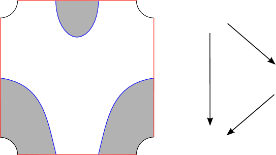
zz at 30 150 \pinlabel11 at 150 150 \pinlabel22 at 150 30 \pinlabel33 at 30 30 \pinlabelx1x_{1} at 120 -15 \pinlabelx2x_{2} at -15 90 \pinlabelx3x_{3} at 70 -15 \pinlabelx1x_{1} at 250 160 \pinlabelx2x_{2} at 340 90 \pinlabelx3x_{3} at 250 20 \pinlabela⁡(ρ2)a(\rho_{2}) at 325 145 \pinlabela⁡(ρ1)a(\rho_{1}) at 325 40 \pinlabel11 at 240 90 \pinlabel[0a⁡(ρ2)100a⁡(ρ1)000]\begin{bmatrix}0&a(\rho_{2})&1\\ 0&0&a(\rho_{1})\\ 0&0&0\\ \end{bmatrix} at 530 90 \endlabellistRefer to caption

Figure 4. An example of a bounded type DD structure. Left: A Heegaard diagram. The domains that contribute to δ\delta are shaded. Center: The type DD structure for the diagram. Right: A matrix representation of the map δ\delta with respect to the given ordering of the generating set. Note that the notation ρi\rho_{i} here comes from the labels on the diagram and carries a different meaning than in Section 3.

So chose an upper triangular differential matrix for MM and let xx be the generator corresponding to the bottommost row of the matrix. Then xx is a cycle, and, now thinking of MM as a left 𝒜\mathcal{A}-module, we have a distinguished triangle

𝒜​ID​(x)​[m⁡(x)]→M→M/𝒜​x,\mathcal{A}I_{D}(x)[m(x)]\to M\to M/\mathcal{A}x,

so [M]=(−1)m⁡(x)​[𝒜​ID​(x)]+[M/𝒜​x][M]=(-1)^{m(x)}[\mathcal{A}I_{D}(x)]+[M/\mathcal{A}x]. The matrix for M/𝒜​xM/\mathcal{A}x is obtained from the matrix for MM by removing the last row and column, hence M/𝒜​xM/\mathcal{A}x is bounded and can be generated by fewer elements than MM, so by hypothesis [M/𝒜​x][M/\mathcal{A}x] is the sum of symbols of elementary projectives. Thus, [M][M] is of that form too. More precisely, applying the distinguished triangle process repeatedly by moving up the matrix, we see that

[M]=∑x∈𝔖⁡(M)(−1)m⁡(x)​[𝒜​ID​(x)].[M]=\sum_{x\in\mathfrak{S}(M)}(-1)^{m(x)}[\mathcal{A}I_{D}(x)].

So far we have shown that K0​(𝒜)K_{0}(\mathcal{A}) is generated (over ℤ\mathbb{Z}) by the symbols of elementary projectives, , i.e. modules of the form 𝒜​I​(𝐬)\mathcal{A}I({\bf s}).

We now switch to the language of modules over 𝒜\mathcal{A}.

The algebra 𝒜=𝒜⁡(𝒵)\mathcal{A}=\mathcal{A}(\mathcal{Z}) has a ℤ\mathbb{Z}-grading given by the total support of an element in H1​(Z,𝐚)H_{1}(Z,\bf{a}), i.e. the sum of the coefficients of the projection from gr′​(a)∈G′​(𝒵)\textrm{gr}^{\prime}(a)\in G^{\prime}(\mathcal{Z}) onto H1​(Z,𝐚)H_{1}(Z,\bf{a}). Since we only work with upward going and horizontal strands, this grading is in fact by non-negative numbers, and the degree 00 part is precisely the ground ring ℐ\mathcal{I}. The part of positive degree, call it 𝒜+\mathcal{A}_{+}, is an augmentation ideal - dividing by it yields ℐ\mathcal{I}. This augmentation map 𝒜→ℐ\mathcal{A}\to\mathcal{I} induces a map of the categories of modules over 𝒜\mathcal{A} and ℐ\mathcal{I} by M↦M/𝒜+​MM\mapsto M/\mathcal{A}_{+}M. More precisely, an 𝒜\mathcal{A}-module homomorphism f:M→Nf:M\to N maps elements of 𝒜+​M\mathcal{A}_{+}M to 𝒜+​N\mathcal{A}_{+}N, so it descends to an ℐ\mathcal{I}-module homomorphism f′:M/𝒜+M→N/𝒜+​Nf^{\prime}:M/\mathcal{A}+M\to N/\mathcal{A}_{+}N. Thus, distinguished triangles in 𝒫⁡(𝒜)\mathcal{P}(\mathcal{A}) are sent by the augmentation map to distinguished triangles in 𝒫⁡(ℐ)\mathcal{P}(\mathcal{I}). So a relation between the symbols of modules in K0​(𝒜)K_{0}(\mathcal{A}) implies a relation between the corresponding symbols in K0​(ℐ)K_{0}(\mathcal{I}).

Note that there is a correspondence between primitive idempotents and elements of Λ∗​(H1​(F,ℤ))\Lambda^{\ast}(H_{1}(F;\mathbb{Z})) given by I⁡(𝐬)→a𝐬I({\bf s})\to a_{{\bf s}}, so we can identify K0​(ℐ)=K0​((ℤ/2)22​k)≅ℤ22​kK_{0}(\mathcal{I})=K_{0}((\mathbb{Z}/2)^{2^{2k}})\cong\mathbb{Z}^{2^{2k}} with Λ∗​(H1​(F,ℤ))\Lambda^{\ast}(H_{1}(F;\mathbb{Z})) via [𝒜​I​(𝐬)]=a𝐬[\mathcal{A}I({\bf s})]=a_{{\bf s}}. Thus,

K0​(𝒜)=Λ∗​(H1​(F,ℤ)).K_{0}(\mathcal{A})=\Lambda^{\ast}(H_{1}(F;\mathbb{Z})).

∎

5. K0K_{0} of Alexander-graded dg modules over 𝒜⁡(𝒵)\mathcal{A}(\mathcal{Z})

In this section, we define a relative 12​ℤ\frac{1}{2}\mathbb{Z}-grading aa on the dg algebra 𝒜⁡(𝒵)\mathcal{A}(\mathcal{Z}), as well as on the left type DD structures and right 𝒜∞\mathcal{A}_{\infty}-modules over 𝒜⁡(𝒵)\mathcal{A}(\mathcal{Z}). We refer to it as Alexander grading, and show that it has properties similar to the Alexander grading on 𝐶𝐹𝐾^\widehat{\mathit{CFK}} for links in closed 33-manifolds. For now we restrict to the case of torus boundary, and define an Alexander grading for 𝐶𝐹𝐷^\widehat{\mathit{CFD}} of knot complements and for 𝐶𝐹𝐴^\widehat{\mathit{CFA}} of knots in the solid torus.

The pointed matched circle 𝒵=𝒵⁡(T2)\mathcal{Z}=\mathcal{Z}(T^{2}) for a torus is depicted in in Figure 5. Four points are matched into two pairs α1\alpha_{1} and α2\alpha_{2}, and divide the circle into the four upward-oriented arcs ρ0\rho_{0}, ρ1\rho_{1}, ρ2\rho_{2}, and ρ3\rho_{3} (not to be confused with the ρi\rho_{i} in Section 3), where ρ0\rho_{0} contains the basepoint zz. The algebra 𝒜⁡(𝒵)\mathcal{A}(\mathcal{Z}) has two idempotents, one for each αi\alpha_{i}, and 66 Reeb elements, coming from the Reeb chords ρ1,ρ2\rho_{1},\rho_{2} and ρ3\rho_{3} (also see [7, Section 11.1]).

Refer to caption
Figure 5. The circle 𝒵\mathcal{Z} in the case of torus boundary

Recall that the unrefined grading on the torus algebra takes values in the group G′G^{\prime} which consists of quadruples (j,r1,r2,r3)(j;r_{1},r_{2},r_{3}), with j∈12​ℤj\in\frac{1}{2}\mathbb{Z}, ri∈ℤr_{i}\in\mathbb{Z}, and jj is an integer if r2r_{2} and r1−r3r_{1}-r_{3} are even. There is also a refined grading by a subgroup GG, different from G⁡(𝒵)G(\mathcal{Z}), which consists of triples (j,q1,q2)(j;q_{1},q_{2}) with j,q1,q2∈12​ℤj,q_{1},q_{2}\in\frac{1}{2}\mathbb{Z} and q1+q2∈ℤq_{1}+q_{2}\in\mathbb{Z}. For the group law on G′G^{\prime} and GG and further details, see [7, Section 11.1].

We have a surjection

G′\displaystyle G^{\prime} ↠H1​(Z,𝐚)\displaystyle\twoheadrightarrow H_{1}(Z,\bf a)
(j,r1,r2,r3)\displaystyle(j;r_{1},r_{2},r_{3}) ↦(r1,r2,r3)\displaystyle\mapsto(r_{1},r_{2},r_{3})

As with the refined grading group G⁡(𝒵)G(\mathcal{Z}), we can think of GG as a ℤ\mathbb{Z} central extension of H1​(T2,12​ℤ)H_{1}(T^{2};\frac{1}{2}\mathbb{Z}). In other words, we have a map

G\displaystyle G →H1​(T2,ℚ)\displaystyle\to H_{1}(T^{2};\mathbb{Q})
(j,q1,q2)\displaystyle(j;q_{1},q_{2}) ↦(q1,q2)\displaystyle\mapsto(q_{1},q_{2})

with image inside 12​ℤ×12​ℤ\frac{1}{2}\mathbb{Z}\times\frac{1}{2}\mathbb{Z} and kernel generated by λ=(1,0,0)\lambda=(1;0,0).

Let KK be a knot in S3S^{3} and let 𝐶𝐹𝐷^​(K,n)\widehat{\mathit{CFD}}(K,n) be a type DD structure for the nn-framed complement S3∖KS^{3}\setminus K. Fix a generator xx and recall that we can choose the sign of the generator BB of π2​(x,x)\pi_{2}(x,x) so that BB does not cover the basepoint zz, and has multiplicities 1,n+1,n1,n+1,n at the regions corresponding to ρ1,ρ2,ρ3\rho_{1},\rho_{2},\rho_{3}, respectively.

We can define the Alexander grading in two ways: by composing gr′\textrm{gr}^{\prime} with map from G′G^{\prime} to 12​ℤ\frac{1}{2}\mathbb{Z}, or by composing gr with a map from the subgroup GG to 12​ℤ\frac{1}{2}\mathbb{Z}. The two maps to 12​ℤ\frac{1}{2}\mathbb{Z} are obtained by composing the two maps above with

H1​(Z,𝐚)\displaystyle H_{1}(Z,\bf a) →12​ℤ\displaystyle\to\textstyle\frac{1}{2}\mathbb{Z}
(r1,r2,r3)\displaystyle(r_{1},r_{2},r_{3}) ↦n+12​r1+n−12​r2+−n−12​r3\displaystyle\mapsto\textstyle{\frac{n+1}{2}r_{1}+\frac{n-1}{2}r_{2}+\frac{-n-1}{2}r_{3}}

and

H1​(T2,ℚ)\displaystyle H_{1}(T^{2};\mathbb{Q}) →12​ℤ\displaystyle\to\textstyle\frac{1}{2}\mathbb{Z}
(q1,q2)\displaystyle(q_{1},q_{2}) ↦n​q1−q2.\displaystyle\mapsto nq_{1}-q_{2}.

The gradings g′​(B)g^{\prime}(B) and g⁡(B)g(B) are in the kernel of the respective maps, so we get maps from the quotients G′/P⁡(x)G^{\prime}/P(x) and G/P⁡(x)G/P(x) to 12​ℤ\frac{1}{2}\mathbb{Z}, i.e. an Alexander grading on 𝐶𝐹𝐷^​(K,n)\widehat{\mathit{CFD}}(K,n) by 12​ℤ\frac{1}{2}\mathbb{Z}, which we denote by aa.

Also note that the two maps commute with the grading maps (i.e. transitioning between GG and G′G^{\prime}), hence the two maps define the same grading on 𝐶𝐹𝐷^​(K,n)\widehat{\mathit{CFD}}(K,n) by 12​ℤ\frac{1}{2}\mathbb{Z}. Note that this grading agrees with the function SS from [7, Equation 11.39].

Next, we define the Alexander grading for a knot in the solid torus. One might like to just add the number of times we pass through the second basepoint of the Heegaard diagram to the Alexander grading above, but we also have to keep track of the homological class of the knot in the solid torus.

Given a 00-framed solid torus and a knot KK in it with homology class [p][p], fix a generator xx of 𝐶𝐹𝐴^​(K)\widehat{\mathit{CFA}}(K), and note that we can choose the generator BB of π2​(x,x)\pi_{2}(x,x) to have multiplicities 0,1,10,1,1 at ρ1,ρ2,ρ3\rho_{1},\rho_{2},\rho_{3} respectively, and to avoid the basepoint zz. This BB covers ww with multiplicity pp: the boundary of BB is a set of complete α\alpha and β\beta circles, and the complete arc α1\alpha_{1}. By capping off all circles with the disks they bound, we get an immersed surface in the solid torus whose boundary is the meridian of the solid torus. In other words, the surface we obtain from BB is homologically equivalent to the disk D2D^{2} (with positive orientation) that the meridian bounds, hence intersects the knot homologically pp any times. Hence, in the Heegaard diagram, BB covers the basepoint ww a total of pp many times.

This time we have the algebra graded by G′×{0}G^{\prime}\times\{0\} or G×{0}G\times\{0\} as subgroups of G′×ℤG^{\prime}\times\mathbb{Z} or G′×ℤG^{\prime}\times\mathbb{Z}, and corresponding maps to H1​(Z,𝐚)×ℤH_{1}(Z,\bf a)\times\mathbb{Z} or H1​(T2,ℚ)×ℤH_{1}(T^{2};\mathbb{Q})\times\mathbb{Z} defined as above on the first factor, and as the identity on the second. Define the Alexander grading aa on the algebra as the composition of these maps with the maps to 12​ℤ\frac{1}{2}\mathbb{Z} given by (r1,r2,r3,d)↦d−p⁡(r2+r3)(r_{1},r_{2},r_{3};d)\mapsto d-p(r_{2}+r_{3}) and (q1,q2,d)↦d−p​q2(q_{1},q_{2};d)\mapsto d-pq_{2} respectively.

The domain BB above has grading of the form g′​(B)=(_,0,1,1,p)g^{\prime}(B)=(\_;0,1,1;p) in G′G^{\prime}, or g⁡(B)=(_,0,1,p)g(B)=(\_;0,1;p) in GG, and the grading on 𝐶𝐹𝐴^​(K)\widehat{\mathit{CFA}}(K) takes values in G′×ℤ/⟨g′​(B)⟩G^{\prime}\times\mathbb{Z}/\langle g^{\prime}(B)\rangle or G×ℤ/⟨g⁡(B)⟩G\times\mathbb{Z}/\langle g(B)\rangle, respectively. The gradings of BB are in the kernels of the maps, so we get well defined maps from the quotients G′×ℤ/⟨g′​(B)⟩G^{\prime}\times\mathbb{Z}/\langle g^{\prime}(B)\rangle and G×ℤ/⟨g⁡(B)⟩G\times\mathbb{Z}/\langle g(B)\rangle to 12​ℤ\frac{1}{2}\mathbb{Z}, and also note that the two maps commute with the grading maps, hence we have a well defined grading on 𝐶𝐹𝐴^​(K)\widehat{\mathit{CFA}}(K), which we also call the Alexander grading and denote by aa.

Note that a 12​ℤ\frac{1}{2}\mathbb{Z}-grading introduces relation (3) in Definition 17, and the Grothendieck group for left type DD structures and right 𝒜∞\mathcal{A}_{\infty}-modules over 𝒜⁡(𝒵)\mathcal{A}(\mathcal{Z}) becomes

K0(𝒜(𝒵)g​r)≅Λ∗(H1(F;ℤ))⊗ℤ[t1/2,t−1/2].K_{0}(\mathcal{A}(\mathcal{Z})_{gr})\cong\Lambda^{\ast}(H_{1}(F;\mathbb{Z}))\otimes\mathbb{Z}[t^{1/2},t^{-1/2}].

6. Tensor products

We first show that as a relative grading, the grading mm defined in Section 3 agrees with the relative Maslov grading for closed manifolds.

Let Y1Y_{1} and Y2Y_{2} be bordered 33-manifolds which agree along their boundary, with Heegaard diagrams ℋ1\mathcal{H}_{1} and ℋ2\mathcal{H}_{2} which can be glued along their boundary 𝒵=∂ℋ1=−∂ℋ2\mathcal{Z}=\partial\mathcal{H}_{1}=-\partial\mathcal{H}_{2} to form a closed Heegaard diagram ℋ=ℋ1∪∂ℋ2\mathcal{H}=\mathcal{H}_{1}\cup_{\partial}\mathcal{H}_{2} representing the closed 33-manifold Y=Y1∪∂Y2Y=Y_{1}\cup_{\partial}Y_{2}. Let 𝔰∈spinc​(Y)\mathfrak{s}\in\mathrm{spin}^{c}(Y), and let 𝔰i=𝔰|Yi\mathfrak{s}_{i}=\mathfrak{s}|_{Y_{i}}.

Let u,v∈𝐶𝐹𝐴^​(ℋ1,𝔰1)u,v\in\widehat{\mathit{CFA}}(\mathcal{H}_{1},\mathfrak{s}_{1}) and x,y∈𝐶𝐹𝐷^​(ℋ2,𝔰2)x,y\in\widehat{\mathit{CFD}}(\mathcal{H}_{2},\mathfrak{s}_{2}) be homogeneous elements with respect to the grading gr, and suppose uu and xx occupy complementary α\alpha-arcs, and so do vv and yy, and u⊠xu\boxtimes x and v⊠yv\boxtimes y are in the same spinc\textrm{spin}^{c} structure 𝔰\mathfrak{s}.

Proposition 22.

Let tt be the relative Maslov grading mod 22 between u⊠xu\boxtimes x and v⊠y∈𝐶𝐹^​(ℋ,𝔰)v\boxtimes y\in\widehat{\mathit{CF}}(\mathcal{H},\mathfrak{s}) (see [7, Theorem 10.42]). Then

[m⁡(u)+m⁡(x)]−[m⁡(v)+m⁡(y)]=t​ mod ​2[m(u)+m(x)]-[m(v)+m(y)]=t\text{\emph{ mod} }2

Recall that 𝐶𝐹𝐴^​(ℋ1,𝔰1)\widehat{\mathit{CFA}}(\mathcal{H}_{1},\mathfrak{s}_{1}) is graded by P1​(x1)\G⁡(𝒵)P_{1}(x_{1})\backslash G(\mathcal{Z}), where x1∈𝔖⁡(ℋ1,𝔰1)x_{1}\in\mathfrak{S}(\mathcal{H}_{1},\mathfrak{s}_{1}) is a chosen base generator, and P1​(x1)P_{1}(x_{1}) is the image of π2​(x1,x1)\pi_{2}(x_{1},x_{1}) in G⁡(𝒵)G(\mathcal{Z}). Similarly, 𝐶𝐹𝐷^​(ℋ2,𝔰2)\widehat{\mathit{CFD}}(\mathcal{H}_{2},\mathfrak{s}_{2}) is graded by G⁡(𝒵)/R⁡(P2​(x2))G(\mathcal{Z})/R(P_{2}(x_{2})), where x2∈𝔖⁡(ℋ2,𝔰2)x_{2}\in\mathfrak{S}(\mathcal{H}_{2},\mathfrak{s}_{2}) is a chosen base generator and P2​(x2)P_{2}(x_{2}) is the image of π2​(x2,x2)\pi_{2}(x_{2},x_{2}) in G⁡(𝒵)G(\mathcal{Z}). Recall that the map ff from Section 3 maps any element of P1​(x1)P_{1}(x_{1}) or R​(P2​(x2))R(P_{2}(x_{2})) to zero.

By [7, Theorem 10.42],

gr⊠​(u⊠x)=λt​gr⊠​(v⊠y)∈P1​(x1)\G⁡(𝒵)/R⁡(P2​(x2)).\textrm{gr}^{\boxtimes}(u\boxtimes x)=\lambda^{t}\textrm{gr}^{\boxtimes}(v\boxtimes y)\in P_{1}(x_{1})\backslash G(\mathcal{Z})/R(P_{2}(x_{2})).

This means that if we fix representatives gu,gv,gx,gy∈G⁡(𝒵)g_{u},g_{v},g_{x},g_{y}\in G(\mathcal{Z}) so that [gu]=gr​(u)∈P1​(x1)\G⁡(𝒵)[g_{u}]=\textrm{gr}(u)\in P_{1}(x_{1})\backslash G(\mathcal{Z}), etc., then

[gu​gx]=[λt​gv​gy]∈P1​(x1)\G⁡(𝒵)/R⁡(P2​(x2)).[g_{u}g_{x}]=[\lambda^{t}g_{v}g_{y}]\in P_{1}(x_{1})\backslash G(\mathcal{Z})/R(P_{2}(x_{2})).

Then there exist h1∈P1​(x1)h_{1}\in P_{1}(x_{1}) and h2∈R⁡(P2​(x2))h_{2}\in R(P_{2}(x_{2})), such that

h1​gu​gx​h2=λt​gv​gy∈G⁡(𝒵).h_{1}g_{u}g_{x}h_{2}=\lambda^{t}g_{v}g_{y}\in G(\mathcal{Z}).

Applying ff to both sides, we see that

f⁡(h1​gu​gx​h2)=f⁡(λt​gv​gy),f(h_{1}g_{u}g_{x}h_{2})=f(\lambda^{t}g_{v}g_{y}),

so

0\displaystyle 0 =f⁡(h1​gu​gx​h2)−f⁡(λt​gv​gy)\displaystyle=f(h_{1}g_{u}g_{x}h_{2})-f(\lambda^{t}g_{v}g_{y})
=f⁡(h1)+f⁡(gu)+f⁡(gx)+f⁡(h2)−t​f​(λ)−f⁡(gv)−f⁡(gy)\displaystyle=f(h_{1})+f(g_{u})+f(g_{x})+f(h_{2})-tf(\lambda)-f(g_{v})-f(g_{y})
=f⁡(gu)+f⁡(gx)−t−f⁡(gv)−f⁡(gy)\displaystyle=f(g_{u})+f(g_{x})-t-f(g_{v})-f(g_{y})
=f¯​(gr​(u))+f¯​(gr​(x))−t−f¯​(gr​(v))−f¯​(gr​(y))\displaystyle=\overline{f}(\textrm{gr}(u))+\overline{f}(\textrm{gr}(x))-t-\overline{f}(\textrm{gr}(v))-\overline{f}(\textrm{gr}(y))
=m⁡(u)+m⁡(x)−t−m⁡(v)−m⁡(y).∎\displaystyle=m(u)+m(x)-t-m(v)-m(y).\qed

A similar statement can be made about the Alexander grading on the manifolds studied in Section 5. Let ℋ1\mathcal{H}_{1} be a Heegaard diagram for a knot in a 00-framed solid torus (S1×D2,C)(S^{1}\times D^{2},C), and let ℋ2\mathcal{H}_{2} be a Heegaard diagram for a 00-framed knot complement (S3∖K,0)(S^{3}\setminus K,0), so that ℋ=ℋ1∪∂ℋ2\mathcal{H}=\mathcal{H}_{1}\cup_{\partial}\mathcal{H}_{2} is a Heegaard diagram for (S3,KC)(S^{3},K_{C}). Recall that there is only one spinc\textrm{spin}^{c} structure for each of the bordered manifolds and for S3S^{3}. Also recall that for knots, we enhance the grading group GG to G×ℤG\times\mathbb{Z}, and in this case 𝐶𝐹𝐴^​(ℋ1)\widehat{\mathit{CFA}}(\mathcal{H}_{1}) is graded by the coset space ⟨hA⟩\G\langle h_{A}\rangle\backslash G, and 𝐶𝐹𝐷^​(ℋ2)\widehat{\mathit{CFD}}(\mathcal{H}_{2}) is graded by a coset space G/⟨hD⟩G/\langle h_{D}\rangle, where ⟨hA⟩\langle h_{A}\rangle and ⟨hD⟩\langle h_{D}\rangle are the images in GG of the the groups of periodic domains of ℋ1\mathcal{H}_{1} and ℋ2\mathcal{H}_{2}. Every element of the double-coset space ⟨hA⟩\G/⟨hD⟩\langle h_{A}\rangle\backslash G/\langle h_{D}\rangle has a representative of the form (j,0,0,d)(j;0,0;d), where j,d∈ℤj,d\in\mathbb{Z}, so we can think of 𝐶𝐹𝐴^​(ℋ1)⊠𝐶𝐹𝐷^​(ℋ2)\widehat{\mathit{CFA}}(\mathcal{H}_{1})\boxtimes\widehat{\mathit{CFD}}(\mathcal{H}_{2}) as graded by ℤ×ℤ\mathbb{Z}\times\mathbb{Z}. The second factor, i.e. the number dd, is in fact the relative Alexander grading for knot Floer homology. For more detail on these facts, we refer the reader to the the discussion preceding [7, Theorem 11.21], and the computation example in [7, Section 11.9].

Proposition 23.

Let u,v∈𝐶𝐹𝐴^​(ℋ1)u,v\in\widehat{\mathit{CFA}}(\mathcal{H}_{1}) and x,y∈𝐶𝐹𝐷^​(ℋ2)x,y\in\widehat{\mathit{CFD}}(\mathcal{H}_{2}) be homogeneous elements with respect to the grading gr, and suppose uu and xx occupy complementary α\alpha-arcs, and so do vv and yy. Let AA be the relative Alexander grading between u⊠xu\boxtimes x and v⊠y∈𝐶𝐹𝐾^​(ℋ)v\boxtimes y\in\widehat{\mathit{CFK}}(\mathcal{H}). Then

(a⁡(u)+p⋅a⁡(x))−(a⁡(v)+p⋅a⁡(y))=A(a(u)+p\cdot a(x))-(a(v)+p\cdot a(y))=A

The Maslov component does not affect the computation, so we leave it blank. Recall that in this 00-framed case we can assume that hAh_{A} has form (_,0,1,p)(\_;0,1;p) and hDh_{D} has form (_,1,0,0)(\_;1,0;0).

Fix representatives

gu\displaystyle g_{u} =(_,pu,qu,du),\displaystyle=(\_;p_{u},q_{u};d_{u}),
gv\displaystyle g_{v} =(_,pv,qv,dv),\displaystyle=(\_;p_{v},q_{v};d_{v}),
gx\displaystyle g_{x} =(_,px,qx,dx),\displaystyle=(\_;p_{x},q_{x};d_{x}),
gy\displaystyle g_{y} =(_,py,qy,dy)\displaystyle=(\_;p_{y},q_{y};d_{y})

in GG so that [gu]=gr​(u)∈⟨hA⟩\G[g_{u}]=\textrm{gr}(u)\in\langle h_{A}\rangle\backslash G, etc. Then

[gu​gx]=[hA−qu−qx​gu​gx​hD−pu−px]=[(_,0,0,du−p​qu−p​qx)],[g_{u}g_{x}]=[h_{A}^{-q_{u}-q_{x}}g_{u}g_{x}h_{D}^{-p_{u}-p_{x}}]=[(\_;0,0;d_{u}-pq_{u}-pq_{x})],
[gv​gy]=[hA−qv−qy​gv​gy​hD−pv−py]=[(_,0,0,dv−p​qv−p​qy)],[g_{v}g_{y}]=[h_{A}^{-q_{v}-q_{y}}g_{v}g_{y}h_{D}^{-p_{v}-p_{y}}]=[(\_;0,0;d_{v}-pq_{v}-pq_{y})],

and so A=A⁡(u⊠x)−A⁡(v⊠y)=(du−p​qu−p​qx)−(dv−p​qv−p​qy)A=A(u\boxtimes x)-A(v\boxtimes y)=(d_{u}-pq_{u}-pq_{x})-(d_{v}-pq_{v}-pq_{y}), which equals precisely (a⁡(u)+p⋅a⁡(x))−(a⁡(v)+p⋅a⁡(y))(a(u)+p\cdot a(x))-(a(v)+p\cdot a(y)). ∎

Now we define a product operation on Λ∗​H1​(F,ℤ)\Lambda^{\ast}H_{1}(F;\mathbb{Z}). Define an inner product on the vector space H1​(F,ℤ)H_{1}(F;\mathbb{Z}) by

⟨ai,aj⟩={1if i=j0otherwise,\langle a_{i},a_{j}\rangle=\left\{\begin{array}[]{ll}1&\textrm{if $i=j$}\\ 0&\textrm{otherwise,}\end{array}\right.

i.e. so that {a1,…,a2​k}\{a_{1},\ldots,a_{2k}\} is an orthonormal basis. This extends to an inner product on Λn​H1​(F,ℤ)\Lambda^{n}H_{1}(F;\mathbb{Z}) by

⟨v1∧⋯∧vn,w1∧⋯∧wn⟩=det(⟨vi,wj⟩)\langle v_{1}\wedge\cdots\wedge v_{n},w_{1}\wedge\cdots\wedge w_{n}\rangle=\det(\langle v_{i},w_{j}\rangle)

and {aJ||J|=n}\{a_{J}||J|=n\} is an orthonormal basis for Λn​H1​(F,ℤ)\Lambda^{n}H_{1}(F;\mathbb{Z}). We define an operation ⋅\cdot on Λ∗​H1​(F,ℤ)\Lambda^{\ast}H_{1}(F;\mathbb{Z}) by

x⋅y:=⟨x1,y1⟩+⟨x2,y2⟩+⋯+⟨x2​k,y2​k⟩,x\cdot y:=\langle x_{1},y_{1}\rangle+\langle x_{2},y_{2}\rangle+\cdots+\langle x_{2k},y_{2k}\rangle,

where xix_{i} and yiy_{i} are the Λi\Lambda^{i} components of xx and yy, respectively.

For the first part, M⊠NM\boxtimes N inherits a ℤ/2\mathbb{Z}/2 grading from MM and NN by m⁡(x⊠y)=m⁡(x)+m⁡(y)m(x\boxtimes y)=m(x)+m(y). We have

[M]⋅[N]\displaystyle[M]\cdot[N] =∑x∈𝔖⁡(M)(−1)m⁡(x)​h​(x)⋅∑y∈𝔖⁡(N)(−1)m⁡(y)​h​(y)\displaystyle=\sum_{x\in\mathfrak{S}(M)}(-1)^{m(x)}h(x)\cdot\sum_{y\in\mathfrak{S}(N)}(-1)^{m(y)}h(y)
=(∑𝐬⊂[2​k]a𝐬​∑x∈𝔖⁡(M),h⁡(x)=a𝐬(−1)m⁡(x))⋅(∑𝐭⊂[2​k]a𝐭​∑y∈𝔖⁡(N),h⁡(y)=a𝐭(−1)m⁡(y))\displaystyle=\left(\sum_{{\bf s}\subset[2k]}a_{{\bf s}}\sum_{x\in\mathfrak{S}(M),h(x)=a_{{\bf s}}}(-1)^{m(x)}\right)\cdot\left(\sum_{{\bf t}\subset[2k]}a_{{\bf t}}\sum_{y\in\mathfrak{S}(N),h(y)=a_{{\bf t}}}(-1)^{m(y)}\right)
=∑𝐬,𝐭∈[2​k]|𝐬|=|𝐭|⟨a𝐬,a𝐭⟩​∑x∈𝔖⁡(M),h⁡(x)=a𝐬y∈𝔖⁡(N),h⁡(y)=a𝐭(−1)m⁡(x)​(−1)m⁡(y)\displaystyle=\sum_{\begin{subarray}{c}{\bf s},{\bf t}\in[2k]\\ |{\bf s}|=|{\bf t}|\end{subarray}}\langle a_{{\bf s}},a_{{\bf t}}\rangle\sum_{\begin{subarray}{c}x\in\mathfrak{S}(M),h(x)=a_{{\bf s}}\\ y\in\mathfrak{S}(N),h(y)=a_{{\bf t}}\end{subarray}}(-1)^{m(x)}(-1)^{m(y)}
=∑x∈𝔖⁡(M),y∈𝔖⁡(N)h⁡(x)=a𝐬=h⁡(y)(−1)m⁡(x)+m⁡(y)\displaystyle=\sum_{\begin{subarray}{c}x\in\mathfrak{S}(M),y\in\mathfrak{S}(N)\\ h(x)=a_{{\bf s}}=h(y)\end{subarray}}(-1)^{m(x)+m(y)}
=∑x⊠y(−1)m⁡(x)+m⁡(y)\displaystyle=\sum_{x\boxtimes y}(-1)^{m(x)+m(y)}
=χ⁡(M⊠N).\displaystyle=\chi(M\boxtimes N).

The second part is the specialization of the first part to 𝐶𝐹𝐴^\widehat{\mathit{CFA}} and 𝐶𝐹𝐷^\widehat{\mathit{CFD}} with the grading mm defined in Section 3 and 𝐶𝐹^\widehat{\mathit{CF}} graded by the Maslov grading. We remark that [𝐶𝐹𝐷^][\widehat{\mathit{CFD}}] and [𝐶𝐹𝐴^][\widehat{\mathit{CFA}}] are elements of Λk​H1​(F,ℤ)\Lambda^{k}H_{1}(F;\mathbb{Z}). The last step in the above equation follows, up to an overall sign for each spinc\mathrm{spin}^{c} structure, from Proposition 22. ∎

This is the Alexander-graded version of Theorem 2. Recall that homology solid tori have a unique spinc\mathrm{spin}^{c} structure. For ℋ1\mathcal{H}_{1} and ℋ2\mathcal{H}_{2} as in Proposition 23,

[𝐶𝐹𝐴^​(ℋ1)]\displaystyle[\widehat{\mathit{CFA}}(\mathcal{H}_{1})] =∑x∈𝔖⁡(ℋ1)IA​(x)=ι0(−1)m⁡(x)​ta⁡(x)​a1+∑x∈𝔖⁡(ℋ1)IA​(x)=ι1(−1)m⁡(x)​ta⁡(x)​a2\displaystyle=\sum_{\begin{subarray}{c}x\in\mathfrak{S}(\mathcal{H}_{1})\\ I_{A}(x)=\iota_{0}\end{subarray}}(-1)^{m(x)}t^{a(x)}a_{1}+\sum_{\begin{subarray}{c}x\in\mathfrak{S}(\mathcal{H}_{1})\\ I_{A}(x)=\iota_{1}\end{subarray}}(-1)^{m(x)}t^{a(x)}a_{2}
[𝐶𝐹𝐷^​(ℋ2)]\displaystyle[\widehat{\mathit{CFD}}(\mathcal{H}_{2})] =∑y∈𝔖⁡(ℋ2)ID​(y)=ι0(−1)m⁡(y)​ta⁡(y)​a1+∑y∈𝔖⁡(ℋ2)ID​(y)=ι1(−1)m⁡(y)​ta⁡(y)​a2.\displaystyle=\sum_{\begin{subarray}{c}y\in\mathfrak{S}(\mathcal{H}_{2})\\ I_{D}(y)=\iota_{0}\end{subarray}}(-1)^{m(y)}t^{a(y)}a_{1}+\sum_{\begin{subarray}{c}y\in\mathfrak{S}(\mathcal{H}_{2})\\ I_{D}(y)=\iota_{1}\end{subarray}}(-1)^{m(y)}t^{a(y)}a_{2}.

We multiply out and see that [𝐶𝐹𝐴^​(ℋ1)]⋅[𝐶𝐹𝐷^​(ℋ2)][\widehat{\mathit{CFA}}(\mathcal{H}_{1})]\cdot[\widehat{\mathit{CFD}}(\mathcal{H}_{2})] equals

∑x∈𝔖⁡(ℋ1),y∈𝔖⁡(ℋ2)IA​(x)=ι0=ID​(y)\displaystyle\sum_{\begin{subarray}{c}x\in\mathfrak{S}(\mathcal{H}_{1}),y\in\mathfrak{S}(\mathcal{H}_{2})\\ I_{A}(x)=\iota_{0}=I_{D}(y)\end{subarray}} (−1)m⁡(x)+m⁡(y)​ta⁡(x)+p​a​(y)+∑x∈𝔖⁡(ℋ1),y∈𝔖⁡(ℋ2)IA​(x)=ι1=ID​(y)(−1)m⁡(x)+m⁡(y)​ta⁡(x)+p​a​(y)\displaystyle(-1)^{m(x)+m(y)}t^{a(x)+pa(y)}+\sum_{\begin{subarray}{c}x\in\mathfrak{S}(\mathcal{H}_{1}),y\in\mathfrak{S}(\mathcal{H}_{2})\\ I_{A}(x)=\iota_{1}=I_{D}(y)\end{subarray}}(-1)^{m(x)+m(y)}t^{a(x)+pa(y)}
=∑x∈𝔖⁡(ℋ1),y∈𝔖⁡(ℋ2)x⊠y≠0(−1)m⁡(x)+m⁡(y)​ta⁡(x)+p​a​(y)\displaystyle=\sum_{\begin{subarray}{c}x\in\mathfrak{S}(\mathcal{H}_{1}),y\in\mathfrak{S}(\mathcal{H}_{2})\\ x\boxtimes y\neq 0\end{subarray}}(-1)^{m(x)+m(y)}t^{a(x)+pa(y)}
=∑x∈𝔖⁡(ℋ1),y∈𝔖⁡(ℋ2)x⊠y≠0(−1)M⁡(x⊠y)​tA⁡(x⊠y)\displaystyle=\sum_{\begin{subarray}{c}x\in\mathfrak{S}(\mathcal{H}_{1}),y\in\mathfrak{S}(\mathcal{H}_{2})\\ x\boxtimes y\neq 0\end{subarray}}(-1)^{M(x\boxtimes y)}t^{A(x\boxtimes y)}
=±tk​χ​(𝐶𝐹𝐾^​(KC))\displaystyle=\pm t^{k}\chi(\widehat{\mathit{CFK}}(K_{C}))

Gluing a Heegaard diagram for the unknot in the 00-framed solid torus with one generator (see [12, Section 3]) to a diagram for (S3∖K,0)(S^{3}\setminus K,0) shows that the a1a_{1} component of [𝐶𝐹𝐷^​(S3∖K,0)][\widehat{\mathit{CFD}}(S^{3}\setminus K,0)] is χ⁡(𝐶𝐹𝐾^​(K))=ΔK​(t)\chi(\widehat{\mathit{CFK}}(K))=\Delta_{K}(t). Similarly, gluing a diagram with one generator for the 00-framed complement of the unknot to a diagram for C↪S1×D2C\hookrightarrow S^{1}\times D^{2} in a 00-framed S1×D2S^{1}\times D^{2} shows that the a1a_{1} component of [𝐶𝐹𝐴^​(S1×D2,C)][\widehat{\mathit{CFA}}(S^{1}\times D^{2},C)] is χ⁡(𝐶𝐹𝐾^​(C))=ΔC​(t).\chi(\widehat{\mathit{CFK}}(C))=\Delta_{C}(t).

Proving that the a2a_{2} component of [𝐶𝐹𝐷^​(S3∖K,0)][\widehat{\mathit{CFD}}(S^{3}\setminus K,0)] vanishes requires a different argument. Say rank⁡𝐻𝐹𝐾^​(S3,K)=n\rank\widehat{\mathit{HFK}}(S^{3},K)=n and assume we have a basis {x0,…,x2​n}\{x_{0},\ldots,x_{2n}\} for 𝐶𝐹𝐾−​(K)\mathit{CFK}^{-}(K) which is both horizontally and vertically simplified. We illustrate 𝐶𝐹𝐾−​(K)\mathit{CFK}^{-}(K) on the (U,A)(U,A) lattice as in [12, Section 3]. Recall this means we have 2​n+12n+1 points {ξ0,…,ξ2​n}\{\xi_{0},\ldots,\xi_{2n}\} representing the basis, and a vertical (respectively horizontal) arrow from xix_{i} to xjx_{j} of length ll is represented by a vertical (respectively horizontal) arrow of length ll pointing down (respectively to the left) staring at ξi\xi_{i} and ending at ξj\xi_{j}. Note that there is at most one vertical and at most one horizontal arrow starting or ending at each basis element, and there is a unique element ξv\xi^{v} with no in-coming or out-going vertical arrow, and a unique element ξh\xi^{h} with no in-coming or out-going horizontal arrow. See Figure 6.

Recall that we can obtain 𝐶𝐹𝐷^​(S3∖K,0)\widehat{\mathit{CFD}}(S^{3}\setminus K,0) by replacing arrows with chains of coefficient maps, and adding one more chain from ξv\xi^{v} to ξh\xi^{h}, called the unstable chain.

Choose ι0\iota_{0} to be the base idempotent, and define ψ⁡(ι1)=(12,1,0,0)∈G′​(4)\psi(\iota_{1})=(\frac{1}{2};1,0,0)\in G^{\prime}(4). This refinement give rise to a G⁡(𝒵)G(\mathcal{Z}) grading, and hence to a ℤ/2\mathbb{Z}/2 grading mm. With this choice, we list the relative (m,a)(m,a) gradings of a horizontal chain of length ll, a vertical chain of length ll, and the unstable chain when τ⁡(K)=0\tau(K)=0, τ⁡(K)>0\tau(K)>0, and τ⁡(K)<0\tau(K)<0, in this order.

(0,0)\textstyle{(0,0)\ignorespaces\ignorespaces\ignorespaces\ignorespaces}D1\scriptstyle{D_{1}}(0,−12)\textstyle{(0,-\frac{1}{2})}(0,−32)\textstyle{(0,-\frac{3}{2})\ignorespaces\ignorespaces\ignorespaces\ignorespaces}D23\scriptstyle{D_{23}}…\textstyle{\dots\ignorespaces\ignorespaces\ignorespaces\ignorespaces}D23\scriptstyle{D_{23}}(0,12−l)\textstyle{(0,\frac{1}{2}-l)\ignorespaces\ignorespaces\ignorespaces\ignorespaces}D23\scriptstyle{D_{23}}(1,−l)\textstyle{(1,-l)\ignorespaces\ignorespaces\ignorespaces\ignorespaces}D123\scriptstyle{D_{123}}(0,0)\textstyle{(0,0)\ignorespaces\ignorespaces\ignorespaces\ignorespaces}D3\scriptstyle{D_{3}}(0,12)\textstyle{\ignorespaces\ignorespaces\ignorespaces\ignorespaces(0,\frac{1}{2})}D23\scriptstyle{D_{23}}(0,32)\textstyle{(0,\frac{3}{2})\ignorespaces\ignorespaces\ignorespaces\ignorespaces}D23\scriptstyle{D_{23}}…\textstyle{\dots\ignorespaces\ignorespaces\ignorespaces\ignorespaces}D23\scriptstyle{D_{23}}(0,l−12)\textstyle{(0,l-\frac{1}{2})\ignorespaces\ignorespaces\ignorespaces\ignorespaces}D2\scriptstyle{D_{2}}(1,l)\textstyle{(1,l)}(0,0)\textstyle{(0,0)\ignorespaces\ignorespaces\ignorespaces\ignorespaces}D12\scriptstyle{D_{12}}(0,0)\textstyle{(0,0)}        (0,0)\textstyle{(0,0)\ignorespaces\ignorespaces\ignorespaces\ignorespaces}D1\scriptstyle{D_{1}}(0,−12)\textstyle{(0,-\frac{1}{2})}(0,−32)\textstyle{(0,-\frac{3}{2})\ignorespaces\ignorespaces\ignorespaces\ignorespaces}D23\scriptstyle{D_{23}}…\textstyle{\dots\ignorespaces\ignorespaces\ignorespaces\ignorespaces}D23\scriptstyle{D_{23}}(0,12−2​τ)\textstyle{(0,\frac{1}{2}-2\tau)\ignorespaces\ignorespaces\ignorespaces\ignorespaces}D23\scriptstyle{D_{23}\phantom{123}}(0,−2​τ)\textstyle{\ignorespaces\ignorespaces\ignorespaces\ignorespaces(0,-2\tau)}D3\scriptstyle{D_{3}}(0,0)\textstyle{(0,0)\ignorespaces\ignorespaces\ignorespaces\ignorespaces}D123\scriptstyle{D_{123}}(1,12)\textstyle{(1,\frac{1}{2})\ignorespaces\ignorespaces\ignorespaces\ignorespaces}D23\scriptstyle{D_{23}}(1,32)\textstyle{(1,\frac{3}{2})\ignorespaces\ignorespaces\ignorespaces\ignorespaces}D23\scriptstyle{D_{23}}…\textstyle{\dots\ignorespaces\ignorespaces\ignorespaces\ignorespaces}D23\scriptstyle{D_{23}\phantom{1234}}(1,−2​τ−12)\textstyle{(1,-2\tau-\frac{1}{2})\ignorespaces\ignorespaces\ignorespaces\ignorespaces}D2\scriptstyle{D_{2}}(0,−2​τ)\textstyle{(0,-2\tau)}

We plot the chains on the (U,A)(U,A) coordinate system so that the grading aa of a generator with coordinates (x,y)(x,y) is given by x−yx-y. Draw each chain corresponding to a vertical or horizontal arrow also as a vertical or horizontal chain, respectively, and represent coefficient maps between a generator in ι0\iota_{0} and a generator in ι1\iota_{1} by arrows of length 12\frac{1}{2}, and coefficient maps between two generators in ι1\iota_{1} by arrows of length one. The choice for the unstable chain depends on τ⁡(K)\tau(K).

Case 1: τ⁡(K)=0\tau(K)=0. Ignore the D12D_{12} map, and identify ξv\xi^{v} and ξh\xi^{h} if they are not the same basis element. Note this may not result in the correct model for 𝐶𝐹𝐷^​(S3∖K,0)\widehat{\mathit{CFD}}(S^{3}\setminus K,0), but the information about the ι1\iota_{1} elements is intact, which is all we are interested in.

Case 2: τ⁡(K)>0\tau(K)>0.

Note that in this case ξv\xi^{v} is τ⁡(K)\tau(K) units above and τ⁡(K)\tau(K) units to the left of ξh\xi^{h}. Draw the unstable chain in an LL-shape, as follows. Starting at ξv\xi^{v}, represent the first coefficient map by a vertical arrow of length 12\frac{1}{2}, so that the first ι1\iota_{1} element is half a unit below ξv\xi^{v}. Proceed downwards, drawing the D12D_{12} maps to have length one, until half the ι1\iota_{1} elements have been plotted. Repeat the process for the other half, starting at ξh\xi^{h} and going to the left. Connect the middle two elements by a straight arrow to represent the coefficient map between them.

Case 3: τ⁡(K)<0\tau(K)<0.

Here ξv\xi^{v} is |τ⁡(K)||\tau(K)| units below and |τ⁡(K)||\tau(K)| units to the right of ξh\xi^{h}. Rotate the construction for Case 2 by 180∘180^{\circ}.

Figure 6 illustrates the above description with a couple of examples.

Note that each element lies on a line LtL_{t} of slope 11 passing through (t,0)(t,0), for some t∈12​ℤt\in\frac{1}{2}\mathbb{Z}. For ι0\iota_{0} elements t∈ℤt\in\mathbb{Z}, and for ι1\iota_{1} elements t∈ℤ+12t\in\mathbb{Z}+\frac{1}{2}. If a⁡(x)−a⁡(y)=t∈12​ℤa(x)-a(y)=t\in\frac{1}{2}\mathbb{Z}, then the line through xx is tt units above the line through yy.

Let GG be the graph on vertices ξ0,…,ξ2​n\xi_{0},\ldots,\xi_{2n} and edges the 2​n+12n+1 chains (note that if τ⁡(K)=0\tau(K)=0 we may have only 2​n2n vertices and 2​n2n edges), embedded as above. Every vertex has degree 22, so GG is a union of cycles. Endow edges with the orientation induced by the horizontal and vertical arrows for 𝐶𝐹𝐾−\mathit{CFK}^{-}, and orient the edge corresponding to the unstable chain to start at ξv\xi^{v} and end at ξh\xi^{h}.

Rotate the plane clockwise by 45∘45^{\circ}, so that the lines LtL_{t} are now horizontal, and smoothen GG locally at the vertices, so we can think of it as an immersion of a union of circles. The vertices now comprise the local minima, local maxima, and the points with vertical tangents of the immersion. A vertex v≠ξv,ξhv\neq\xi^{v},\xi^{h} is a local maximum if it has an incoming horizontal edge and an outgoing vertical edge, and a local minimum if it has an incoming vertical edge and an outgoing horizontal edge. The vertex ξv\xi^{v} is a local maximum if it has an incoming horizontal edge and τ⁡(K)≥0\tau(K)\geq 0, and a local minimum if it has an outgoing horizontal edge and τ⁡(K)≤0\tau(K)\leq 0. Otherwise it has a vertical tangent. Similarly, ξh\xi^{h} is a local maximum if it has an outgoing vertical edge and τ⁡(K)≤0\tau(K)\leq 0, and a local minimum if it has an incoming vertical edge and τ⁡(K)≥0\tau(K)\geq 0. Note that this covers the case when ξv=ξh\xi^{v}=\xi^{h}.

\labellist\pinlabel

ξv\xi^{v} at 12 575 \pinlabelξh\xi^{h} at 170 414 \pinlabelξh\xi^{h} at 330 567 \pinlabelξv\xi^{v} at 430 440 \endlabellistRefer to caption

Figure 6. Two examples of the graphical interpretation of 𝐶𝐹𝐾−\mathit{CFK}^{-} and 𝐶𝐹𝐷^\widehat{\mathit{CFD}}. Left: The (3,4)(3,4) torus knot (τ=3\tau=3). Right: the (2,−1)(2,-1) cable of the left-handed trefoil (τ=−2\tau=-2). On top are the models for 𝐶𝐹𝐾−\mathit{CFK}^{-}, below are the models for 𝐶𝐹𝐷^\widehat{\mathit{CFD}}, with dashed unstable chain, and on the bottom are the rotated, smoothened graphs. Red and black represent opposite mm gradings.

Tracing the ι1\iota_{1} elements along a connected component of GG, observe that the mm grading changes exactly when passing through a local maximum or minimum. On the other hand, think of a connected component as an immersed circle, ignore the orientations of the edges, and fix an orientation for the circle. The derivative of the height function changes sign exactly at the local maxima or minima, so two ι1\iota_{1} elements have the same mm grading exactly when the derivatives of the height function at their coordinates have the same sign. For any t∈ℤ+12t\in\mathbb{Z}+\frac{1}{2}, the line LtL_{t} crosses GG away from any local minima and maxima, and the oriented intersection number of LtL_{t} and GG is zero, since GG consists of immersed circles. This means that half the intersection points have positive derivative, and the other half have negative derivative (see Figure 6). In other words, half of the ι1\iota_{1} elements of a given aa grading have mm grading 0, and the other half have mm grading 11, and so they cancel each other out in the summation for [𝐶𝐹𝐷^​(S3,K),0][\widehat{\mathit{CFD}}(S^{3},K),0], i.e.

∑x∈𝔖⁡(𝐶𝐹𝐷^​(S3∖K,0)),ID​(x)=ι1(−1)m⁡(x)​ta⁡(x)=0.\sum_{x\in\mathfrak{S}(\widehat{\mathit{CFD}}(S^{3}\setminus K,0)),I_{D}(x)=\iota_{1}}(-1)^{m(x)}t^{a(x)}=0.

In other words, the a2a_{2} component of [𝐶𝐹𝐷^​(S3∖K,0)][\widehat{\mathit{CFD}}(S^{3}\setminus K,0)] is zero.

Last, we show that we do not in fact need the assumption that we have a basis which is both vertically and horizontally simplified.

Let Ξ={ξ0,…,ξ2​n}\Xi=\{\xi_{0},\ldots,\xi_{2n}\} be the plot of a vertically simplified basis with ξv\xi^{v} in position (0,τ)(0,\tau), and let H={η0,…,η2​n}H=\{\eta_{0},\ldots,\eta_{2n}\} be the plot of a horizontally simplified basis with ηh\eta^{h} in position (τ,0)(\tau,0). Also plot the vertical and horizontal chains.

The symmetries of 𝐶𝐹𝐾∞\mathit{CFK}^{\infty} discussed in [10, Section 3.5] imply that when we have a reduced complex, the vertical and horizontal complexes are isomorphic as graded, filtered complexes. The change of basis for this isomorphism may not be a bijection, and in fact may not even map generators to homogeneous linear combinations of generators, but since the isomorphism preserves gradings and filtrations, we may deduce that the number of elements of Ξ\Xi in position (x,y)(x,y) with given Maslov grading is the same as the number of elements of HH with the same grading in position (y,x)(y,x).

In addition, the symmetry

𝐻𝐹𝐾^i​(K,j)≅𝐻𝐹𝐾^i−2​j​(K,−j)\widehat{\mathit{HFK}}_{i}(K,j)\cong\widehat{\mathit{HFK}}_{i-2j}(K,-j)

implies that there is the same number of elements of Ξ\Xi with given parity of the Maslov grading in position (x,y)(x,y), as in position (y,x)(y,x).

Since the grading mm agrees with the Maslov grading, by combining the two symmetries, we see that for a given mm grading (00 or 11) there the number of elements of Ξ\Xi of that grading in a given position (x,y)(x,y) equals the number of elements HH of the same grading in the same position. In other words, we can find a bijection b:H→Ξb:H\to\Xi that preserves coordinates and also preserves the mm grading. Identify the two bases under this bijection, i.e. think of a horizontal chain from ηi\eta_{i} to ηj\eta_{j}, as a horizontal chain from b⁡(ηi)b(\eta_{i}) to b⁡(ηj)b(\eta_{j}), and think of the unstable chain as going from ξv\xi^{v} to b⁡(ηh)b(\eta^{h}). While the result of this identification may not represent 𝐶𝐹𝐷^​(S3∖K,0)\widehat{\mathit{CFD}}(S^{3}\setminus K,0), it has the same graphical structure that we already analyzed in the case of a basis which is simultaneously horizontally and vertically simplified. The bigradings on the chains when moving along a connected component of the graph obey the same rules as before, since bb respects the mm grading, and by [12, Lemma 3.2.5] the aa grading of any element is specified by its coordinates. This allows is to make the same cancelation argument as before. ∎

7. A ℤ/2\mathbb{Z}/2 grading via intersection signs

In Section 3 we defined a ℤ/2\mathbb{Z}/2 differential grading mm on the surface algebra 𝒜⁡(𝒵)\mathcal{A}(\mathcal{Z}) and the left or right modules over it, and showed that it agrees with the Maslov grading after tensoring. For the algebra, this grading was defined as a composition of the G⁡(𝒵)G(\mathcal{Z}) grading from [7] with a homomorphism from G⁡(𝒵)G(\mathcal{Z}) to ℤ/2\mathbb{Z}/2; for the modules, it was defined as a composition of the G⁡(𝒵)G(\mathcal{Z})-set grading with a quotient of the homomorphism from G⁡(𝒵)G(\mathcal{Z}) to ℤ/2\mathbb{Z}/2.

Inspired by a similar definition in [3], in this section we provide a more hands-on definition of the grading mm, via intersection signs of α\alpha- and β\beta-curves on a Heegaard diagram.

Let 𝒵\mathcal{Z} be a pointed matched circle, and let kk be the genus of the surface F⁡(𝒵)F(\mathcal{Z}). Given a Heegaard diagram ℋ\mathcal{H} with ∂ℋ=𝒵\partial\mathcal{H}=\mathcal{Z}, recall that the 4​k4k points 𝜶∩𝒵\boldsymbol{\alpha}\cap\mathcal{Z} come with an ordering ⋖\lessdot, induced by the orientation of 𝒵∖z\mathcal{Z}\setminus z [7, Section 3.2]. For any α\alpha-arc αi\alpha_{i}, label its endpoints as αi−\alpha_{i}^{-} and αi+\alpha_{i}^{+}, so that αi−⋖αi+\alpha_{i}^{-}\lessdot\alpha_{i}^{+}, and order the α\alpha-arcs so that α1−⋖α2−⋖…⋖α2​k−\alpha_{1}^{-}\lessdot\alpha_{2}^{-}\lessdot\ldots\lessdot\alpha_{2k}^{-}. Write the matching as M⁡(αi−)=M⁡(αi+)=iM(\alpha_{i}^{-})=M(\alpha_{i}^{+})=i, i.e. so that an idempotent I⁡(𝐬)I({\bf s}) corresponds to the set of α\alpha-arcs indexed by 𝐬⊂[2​k]{\bf s}\subset[2k]. We recall the definition of the function JJ from Section 4. Given a set 𝐬⊂[2​k]{\bf s}\subset[2k], J⁡(𝐬)J({\bf s}) is the multi-index, i.e. ordered set, (j1,…,jn)(j_{1},\ldots,j_{n}) for which j1<…<jnj_{1}<\ldots<j_{n} and {j1,…,jn}=𝐬\{j_{1},\ldots,j_{n}\}={\bf s}.

We define a grading on the algebra 𝒜⁡(𝒵)\mathcal{A}(\mathcal{Z}) by looking at the diagram for the bimodule 𝒜⁡(𝒵)\mathcal{A}(\mathcal{Z}) that was studied in [1] (labeled (F^,{α~i−},{α~i+})(\hat{F},\{\tilde{\alpha}^{-}_{i}\},\{\tilde{\alpha}^{+}_{i}\})), and in [8, Section 4] (labeled AZ⁡(𝒵)\mathrm{AZ}(\mathcal{Z})). Figure 7 is an example of AZ⁡(𝒵)\mathrm{AZ}(\mathcal{Z}) when 𝒵\mathcal{Z} is the split pointed matched circle of genus 22. Let ∂αAZ​(𝒵)\partial_{\alpha}\textrm{AZ}(\mathcal{Z}) denote the boundary component of AZ⁡(𝒵)\mathrm{AZ}(\mathcal{Z}) which intersects the α\alpha-arcs, and Let ∂βAZ​(𝒵)\partial_{\beta}\textrm{AZ}(\mathcal{Z}) denote the boundary component of AZ⁡(𝒵)\mathrm{AZ}(\mathcal{Z}) which intersects the β\beta-arcs. Order the α\alpha-arcs and label their endpoints as above, i.e. following the orientation of ∂αAZ​(𝒵)∖z\partial_{\alpha}\textrm{AZ}(\mathcal{Z})\setminus z, and do the same for the β\beta-arcs, i.e. following the orientation of ∂βAZ​(𝒵)∖z\partial_{\beta}\textrm{AZ}(\mathcal{Z})\setminus z. For each ii, orient αi\alpha_{i} from αi−\alpha_{i}^{-} to αi+\alpha_{i}^{+}, and βi\beta_{i} from βi−\beta_{i}^{-} to βi+\beta_{i}^{+}. For any point x∈𝜶∩𝜷x\in\boldsymbol{\alpha}\cap\boldsymbol{\beta}, define s⁡(x)s(x) to be the intersection sign of 𝜶\boldsymbol{\alpha} and 𝜷\boldsymbol{\beta} at xx. Note that the intersection sign of αi\alpha_{i} and βi\beta_{i} at the diagonal of the triangle is positive.

\labellist\pinlabel

zz at 138 138 \pinlabelα1−\alpha_{1}^{-} at 155 18 \pinlabelα2−\alpha_{2}^{-} at 155 34 \pinlabelα1+\alpha_{1}^{+} at 155 50 \pinlabelα2+\alpha_{2}^{+} at 155 66 \pinlabelα3−\alpha_{3}^{-} at 155 82 \pinlabelα4−\alpha_{4}^{-} at 155 98 \pinlabelα3+\alpha_{3}^{+} at 155 114 \pinlabelα4+\alpha_{4}^{+} at 155 130 \endlabellistRefer to caption

Figure 7. The diagram AZ⁡(𝒵)\mathrm{AZ}(\mathcal{Z}).

Recall that the generators 𝔖⁡(AZ⁡(𝒵))\mathfrak{S}(\mathrm{AZ}(\mathcal{Z})) are in one-to-one correspondence with the standard generators of 𝒜⁡(𝒵)\mathcal{A}(\mathcal{Z}) by strand diagrams. We will denote a generator of 𝒜⁡(𝒵)\mathcal{A}(\mathcal{Z}) and the corresponding generator in 𝔖⁡(AZ⁡(𝒵))\mathfrak{S}(\mathrm{AZ}(\mathcal{Z})) the same way. Given a generator 𝐚{\bf a} of 𝒜⁡(𝒵)\mathcal{A}(\mathcal{Z}), write its representative in 𝔖⁡(AZ⁡(𝒵))\mathfrak{S}(\mathrm{AZ}(\mathcal{Z})) as an ordered subset 𝐚=(x1,…,xp)\mathbf{a}=(x_{1},\ldots,x_{p}) of 𝜶∩𝜷\boldsymbol{\alpha}\cap\boldsymbol{\beta}, with xix_{i} ordered according to the occupied α\alpha-arcs. For a generator 𝐱∈𝔖⁡(AZ⁡(𝒵))\mathbf{x}\in\mathfrak{S}(\mathrm{AZ}(\mathcal{Z})), let oα​(𝐱)o_{\alpha}(\mathbf{x}) be the set of occupied α\alpha-arcs, and let oβ​(𝐱)o_{\beta}(\mathbf{x}) be the set of occupied β\beta-arcs. Define σ𝐱\sigma_{\mathbf{x}} to be the permutation for which

x1\displaystyle x_{1} ∈αi1∩βjσ𝐱​(1)\displaystyle\in\alpha_{i_{1}}\cap\beta_{j_{\sigma_{\mathbf{x}}(1)}}
⋮\displaystyle\hskip 7.0pt\vdots
xp\displaystyle x_{p} ∈αip∩βjσ𝐱​(p)\displaystyle\in\alpha_{i_{p}}\cap\beta_{j_{\sigma_{\mathbf{x}}(p)}}

where (i1,…,ip)=J⁡(oα​(𝐱))(i_{1},\ldots,i_{p})=J(o_{\alpha}(\mathbf{x})) and (j1,…,jp)=J⁡(oβ​(𝐱))(j_{1},\ldots,j_{p})=J(o_{\beta}(\mathbf{x})). In other words, σ𝐱\sigma_{\mathbf{x}} is the permutation arising from the induced orders on the two sets of occupied arcs. Define the sign of 𝐱\mathbf{x} by

s⁡(𝐱)=sign​(σ𝐱)​∏i=1ps⁡(xi).s(\mathbf{x})=\textrm{sign}(\sigma_{\mathbf{x}})\prod_{i=1}^{p}s(x_{i}).
Lemma 24.

The sign assignment ss induces a differential grading mm on 𝒜⁡(𝒵)\mathcal{A}(\mathcal{Z}), in the sense that the unique function m:𝔖⁡(AZ⁡(𝒵))→ℤ/2m:\mathfrak{S}(\mathrm{AZ}(\mathcal{Z}))\to\mathbb{Z}/2 for which s=(−1)ms=(-1)^{m} is a differential grading.

If a generator 𝐲\mathbf{y} is in the differential of 𝐱\mathbf{x}, then 𝐱\mathbf{x} and 𝐲\mathbf{y} are equal size, say pp, as subsets of 𝜶∩𝜷\boldsymbol{\alpha}\cap\boldsymbol{\beta}. There is a rectangle connecting 𝐱\mathbf{x} to 𝐲\mathbf{y}, so 𝐱\mathbf{x} and 𝐲\mathbf{y} differ exactly at the vertices of the rectangle, say xi≠yix_{i}\neq y_{i} and xj≠yjx_{j}\neq y_{j}. Then ∏i=1ps⁡(xi)⋅∏i=1ps⁡(yi)=s⁡(xi)​s​(xj)​s​(yi)​s​(yj)=1\prod_{i=1}^{p}s(x_{i})\cdot\prod_{i=1}^{p}s(y_{i})=s(x_{i})s(x_{j})s(y_{i})s(y_{j})=1, and sign​(σ𝐱)=−sign​(σ𝐲)\textrm{sign}(\sigma_{\mathbf{x}})=-\textrm{sign}(\sigma_{\mathbf{y}}), hence s⁡(𝐲)=−s⁡(𝐱)s(\mathbf{y})=-s(\mathbf{x}).

For the m2m_{2} multiplication, note that if 𝐱\mathbf{x} and 𝐲\mathbf{y} are generators with 𝐱⋅𝐲=𝐳\mathbf{x}\cdot\mathbf{y}=\mathbf{z}, we can see this as a set of half-strips from 𝐱\mathbf{x} to 𝐳\mathbf{z} with boundary 𝝆\boldsymbol{\rho}, so that 𝐲\mathbf{y} represents Iα​(𝐱)​a​(𝝆)​Iα​(𝐳)I_{\alpha}(\mathbf{x})a(\boldsymbol{\rho})I_{\alpha}(\mathbf{z}), where IαI_{\alpha} is the idempotent corresponding to oαo_{\alpha} for any generator. Then Iα​(𝐱)⋅𝐲=𝐲I_{\alpha}(\mathbf{x})\cdot\mathbf{y}=\mathbf{y} counts half-strips from Iα​(𝐱)I_{\alpha}(\mathbf{x}) to 𝐲\mathbf{y} with the same boundary 𝝆\boldsymbol{\rho}. Since 𝐱\mathbf{x} and Iα​(𝐱)I_{\alpha}(\mathbf{x}) occupy the same α\alpha-arcs, then J⁡(oα​(𝐱))=J⁡(oα​(Iα​(𝐱)))J(o_{\alpha}(\mathbf{x}))=J(o_{\alpha}(I_{\alpha}(\mathbf{x}))). Similarly, J⁡(oα​(𝐲))=J⁡(oα​(𝐳))J(o_{\alpha}(\mathbf{y}))=J(o_{\alpha}(\mathbf{z})), J⁡(oβ​(𝐱))=J⁡(oβ​(𝐳))J(o_{\beta}(\mathbf{x}))=J(o_{\beta}(\mathbf{z})), and J⁡(oβ​(Iα​(𝐱)))=J⁡(oβ​(𝐲))J(o_{\beta}(I_{\alpha}(\mathbf{x})))=J(o_{\beta}(\mathbf{y})). Let

J​(oα​(𝐱))\displaystyle J(o_{\alpha}(\mathbf{x})) =(a1,…,ap)\displaystyle=(a_{1},\ldots,a_{p})
J​(oα​(𝐳))\displaystyle J(o_{\alpha}(\mathbf{z})) =(b1,…,bp)\displaystyle=(b_{1},\ldots,b_{p})
J​(oβ​(𝐱))\displaystyle J(o_{\beta}(\mathbf{x})) =(c1,…,cp)\displaystyle=(c_{1},\ldots,c_{p})
J​(oβ​(𝐲))\displaystyle J(o_{\beta}(\mathbf{y})) =(d1,…,dp),\displaystyle=(d_{1},\ldots,d_{p}),

and write Iα​(𝐱)=(w1,…,wp)I_{\alpha}(\mathbf{x})=(w_{1},\ldots,w_{p}), again with wiw_{i} ordered according to the occupied α\alpha-arcs.

Let σα\sigma_{\alpha} be the permutation that maps J​(oα​(𝐳))J(o_{\alpha}(\mathbf{z})) to J​(oα​(𝐱))J(o_{\alpha}(\mathbf{x})) along half-strips, i.e. σα​(i)=i\sigma_{\alpha}(i)=i if xi=zix_{i}=z_{i}, and σα​(i)=j\sigma_{\alpha}(i)=j if xjx_{j} and ziz_{i} are connected by a half-strip. Let σβ\sigma_{\beta} be the permutation that maps J​(oβ​(𝐱))J(o_{\beta}(\mathbf{x})) to J⁡(oβ​(Iα​(𝐱)))J(o_{\beta}(I_{\alpha}(\mathbf{x}))) so that σβ​(i)=j\sigma_{\beta}(i)=j if xix_{i} and wjw_{j} occupy the same α\alpha-arc. Then σ𝐳=σ𝐱∘σα\sigma_{\mathbf{z}}=\sigma_{\mathbf{x}}\circ\sigma_{\alpha}, σ𝐲=σβ∘σ𝐱∘σα\sigma_{\mathbf{y}}=\sigma_{\beta}\circ\sigma_{\mathbf{x}}\circ\sigma_{\alpha}, and σIα​(𝐱)=σβ∘σ𝐱\sigma_{I_{\alpha}(\mathbf{x})}=\sigma_{\beta}\circ\sigma_{\mathbf{x}}, so σ𝐱−1​σ𝐳​σ𝐲−1​σIα​(𝐱)=id\sigma_{\mathbf{x}}^{-1}\sigma_{\mathbf{z}}\sigma_{\mathbf{y}}^{-1}\sigma_{I_{\alpha}(\mathbf{x})}=\id. Hence, sign​(σ𝐱)​sign​(σ𝐳)​sign​(σ𝐲)​sign​(σIα​(𝐱))=1\textrm{sign}(\sigma_{\mathbf{x}})\textrm{sign}(\sigma_{\mathbf{z}})\textrm{sign}(\sigma_{\mathbf{y}})\textrm{sign}(\sigma_{I_{\alpha}(\mathbf{x})})=1.

In addition, if xi=zσα​(i)x_{i}=z_{\sigma_{\alpha}(i)}, then wi=yσα​(i)w_{i}=y_{\sigma_{\alpha}(i)} and it follows that s⁡(xi)=s⁡(zσα​(i))s(x_{i})=s(z_{\sigma_{\alpha}(i)}) and s⁡(wi)=s⁡(yσα​(i))s(w_{i})=s(y_{\sigma_{\alpha}(i)}). If instead xix_{i} and zσα​(i)z_{\sigma_{\alpha}(i)} are connected by a half-strip, then wiw_{i} and yσα​(i)y_{\sigma_{\alpha}(i)} are connected by a half-strip, with the same boundary, so wi,xi,zσα​(i),yσα​(i)w_{i},x_{i},z_{\sigma_{\alpha}(i)},y_{\sigma_{\alpha}(i)} are the vertices of a rectangle, so s⁡(wi)​s​(xi)​s​(zσα​(i))​s​(yσα​(i))=1s(w_{i})s(x_{i})s(z_{\sigma_{\alpha}(i)})s(y_{\sigma_{\alpha}(i)})=1.

Thus

s⁡(𝐱)​s​(𝐲)​s​(𝐳)​s​(Iα​(𝐱))\displaystyle s(\mathbf{x})s(\mathbf{y})s(\mathbf{z})s(I_{\alpha}(\mathbf{x})) =(sign​(σ𝐱)​∏i=1ps⁡(xi))⋅(sign​(σ𝐲)​∏i=1ps⁡(yi))\displaystyle=\left(\textrm{sign}(\sigma_{\mathbf{x}})\prod_{i=1}^{p}s(x_{i})\right)\cdot\left(\textrm{sign}(\sigma_{\mathbf{y}})\prod_{i=1}^{p}s(y_{i})\right)
⋅(sign​(σ𝐳)​∏i=1ps⁡(zi))⋅(sign​(σIα​(𝐱))​∏i=1ps⁡(wi))\displaystyle\hskip 20.0pt\cdot\left(\textrm{sign}(\sigma_{\mathbf{z}})\prod_{i=1}^{p}s(z_{i})\right)\cdot\left(\textrm{sign}(\sigma_{I_{\alpha}(\mathbf{x})})\prod_{i=1}^{p}s(w_{i})\right)
=sign​(σ𝐱)​sign​(σ𝐳)​sign​(σ𝐲)​sign​(σIα​(𝐱))\displaystyle=\textrm{sign}(\sigma_{\mathbf{x}})\textrm{sign}(\sigma_{\mathbf{z}})\textrm{sign}(\sigma_{\mathbf{y}})\textrm{sign}(\sigma_{I_{\alpha}(\mathbf{x})})
⋅∏i=1p(s⁡(wi)​s​(xi)​s​(zσα​(i))​s​(yσα​(i)))\displaystyle\hskip 20.0pt\cdot\prod_{i=1}^{p}\left(s(w_{i})s(x_{i})s(z_{\sigma_{\alpha}(i)})s(y_{\sigma_{\alpha}(i)})\right)
=1.\displaystyle=1.

On the other hand, Iα​(𝐱)I_{\alpha}(\mathbf{x}) is an idempotent, so σIα​(𝐱)=id\sigma_{I_{\alpha}(\mathbf{x})}=\id, and s⁡(wi)=1s(w_{i})=1 for all ii, and so s​(Iα​(𝐱))=1s(I_{\alpha}(\mathbf{x}))=1. Therefore,

s⁡(𝐱)​s​(𝐲)=s⁡(𝐳).∎s(\mathbf{x})s(\mathbf{y})=s(\mathbf{z}).\qed

Next, we define a ℤ/2\mathbb{Z}/2 grading on 𝐶𝐹𝐷^\widehat{\mathit{CFD}}. Given a Heegaard diagram ℋ\mathcal{H} for a bordered 33-manifold, order the α\alpha arcs as above, but according to the orientation on −∂ℋ-\partial\mathcal{H}, and orient them from αi+\alpha_{i}^{+} to αi−\alpha_{i}^{-}. Also order and orient all α\alpha and β\beta circles, and define a complete ordering on all α\alpha-curves by α1,…,α2​k,α1c,…,αg−kc\alpha_{1},\ldots,\alpha_{2k},\alpha^{c}_{1},\ldots,\alpha^{c}_{g-k}.

Write generators as ordered tuples 𝐱=(x1,…,xg)\mathbf{x}=(x_{1},\ldots,x_{g}) to agree with the ordering of the occupied α\alpha-curves, and for any generator 𝐱\mathbf{x}, define σ𝐱\sigma_{\mathbf{x}} to be the permutation for which

x1\displaystyle x_{1} ∈αi1∩βσ𝐱​(1)\displaystyle\in\alpha_{i_{1}}\cap\beta_{\sigma_{\mathbf{x}}(1)}
⋮\displaystyle\hskip 7.0pt\vdots
xk\displaystyle x_{k} ∈αik∩βσ𝐱​(k)\displaystyle\in\alpha_{i_{k}}\cap\beta_{\sigma_{\mathbf{x}}(k)}
xk+1\displaystyle x_{k+1} ∈α1c∩βσ𝐱​(k+1)\displaystyle\in\alpha_{1}^{c}\cap\beta_{\sigma_{\mathbf{x}}(k+1)}
⋮\displaystyle\hskip 7.0pt\vdots
xg\displaystyle x_{g} ∈αg−kc∩βσ𝐱​(g),\displaystyle\in\alpha_{g-k}^{c}\cap\beta_{\sigma_{\mathbf{x}}(g)},

where (i1,…,ik)=J⁡(o⁡(𝐱))(i_{1},\ldots,i_{k})=J(o(\mathbf{x})). For any xix_{i}, define s⁡(xi)s(x_{i}) to be the intersection sign of 𝜶\boldsymbol{\alpha} and 𝜷\boldsymbol{\beta} at xix_{i}. We also define σ𝐬\sigma_{\bf s} for each kk-element set 𝐬⊂[2​k]{\bf s}\subset[2k] to be the permutation in S2​kS_{2k} that maps the ordered set (1,…,k)(1,\ldots,k) to J⁡(𝐬)J({\bf s}) and (k+1,…,2​k)(k+1,\ldots,2k) to J⁡([2​k]∖𝐬)J([2k]\setminus{\bf s}).

Last, define the sign of 𝐱\mathbf{x} by

s⁡(𝐱)=sign​(σo⁡(𝐱))​sign​(σ𝐱)​∏i=1gs⁡(xi).s(\mathbf{x})=\textrm{sign}(\sigma_{o(\mathbf{x})})\textrm{sign}(\sigma_{\mathbf{x}})\prod_{i=1}^{g}s(x_{i}).
Proposition 25.

The sign function ss induces a differential grading mm on 𝐶𝐹𝐷^\widehat{\mathit{CFD}}, in the sense that the unique function m:𝔖⁡(ℋ)→ℤ/2m:\mathfrak{S}(\mathcal{H})\to\mathbb{Z}/2 for which s=(−1)ms=(-1)^{m} is a differential grading.

In other words, we can define the ℤ/2\mathbb{Z}/2 grading of a generator to be 00 if its sign is 11, and 11 if its sign is −1-1.

To prove this, we glue AZ​(𝒵)\textrm{AZ}(\mathcal{Z}) to ℋ\mathcal{H} and define signs for the generators of the resulting Heegaard diagram. Define a total ordering on the α\alpha-curves to agree with the ordering on ℋ\mathcal{H} and on the β\beta-curves by concatenating the ordering on AZ​(𝒵)\textrm{AZ}(\mathcal{Z}) and the ordering on ℋ\mathcal{H} (in this order). The orientations on the α\alpha-arcs in both diagrams are compatible, and induce an orientation on the α\alpha-circles obtained after gluing. Then we can define permutations and local intersection signs as above, and define a sign for each generator 𝐳=𝐱⊗𝐲\mathbf{z}=\mathbf{x}\otimes\mathbf{y} of AZ⁡(𝒵)∪ℋ\mathrm{AZ}(\mathcal{Z})\cup\mathcal{H} by

s⁡(𝐳):=sign​(σ𝐳)​∏i=1g+ks⁡(zi).s(\mathbf{z}):=\textrm{sign}(\sigma_{\mathbf{z}})\prod_{i=1}^{g+k}s(z_{i}).

Note that this definition induces a relative ℤ/2\mathbb{Z}/2 Maslov grading:

Lemma 26.

If two generators 𝐳\mathbf{z} and 𝐳′\mathbf{z}^{\prime} in AZ⁡(𝒵)∪ℋ\mathrm{AZ}(\mathcal{Z})\cup\mathcal{H} are connected by an index 11 domain that doesn’t touch the boundary of the Heegaard diagram, then they have opposite signs.

Glue a diagram ℋβ\mathcal{H}_{\beta} to AZ⁡(𝒵)∪ℋ\mathrm{AZ}(\mathcal{Z})\cup\mathcal{H} to obtain a closed diagram, and pick a generator 𝐛{\bf{b}} on ℋβ\mathcal{H}_{\beta} so that 𝐛⊗𝐳\mathbf{b}\otimes\mathbf{z} and 𝐛⊗𝐳′\mathbf{b}\otimes\mathbf{z}^{\prime} are generators in the closed diagram. These new generators are connected by the same domain, so their Maslov gradings differ by one. For any choice of completing the ordering and orientation on the α\alpha and β\beta curves for the closed diagram, define signs for the generators as above, and observe that our sign definition agrees with that of [3, Section 2.4] (we can think of a closed Heegaard diagram for a manifold YY as a sutured diagram for Y⁡(1)Y(1) by removing an open neighborhood of the basepoint), so any way of completing the ordering and orientation will yield s⁡(𝐛⊗𝐳)=−s⁡(𝐛⊗𝐳′)s(\mathbf{b}\otimes\mathbf{z})=-s(\mathbf{b}\otimes\mathbf{z}^{\prime}). On the other hand,

sign​(σ𝐳)​sign​(σ𝐳′)=sign​(σ𝐛⊗𝐳)​sign​(σ𝐛⊗𝐳′)\textrm{sign}(\sigma_{\mathbf{z}})\textrm{sign}(\sigma_{\mathbf{z}^{\prime}})=\textrm{sign}(\sigma_{\mathbf{b}\otimes\mathbf{z}})\textrm{sign}(\sigma_{\mathbf{b}\otimes\mathbf{z}^{\prime}})

and

∏i=1g+2​k(𝐛⊗𝐳)i⋅∏i=1g+2​k(𝐛⊗𝐳)i=∏i=1k𝐛i⋅∏i=1g+k𝐳i⋅∏i=1k𝐛i⋅∏i=1g+k𝐳i′=∏i=1g+k𝐳i⋅∏i=1g+k𝐳i′,\prod_{i=1}^{g+2k}(\mathbf{b}\otimes\mathbf{z})_{i}\cdot\prod_{i=1}^{g+2k}(\mathbf{b}\otimes\mathbf{z})_{i}=\prod_{i=1}^{k}\mathbf{b}_{i}\cdot\prod_{i=1}^{g+k}\mathbf{z}_{i}\cdot\prod_{i=1}^{k}\mathbf{b}_{i}\cdot\prod_{i=1}^{g+k}\mathbf{z}^{\prime}_{i}=\prod_{i=1}^{g+k}\mathbf{z}_{i}\cdot\prod_{i=1}^{g+k}\mathbf{z}^{\prime}_{i},

so

s⁡(𝐳)​s​(𝐳′)=s⁡(𝐛⊗𝐳)​s​(𝐛⊗𝐳′)=−1.∎s(\mathbf{z})s(\mathbf{z}^{\prime})=s(\mathbf{b}\otimes\mathbf{z})s(\mathbf{b}\otimes\mathbf{z}^{\prime})=-1.\qed
Lemma 27.

With the above definitions, if 𝐱⊗𝐲\mathbf{x}\otimes\mathbf{y} is a generator of AZ⁡(𝒵)∪ℋ\mathrm{AZ}(\mathcal{Z})\cup\mathcal{H}, then

s⁡(𝐱⊗𝐲)=s⁡(𝐱)​s​(𝐲).s(\mathbf{x}\otimes\mathbf{y})=s(\mathbf{x})s(\mathbf{y}).

Let σ¯𝐱∈Sg+k\overline{\sigma}_{\mathbf{x}}\in S_{g+k} be the concatenation of σ𝐱\sigma_{\mathbf{x}} and idSg\id_{S_{g}}, and let σ¯𝐲∈Sg+k\overline{\sigma}_{\mathbf{y}}\in S_{g+k} be the concatenation of idSk\id_{S_{k}} and σ𝐲\sigma_{\mathbf{y}}. Note that σ¯𝐱∘σ¯𝐲\overline{\sigma}_{\mathbf{x}}\circ\overline{\sigma}_{\mathbf{y}} is the concatenation of σ𝐱\sigma_{\mathbf{x}} with σ𝐲\sigma_{\mathbf{y}}, and also equals σ¯𝐲∘σ¯𝐱\overline{\sigma}_{\mathbf{y}}\circ\overline{\sigma}_{\mathbf{x}}. Denote 𝐱⊗𝐲\mathbf{x}\otimes\mathbf{y} by 𝐳\mathbf{z} and observe that σ𝐳=σ¯𝐱∘σ¯𝐲∘σo⁡(𝐲)\sigma_{\mathbf{z}}=\overline{\sigma}_{\mathbf{x}}\circ\overline{\sigma}_{\mathbf{y}}\circ\sigma_{o(\mathbf{y})}, and so

sign​(σ𝐳)\displaystyle\textrm{sign}(\sigma_{\mathbf{z}}) =sign​(σ¯𝐱)​sign​(σ¯𝐲)​sign​(σo⁡(𝐲))\displaystyle=\textrm{sign}(\overline{\sigma}_{\mathbf{x}})\textrm{sign}(\overline{\sigma}_{\mathbf{y}})\textrm{sign}(\sigma_{o(\mathbf{y})})
=sign​(σ𝐱)​sign​(σ𝐲)​sign​(σo⁡(𝐲))\displaystyle=\textrm{sign}(\sigma_{\mathbf{x}})\textrm{sign}(\sigma_{\mathbf{y}})\textrm{sign}(\sigma_{o(\mathbf{y})})

Then

s⁡(𝐱)​s​(𝐲)\displaystyle s(\mathbf{x})s(\mathbf{y}) =sign(σ𝐱)∏i=1ks(xi)⋅sign(σo⁡(𝐲))sign(σ𝐲)∏i=1gs(yi)\displaystyle=\textrm{sign}(\sigma_{\mathbf{x}})\prod_{i=1}^{k}s(x_{i})\cdot\textrm{sign}(\sigma_{o(\mathbf{y})})\textrm{sign}(\sigma_{\mathbf{y}})\prod_{i=1}^{g}s(y_{i})
=sign​(σ𝐱)​sign​(σ𝐲)​sign​(σo⁡(𝐲))​∏i=1g+kzi\displaystyle=\textrm{sign}(\sigma_{\mathbf{x}})\textrm{sign}(\sigma_{\mathbf{y}})\textrm{sign}(\sigma_{o(\mathbf{y})})\prod_{i=1}^{g+k}z_{i}
=sign​(σ𝐳)​∏i=1g+kzi∎\displaystyle=\textrm{sign}(\sigma_{\mathbf{z}})\prod_{i=1}^{g+k}z_{i}\qed

Suppose 𝐚𝐲\mathbf{a}\mathbf{y} is in the differential of 𝐱\mathbf{x}, so there are a B∈π2​(𝐱,𝐲)B\in\pi_{2}(\mathbf{x},\mathbf{y}) and a sequence of Reeb chords ρ\rho, such that (B,ρ)(B,\rho) is compatible, ind​(B,ρ)=1\textrm{ind}(B,\rho)=1, and 𝐚=a⁡(ρ)\mathbf{a}=a(\rho). Then if we glue AZ⁡(𝒵)\mathrm{AZ}(\mathcal{Z}) to ℋ\mathcal{H}, BB completes to a closed index 11 domain from ID​(𝐱)⊗𝐱I_{D}(\mathbf{x})\otimes\mathbf{x} to 𝐚⊗𝐲\mathbf{a}\otimes\mathbf{y}, where we think of ID​(𝐱)I_{D}(\mathbf{x}) and 𝐚\mathbf{a} as generators of AZ⁡(𝒵)\mathrm{AZ}(\mathcal{Z}).

Lemmas 26 and 27, along with the fact that idempotents have grading 00, immediately imply that

−1=s⁡(ID​(𝐱)⊗𝐱)​s​(𝐚⊗𝐲)=s⁡(ID​(𝐱))​s​(𝐱)​s​(𝐚)​(𝐲)=s⁡(𝐱)​s​(𝐚)​(𝐲).∎-1=s(I_{D}(\mathbf{x})\otimes\mathbf{x})s(\mathbf{a}\otimes\mathbf{y})=s(I_{D}(\mathbf{x}))s(\mathbf{x})s(\mathbf{a})(\mathbf{y})=s(\mathbf{x})s(\mathbf{a})(\mathbf{y}).\qed

Remark. To conclude this section, we explain how to relate the ℤ/2\mathbb{Z}/2 grading from this section to the grading from Section 3. Recall I⁡(𝐬)I({\bf s}) is in I⁡(𝒵,0)I(\mathcal{Z},0) whenever |𝐬|=k|{\bf s}|=k. Given such 𝐬{\bf s}, look at J⁡(𝐬)=(s1,…,sk)J({\bf s})=(s_{1},\ldots,s_{k}), let ρi𝐬\rho_{i}^{{\bf s}} be the Reeb chord from αi−\alpha_{i}^{-} to αsi−\alpha_{s_{i}}^{-} whenever i≠sii\neq s_{i}, and let 𝝆𝐬\boldsymbol{\rho}^{{\bf s}} be the set of all such Reeb chords. Choose grading refinement data 𝐬0:={1,…,k}{\bf s}_{0}:=\{1,\ldots,k\} and define ψ⁡(𝐬):=gr′​(a⁡(𝝆𝐬))=(ι⁡(a⁡(𝝆𝐬));[𝝆𝐬])\psi({\bf s}):=\textrm{gr}^{\prime}(a(\boldsymbol{\rho}^{{\bf s}}))=(\iota(a(\boldsymbol{\rho}^{{\bf s}}));[\boldsymbol{\rho}^{{\bf s}}]) for every other 𝐬{\bf s}. This specifies a refined grading gr on 𝒜⁡(𝒵,0)\mathcal{A}(\mathcal{Z},0). The resulting ℤ/2\mathbb{Z}/2 grading m=f∘grm=f\circ\textrm{gr} obtained by composing with the map ff from Section 3 agrees with ss. In other words, given 𝐚∈𝒜⁡(𝒵,0)\mathbf{a}\in\mathcal{A}(\mathcal{Z},0), then s⁡(𝐚)=(−1)m⁡(𝐚)s(\mathbf{a})=(-1)^{m(\mathbf{a})}, and, for an appropriate choice of a base generator for 𝐶𝐹𝐷^​(ℋ)\widehat{\mathit{CFD}}(\mathcal{H}) in each spinc\mathrm{spin}^{c} structure, s⁡(𝐱)=(−1)m⁡(𝐱)s(\mathbf{x})=(-1)^{m(\mathbf{x})}. The proof that the two gradings agree is a rather tedious computation of the refined gradings of the half-strip domains on AZ⁡(𝒵)\mathrm{AZ}(\mathcal{Z}), and, since it does not affect the results of this paper, we do not include it.

8. The Euler characteristic of bordered Heegaard Floer homology

In this section, we prove Theorem 4.

Let (Y,𝒵,ϕ)(Y,\mathcal{Z},\phi) be a bordered 33-manifold with Heegaard diagram ℋ\mathcal{H} (so ∂ℋ=−𝒵\partial\mathcal{H}=-\mathcal{Z}) of genus gg, and let kk be the genus of F⁡(𝒵)≅∂YF(\mathcal{Z})\cong\partial Y. For simplicity, we assume that 𝒵\mathcal{Z} is the split pointed matched circle. At the end of this section we provide a simple handle slide argument to complete the proof of Theorem 4 for general 𝒵\mathcal{Z}.

Fix an ordering and orientation of all β\beta-circles, α\alpha-circles, and α\alpha-arcs. Let M⁡(ℋ)M(\mathcal{H}) be the (g+k)×g(g+k)\times g signed intersection matrix given by

mi​j={#⁡(αi∩βj) if ​i≤g−k#⁡(αia∩βj) if ​i>g−k.m_{ij}=\left\{\begin{array}[]{ll}\#(\alpha_{i}\cap\beta_{j})&\textrm{ if }i\leq g-k\\ \#(\alpha_{i}^{a}\cap\beta_{j})&\textrm{ if }i>g-k.\end{array}\right.

We can read [𝐶𝐹𝐷^​(Y)][\widehat{\mathit{CFD}}(Y)] from M⁡(ℋ)M(\mathcal{H}) in the following way. Fix a kk-element subset 𝐬⊂[2​k]{\bf s}\subset[2k] and let M​(ℋ)𝐬M(\mathcal{H})_{{\bf s}} be the square matrix obtained from M⁡(ℋ)M(\mathcal{H}) by deleting the rows corresponding to 𝐬{\bf s}. More precisely, if i∈𝐬i\in{\bf s}, we delete the (g−k+i)th(g-k+i)^{\textrm{th}} row, i.e. the one corresponding to αia\alpha^{a}_{i}. Observe that

detM​(ℋ)𝐬=sign​(σo⁡(𝐱))​∑y∈𝔖⁡(ℋ),ID​(y)=I⁡(𝐬)s⁡(y)=sign​(σo⁡(𝐱))​∑y∈𝔖⁡(ℋ),ID​(y)=I⁡(𝐬)(−1)m⁡(y).\det M(\mathcal{H})_{{\bf s}}=\textrm{sign}(\sigma_{o(\mathbf{x})})\sum_{y\in\mathfrak{S}(\mathcal{H}),I_{D}(y)=I({\bf s})}s(y)=\textrm{sign}(\sigma_{o(\mathbf{x})})\sum_{y\in\mathfrak{S}(\mathcal{H}),I_{D}(y)=I({\bf s})}(-1)^{m(y)}.

In other words, detM​(ℋ)𝐬\det M(\mathcal{H})_{{\bf s}} is ±\pm the coefficient of a𝐬a_{\bf s} in [𝐶𝐹𝐷^​(Y)][\widehat{\mathit{CFD}}(Y)], where a𝐬a_{\bf s} is the basis generator for Λ∗​H1​(F,ℤ)\Lambda^{\ast}H_{1}(F;\mathbb{Z}) defined in Section 4 corresponding to the set 𝐬{\bf s}.

Next, we relate ker⁡(H1​(F⁡(𝒵))→H1​(Y))\ker(H_{1}(F(\mathcal{Z}))\to H_{1}(Y)) to M⁡(ℋ)M(\mathcal{H}). If we cap off ℋ\mathcal{H} with a disk, and close off each αia\alpha^{a}_{i} inside the disk, we get a closed surface Σ′\Sigma^{\prime} of genus gg with {α1,…,αg−k,α1′,…,α2​k′}\{\alpha_{1},\ldots,\alpha_{g-k},\alpha^{\prime}_{1},\ldots,\alpha^{\prime}_{2k}\} spanning a (g+k)(g+k)-dimensional subspace of H1​(Σ′)H_{1}(\Sigma^{\prime}). By adding in circles γ1,…,γg−k\gamma_{1},\ldots,\gamma_{g-k} such that

#⁡(γi∩αj)\displaystyle\#(\gamma_{i}\cap\alpha_{j}) ={1 if ​i=j0 otherwise,\displaystyle=\left\{\begin{array}[]{ll}1&\textrm{ if }i=j\\ 0&\textrm{ otherwise,}\end{array}\right.
#⁡(γi∩αj′)\displaystyle\#(\gamma_{i}\cap\alpha^{\prime}_{j}) =0,\displaystyle=0,

we extend to a basis {α1,…,αg−k,γ1,…,γg−k,α2′,α1′,…,α2​k′,α2​k−1′}\{\alpha_{1},\ldots,\alpha_{g-k},\gamma_{1},\ldots,\gamma_{g-k},\alpha^{\prime}_{2},\alpha^{\prime}_{1},\ldots,\alpha^{\prime}_{2k},\alpha^{\prime}_{2k-1}\}, which is dual to {γ1,…,γg−k,α1,…,αg−k,α1′,…,α2​k′}\{\gamma_{1},\ldots,\gamma_{g-k},\alpha_{1},\ldots,\alpha_{g-k},\alpha^{\prime}_{1},\ldots,\alpha^{\prime}_{2k}\}. In other words, if

βi=∑j=1g−kci​j​γj+∑j=1g−kai​j​αj+∑j=12​kai​j′​αj′,\beta_{i}=\sum_{j=1}^{g-k}c_{ij}\gamma_{j}+\sum_{j=1}^{g-k}a_{ij}\alpha_{j}+\sum_{j=1}^{2k}a^{\prime}_{ij}\alpha^{\prime}_{j},

then #⁡(βi∩αj)=ci​j\#(\beta_{i}\cap\alpha_{j})=c_{ij}, etc. Permute the last 2​k2k rows of M⁡(ℋ)M(\mathcal{H}) by swapping adjacent rows in pairs, i.e. for each ii exchange the rows corresponding to α2​i−1′\alpha^{\prime}_{2i-1} and α2​i′\alpha^{\prime}_{2i}. Call the new matrix M′​(ℋ)M^{\prime}(\mathcal{H}). Let 𝜶\boldsymbol{\alpha}, 𝜶′\boldsymbol{\alpha^{\prime}}, 𝜷\boldsymbol{\beta}, and 𝜸\boldsymbol{\gamma} be the sets of α\alpha, α′\alpha^{\prime}, β\beta, and γ\gamma circles, respectively. The columns of M′​(ℋ)M^{\prime}(\mathcal{H}) now represent β\beta circles as linear combinations of γ\gamma and α′\alpha^{\prime} circles in the space H1​(Σ′)/H1​(𝜶)H_{1}(\Sigma^{\prime})/H_{1}(\boldsymbol{\alpha}). Note that the inclusion H1​(∂Y)→H1​(Y)H_{1}(\partial Y)\to H_{1}(Y) is the composition of

H1​(F)↪H1​(Σ′)↠H1​(Y),H_{1}(F)\hookrightarrow H_{1}(\Sigma^{\prime})\twoheadrightarrow H_{1}(Y),

where the first map is the inclusion of the subspace ℤ​⟨𝜶′⟩\mathbb{Z}\left<\boldsymbol{\alpha^{\prime}}\right>, and the second map is the quotient by all α\alpha and β\beta circles. In terms of our basis,

ℤ⁡⟨𝜶′⟩​↪𝜄​ℤ​⟨𝜸,𝜶,𝜶′⟩​↠𝑞​ℤ​⟨𝜸,𝜶,𝜶′⟩/ℤ⁡⟨𝜶,𝜷⟩,\mathbb{Z}\left<\boldsymbol{\alpha^{\prime}}\right>\overset{\iota}{\hookrightarrow}\mathbb{Z}\left<\boldsymbol{\gamma},\boldsymbol{\alpha},\boldsymbol{\alpha^{\prime}}\right>\overset{q}{\twoheadrightarrow}\mathbb{Z}\left<\boldsymbol{\gamma},\boldsymbol{\alpha},\boldsymbol{\alpha^{\prime}}\right>/\mathbb{Z}\left<\boldsymbol{\alpha},\boldsymbol{\beta}\right>,

where qq is the quotient by the homology subspace generated by 𝜶∪𝜷\boldsymbol{\alpha}\cup\boldsymbol{\beta}. Then ker⁡(H1​(∂Y)→H1​(Y))=ker⁡(q∘ι)\ker(H_{1}(\partial Y)\to H_{1}(Y))=\ker(q\circ\iota), or if we first quotient by the space generated by 𝜶\boldsymbol{\alpha}, then ker⁡(H1​(∂Y)→H1​(Y))=ker⁡(q¯∘ι¯)\ker(H_{1}(\partial Y)\to H_{1}(Y))=\ker(\overline{q}\circ\overline{\iota}) in the resulting sequence

ℤ⁡⟨𝜶′⟩​↪ι¯​ℤ​⟨𝜸,𝜶′⟩​↠q¯​ℤ​⟨𝜸,𝜶′⟩/ℤ⁡⟨𝜷⟩.\mathbb{Z}\left<\boldsymbol{\alpha^{\prime}}\right>\overset{\overline{\iota}}{\hookrightarrow}\mathbb{Z}\left<\boldsymbol{\gamma},\boldsymbol{\alpha^{\prime}}\right>\overset{\overline{q}}{\twoheadrightarrow}\mathbb{Z}\left<\boldsymbol{\gamma},\boldsymbol{\alpha^{\prime}}\right>/\mathbb{Z}\left<\boldsymbol{\beta}\right>.

Define Vβ:=span⁡{β1,…,βg−k}⊂ℤ⁡⟨𝜸,𝜶′⟩V_{\beta}:=\mathrm{span}\{\beta_{1},\ldots,\beta_{g-k}\}\subset\mathbb{Z}\left<\boldsymbol{\gamma},\boldsymbol{\alpha^{\prime}}\right> and Vγ:=span⁡{γ1,…,γg−k}⊂ℤ⁡⟨𝜸,𝜶′⟩V_{\gamma}:=\mathrm{span}\{\gamma_{1},\ldots,\gamma_{g-k}\}\subset\mathbb{Z}\left<\boldsymbol{\gamma},\boldsymbol{\alpha^{\prime}}\right>. Now, ker⁡(q¯∘ι¯)\ker(\overline{q}\circ\overline{\iota}) is isomorphic under ι¯\overline{\iota} to im⁡ι¯∩ker⁡q¯\im\overline{\iota}\cap\ker\overline{q}, i.e. to the subspace of VβV_{\beta} that is perpendicular to VγV_{\gamma}. In other words,

ker(q¯∘ι¯)={πα′(v)|v∈Vβ,πVγ(v)=0}.\ker(\overline{q}\circ\overline{\iota})=\{\pi_{\alpha^{\prime}}(v)|v\in V_{\beta},\pi_{V_{\gamma}}(v)=0\}.

We can change basis for VβV_{\beta} by performing column operations on M′​(ℋ)M^{\prime}(\mathcal{H}) so that im⁡ι¯∩ker⁡q¯\im\overline{\iota}\cap\ker\overline{q} is generated by the initial columns. This corresponds to handleslides of β\beta-circles over β\beta-circles, so the Heegaard diagram after the handleslides specifies the same bordered manifold. Thus, we may assume that M′​(ℋ)M^{\prime}(\mathcal{H}) already has this form, i.e. that im⁡ι¯∩ker⁡q¯\im\overline{\iota}\cap\ker\overline{q} is generated by the initial columns of M′​(ℋ)M^{\prime}(\mathcal{H}).

Lemma 28.

Let Mt​o​pM^{top} be the submatrix of M′​(ℋ)M^{\prime}(\mathcal{H}) formed by the top g−kg-k rows. The rank of Mt​o​pM^{top} is g−kg-k iff H1​(Y,∂Y)H_{1}(Y,\partial Y) is finite.

Pick δ1,…,δg\delta_{1},\ldots,\delta_{g} dual to β1,…,βg\beta_{1},\ldots,\beta_{g}. The rows of Mt​o​p​(ℋ)M^{top}(\mathcal{H}) record the intersections of a given α\alpha-circle with the β\beta-circles, so they represent the linear combination of that α\alpha-circle in terms of the δ\delta-circles.

By the universal coefficients theorem, H1​(Y,∂Y)H_{1}(Y,\partial Y) is finite if and only if H1​(Y,∂Y)=0H^{1}(Y,\partial Y)=0, and by Poincaré-Lefschetz duality, H1​(Y,∂Y)≅H2​(Y)H^{1}(Y,\partial Y)\cong H_{2}(Y). Let 𝜶\boldsymbol{\alpha}, 𝜷\boldsymbol{\beta}, and 𝜹\boldsymbol{\delta} be the sets of α\alpha-circles, β\beta-circles, and δ\delta-circles, respectively. The Mayer-Vietoris sequence for the Heegaard decomposition of YY specified by ℋ\mathcal{H} identifies H2​(Y)H_{2}(Y) with ker⁡(H1​(𝜶)⊕H1​(𝜷)→H1​(Σ))\ker(H_{1}(\boldsymbol{\alpha})\oplus H_{1}(\boldsymbol{\beta})\to H_{1}(\Sigma)), so finally, H1​(Y,∂Y)H_{1}(Y,\partial Y) is finite if and only if ker⁡(H1​(𝜶)⊕H1​(𝜷)→H1​(Σ))=0\ker(H_{1}(\boldsymbol{\alpha})\oplus H_{1}(\boldsymbol{\beta})\to H_{1}(\Sigma))=0. But H1​(Σ)=H1​(𝜹)⊕H1​(𝜷)H_{1}(\Sigma)=H_{1}(\boldsymbol{\delta})\oplus H_{1}(\boldsymbol{\beta}), so the kernel is zero-dimensional exactly when πδ​H1​(𝜶)\pi_{\delta}H_{1}(\boldsymbol{\alpha}) has dimension g−kg-k. The projection πδ​H1​(𝜶)\pi_{\delta}H_{1}(\boldsymbol{\alpha}) is exactly the span of the rows of Mt​o​p​(ℋ)M^{top}(\mathcal{H}), so the dimension of the projection is the rank of Mt​o​p​(ℋ)M^{top}(\mathcal{H}). ∎

Similarly, let Mb​o​t​t​o​mM^{bottom} be the submatrix of M′​(ℋ)M^{\prime}(\mathcal{H}) formed by the bottom 2​k2k rows. Note that for any 𝐬{\bf s}, rank⁡M′​(ℋ)𝐬≤rank⁡Mt​o​p+rank⁡Mb​o​t​t​o​m\rank M^{\prime}(\mathcal{H})_{{\bf s}}\leq\rank M^{top}+\rank M^{bottom}, so if rank⁡H1​(Y,∂Y)>0\rank H_{1}(Y,\partial Y)>0, then det(M′​(ℋ)𝐬)=0\det(M^{\prime}(\mathcal{H})_{{\bf s}})=0, and so [𝐶𝐹𝐷^​(Y)]=0[\widehat{\mathit{CFD}}(Y)]=0. If rank⁡H1​(Y,∂Y)=0\rank H_{1}(Y,\partial Y)=0, then by Lemma 28 the matrix M′​(ℋ)M^{\prime}(\mathcal{H}) has the block form

(0BAC),\left(\begin{array}[]{c|c}0&B\\ \hline\cr A&C\end{array}\right),

where 00 is the (g−k)×k(g-k)\times k zero matrix, and BB is a (g−k)×(g−k)(g-k)\times(g-k) matrix with det(B)=|H1​(Y,∂Y)|\det(B)=|H_{1}(Y,\partial Y)|. To see that det(B)=|H1​(Y,∂Y)|\det(B)=|H_{1}(Y,\partial Y)|, observe that the columns of BB represent β\beta-circles as linear combinations of γ\gamma circles, after quotienting by all α′\alpha^{\prime} circles. On the other hand, by definition we have

H1​(Y,∂Y)\displaystyle H_{1}(Y,\partial Y) ≅H1​(Y)/im⁡(H1​(∂Y)→H1​(Y))\displaystyle\cong H_{1}(Y)/\im(H_{1}(\partial Y)\to H_{1}(Y))
≅(ℤ⁡⟨𝜸,𝜶′⟩/ℤ⁡⟨𝜷⟩)/im⁡(q¯∘ι¯)\displaystyle\cong(\mathbb{Z}\left<\boldsymbol{\gamma},\boldsymbol{\alpha^{\prime}}\right>/\mathbb{Z}\left<\boldsymbol{\beta}\right>)/\im(\overline{q}\circ\overline{\iota})
≅ℤ⁡⟨𝜸,𝜶′⟩/ℤ⁡⟨𝜷,𝜶′⟩\displaystyle\cong\mathbb{Z}\left<\boldsymbol{\gamma},\boldsymbol{\alpha^{\prime}}\right>/\mathbb{Z}\left<\boldsymbol{\beta},\boldsymbol{\alpha^{\prime}}\right>
≅ℤ​⟨𝜸⟩/ℤ​⟨𝜷⟩\displaystyle\cong\mathbb{Z}\left<\boldsymbol{\gamma}\right>/\mathbb{Z}\left<\boldsymbol{\beta}\right>
≅ℤg−k/im⁡B.\displaystyle\cong\mathbb{Z}^{g-k}/\im B.

Since H1​(Y,∂Y)H_{1}(Y,\partial Y) is finite, then BB has full rank, and |H1​(Y,∂Y)|=detB|H_{1}(Y,\partial Y)|=\det B.

We already discussed that the columns of (0A)\left(\begin{array}[]{c}0\\ \hline\cr A\end{array}\right) span im⁡ι¯∩ker⁡q¯\im\overline{\iota}\cap\ker\overline{q} and the columns c1,…,ck∈ℝ2​kc_{1},\ldots,c_{k}\in\mathbb{R}^{2k} of AA span ker⁡(q¯∘ι¯)\ker(\overline{q}\circ\overline{\iota}). Last,

Λk​ker⁡(q¯∘ι¯)\displaystyle\Lambda^{k}\ker(\overline{q}\circ\overline{\iota}) ={v1∧⋯∧vk|vi∈ker⁡(q¯∘ι¯)}\displaystyle=\{v_{1}\wedge\cdots\wedge v_{k}|v_{i}\in\ker(\overline{q}\circ\overline{\iota})\}
={∑i=1kt1​i​ci∧⋯∧∑i=1ktk​i​ci|ti​j∈ℤ}\displaystyle=\{\sum_{i=1}^{k}t_{1i}c_{i}\wedge\cdots\wedge\sum_{i=1}^{k}t_{ki}c_{i}|t_{ij}\in\mathbb{Z}\}
={∑σ∈Skt1​σ​(1)​cσ⁡(1)∧⋯∧tk​σ​(k)​cσ⁡(k)|ti​j∈ℤ}\displaystyle=\{\sum_{\sigma\in S_{k}}t_{1\sigma(1)}c_{\sigma(1)}\wedge\cdots\wedge t_{k\sigma(k)}c_{\sigma(k)}|t_{ij}\in\mathbb{Z}\}
=span⁡{∑σ∈Skcσ⁡(1)∧⋯∧cσ⁡(k)}\displaystyle=\mathrm{span}\{\sum_{\sigma\in S_{k}}c_{\sigma(1)}\wedge\cdots\wedge c_{\sigma(k)}\}
=span⁡{c1∧⋯∧ck}\displaystyle=\mathrm{span}\{c_{1}\wedge\cdots\wedge c_{k}\}
=span⁡{∑i=1kai​1​ei∧⋯∧∑i=1kai​k​ei}\displaystyle=\mathrm{span}\{\sum_{i=1}^{k}a_{i1}e_{i}\wedge\cdots\wedge\sum_{i=1}^{k}a_{ik}e_{i}\}
=span⁡{∑𝐬⊂[2​k]∑σ∈Skkaσ⁡(j)​j​sgn​(σ)​ei1∧⋯∧eik}\displaystyle=\mathrm{span}\{\sum_{{\bf s}\subset[2k]}\sum_{\sigma\in S_{k}}^{k}a_{\sigma(j)j}\textrm{sgn}(\sigma)e_{i_{1}}\wedge\cdots\wedge e_{i_{k}}\}
=span⁡{∑𝐬⊂[2​k]detA𝐬⋅ei1∧⋯∧eik}\displaystyle=\mathrm{span}\{\sum_{{\bf s}\subset[2k]}\det A_{{\bf s}}\cdot e_{i_{1}}\wedge\cdots\wedge e_{i_{k}}\}
=span⁡{∑𝐬⊂[2​k]detA𝐬​a𝐬}.\displaystyle=\mathrm{span}\{\sum_{{\bf s}\subset[2k]}\det A_{{\bf s}}a_{\bf s}\}.

But detM​(ℋ)𝐬=detA𝐬​detB\det M(\mathcal{H})_{{\bf s}}=\det A_{{\bf s}}\det B, so

span​[𝐶𝐹𝐷^​(Y,𝒵,ϕ)]\displaystyle\mathrm{span}[\widehat{\mathit{CFD}}(Y,\mathcal{Z},\phi)] =detB⋅Λk​ker⁡(H1​(F⁡(𝒵))→H1​(Y))\displaystyle=\det B\cdot\Lambda^{k}\ker(H_{1}(F(\mathcal{Z}))\to H_{1}(Y))
=|H1​(Y,∂Y)|​Λk​ker⁡(H1​(F⁡(𝒵))→H1​(Y)).\displaystyle=|H_{1}(Y,\partial Y)|\Lambda^{k}\ker(H_{1}(F(\mathcal{Z}))\to H_{1}(Y)).

This proves Theorem 4 in the case when 𝒵\mathcal{Z} is a split circle. The promised handle slide argument is merely the observation that arc slides correspond to row operations, and any pointed matched circle for a surface of genus kk can be obtained from the split one by a sequence of arc slides. Specifically, sliding αi′\alpha^{\prime}_{i} over αj′\alpha^{\prime}_{j} corresponds to adding the (g−k+j)th(g-k+j)^{\textrm{th}} row to the (g−k+i)th(g-k+i)^{\textrm{th}} row in M⁡(ℋ)M(\mathcal{H}), and to adding the (g−k+i)th(g-k+i)^{\textrm{th}} row to the (g−k+j)th(g-k+j)^{\textrm{th}} row in M′​(ℋ)M^{\prime}(\mathcal{H}). Row operations preserve determinants, and this completes the proof of Theorem 4.

References

  • [1] D. Auroux, Fukaya categories of symmetric products and bordered Heegaard-Floer homology, (2010), arXiv:1001.4323v3.
  • [2] S. K. Donaldson, Topological field theories and formulae of Casson and Meng-Taubes, Geometry and Topology Monographs 2 (1999), 87–102.
  • [3] S. Friedl, A. Juhász, and J. Rasmussen, The decategorification of sutured Floer homology, (2011), arXiv:0903.5287v4.
  • [4] A. Juhász, Holomorphic discs and sutured manifolds, Algebr. Geom. Topol. 6 (2006), 1429–1457.
  • [5] M. Khovanov, A categorification of the Jones polynomial, Duke Math. J. 101 (2000), no. 3, 359–426, arXiv:math.QA/9908171.
  • [6] by same author, How to categorify one-half of quantum 𝔤​𝔩​(1|2)\mathfrak{gl}(1|2), (2010), arXiv:1007.3517v2.
  • [7] R. Lipshitz, P. Ozsváth, and D. Thurston, Bordered Heegaard Floer homology: Invariance and pairing, arXiv:0810.0687v4.
  • [8] by same author, Heegaard Floer homology as morphism spaces, arXiv:1005.1248v1.
  • [9] by same author, Bimodules in bordered Heegaard Floer homology, (2010), arXiv:1003.0598v3.
  • [10] P. Ozsváth and Z. Szabó, Holomorphic disks and knot invariants, Geom. Topol. 186 (2003), 225–254.
  • [11] by same author, Holomorphic disks and three-manifold invariants: properties and applications, Annals of Mathematics 159 (2004), no. 3, 1159–1245, arXiv:math.SG/0105202.
  • [12] I. Petkova, Cables of thin knots and bordered Heegaard Floer homology, (2009), arXiv:0911.2679v1.
  • [13] J.-L. Verdier, Catégories dérivées, état 00, SGA 4⁤124\frac{1}{2}. Lecture Notes in Mathematics 569 (1977).
  • [14] R. Zarev, Bordered Floer homology for sutured manifolds, (2009), arXiv:0908.1106v2.