Analytic families of quantum hyperbolic invariants
Abstract.
We organize the quantum hyperbolic invariants (QHI) of -manifolds into sequences of rational functions indexed by the odd integers and defined on moduli spaces of geometric structures refining the character varieties. In the case of one-cusped hyperbolic -manifolds we generalize the QHI and get rational functions depending on a finite set of cohomological data called weights. These functions are regular on a determined Abelian covering of degree of a Zariski open subset, canonically associated to , of the geometric component of the variety of augmented -characters of . New combinatorial ingredients are a weak version of branchings which exists on every triangulation, and state sums over weakly branched triangulations, including a sign correction which eventually fixes the sign ambiguity of the QHI. We describe in detail the invariants of three cusped manifolds, and present the results of numerical computations showing that the functions depend on the weights as , and recover the volume for some specific choices of the weights.
1 Institut de Mathématiques et de Modélisation, Université Montpellier 2, Case Courrier 51, 34095 Montpellier Cedex 5, France (sbaseilh@math.univ-montp2.fr)
2 Dipartimento di Matematica, Università di Pisa, Largo Bruno Pontecorvo 5, 56127 Pisa, Italy (benedett@dm.unipi.it)
1. Introduction
In the series of papers [3, 4, 5] we defined a family of complex valued quantum invariants of “patterns” of geometric nature, called quantum hyperbolic invariants (QHI) and indexed by the odd integers . Roughly, a pattern consists of a compact oriented -manifold equipped with a representation of the fundamental group into , plus some compatible cohomological datas (see the next subsections for a complete definition). The QHI generalize the Kashaev invariants of links in [6], subject to the celebrated Volume Conjecture. They define a -dimensional quantum field theory, and, when applied to mapping cylinders of surface diffeomorphisms, they coincide with the invariants derived from the local version of finite dimensional quantum Teichmüller theory (see [1], [2] and [5]).
In [3, 4, 5], the invariance of the QHI was proved only up to sign and multiplication by -th roots of unity. The eventual existence and the meaning of such a phase anomaly, as well as the determination of the asymptotical behaviour of as , are two main open issues of the theory. In order to tackle them, it seemed necessary to develop a functional approach that would clarify the intrinsic nature of the various combinatorial and geometric ingredients involved in the definition of the QHI. To this aim, we achieve in this paper the following goals:
QHI of cusped manifolds: We extend the QHI of any one-cusped hyperbolic -manifold to invariants defined on the geometric component of the variety of augmented -characters of . In [4, 5] the QHI of cusped hyperbolic manifolds were defined only at the hyperbolic holonomy.
State sums over weakly branched triangulations: In order to achieve the previous goal it is necessary to introduce state sums over triangulations that do not support any branching, replaced by relaxed structures called weak branchings. These states sums give rise to QHI generalizing all the previously defined ones.
Analytic families of QHI: We recast all the QHI into sequences of families of complex analytic spaces and maps, indexed by the odd integers . Each family is associated to a topological support , and provides concrete models of geometric structures over called patterns. Patterns over cusped manifolds have an intrinsic meaning in terms of the -version of the -polynomial, and natural relationships with Chern-Simons theory.
Fixing the sign ambiguity: We include a sign correction in the state sum formulas of the QHI, which removes their sign ambiguity under a mild assumption on the “bulk -weight” (see below). The sign correction depends on the combinatorics of the weak branching and is a by-product of [9]. It becomes trivial when dealing (when possible) with branched triangulations, so that the QHI of [3, 4, 5] are eventually defined up to multiplication by -th roots of unity.
In a sequel to this paper (in collaboration with C. Frohman), we will develop our approach concerning the asymptotical behaviour of the QHI. Basically, given a topological support and a sequence of patterns over , we study the limit of the family as , instead of for a single sequence . Then, assuming that is finite (this is the case for all natural sequences ), we consider the following problems:
- (1)
Determine the nature (regularity) of as a function of the patterns over .
- (2)
Describe the asymptotical behaviour of as in terms of classical geometric invariants of : Chern-Simons invariants, torsions, twisted cohomology, etc.
The Kashaev-Murakami-Murakami Volume Conjecture is a particular case of (2), for constant sequences of patterns associated to links in (see Theorem 1.2 below).
In the rest of this Introduction we describe with more details the content of the paper.
1.1. QHI of cusped manifold patterns
In this paper we call cusped manifold an oriented, connected, non–compact complete hyperbolic -manifold of finite volume with one cusp. Hence a cusped manifold is diffeomophic to the interior of a compact -manifold denoted by , with one torus boundary component.
A pattern over consists of a topological support together with additional geometric structures determined by the couple . The topological support takes the form , where is a so-called c-weight, defined by a “bulk -weight” and a “boundary -weight” satisfying
| (1) |
where is the reduction mod, and the map is induced by the inclusion map . The pattern is obtained by completing with a couple where is a -character of , i.e. a conjugacy class of representations of in , and is a so-called -weight (relative to ), defined by a “bulk -weight” and a “boundary -weight” satisfying the following constraint. Up to conjugacy the restriction of to the torus is valued in the group of complex affine transformations of the plane; the linear part of this restriction defines a class in . Let be the log of this class, with imaginary part in . One requires that for all ,
| (2) |
Collecting the bulk and boundary weights we will often write as , where
Notation. For every , we write “” to mean that and are equal up to multiplication by a power of . If is odd, then if and only if . We denote by the group of -th roots of unity, acting on by multiplication.
In [4, 5], for every cusped manifold and odd we defined quantum hyperbolic invariants
| (3) |
that is, for the pattern where is the hyperbolic holonomy of and all weights vanish. The following theorem summarizes our new results for patterns over (all terms are defined in Section 4).
Theorem 1.1.
Let be an arbitrary cusped manifold, the variety of augmented -characters of , and the irreducible component of . There is a canonical non empty Zariski open subset of containing such that:
(1) For every odd integer and every pattern such that , there is a quantum hyperbolic invariant satisfying .
(2) (Analytic Families) Fix a topological support and . For every odd integer , the invariants define a regular rational function on a determined -covering space of .
(3) (Resolution of the sign ambiguity) If mod, or mod and , then the statements (1) and (2) above hold true by replacing with .
Comments:
a) is a complex algebraic variety and a regular point of . Hence there is a unique irreducible component of containing . As has only one cusp, is an algebraic curve and the complement of a finite set of points.
b) Theorem 1.1 (2) is a rough qualitative formulation of the -th analytic family associated to the topological support of .
1.2. QHI of other patterns
In order to explain the nature of the QHI in Theorem 1.1 (1), and why this result is not straightforward, it is useful to recall a few general facts from [3, 4, 5].
QHFT partition functions. The QHI of QHFT patterns have been defined in [5]. The topological supports of QHFT patterns have the form where:
- •
is a compact oriented connected -manifold with (possibly empty) boundary made by torus components; if we will use the notation instead of .
- •
is a non–empty link in the interior of ;
- •
the bulk boundary -weights satisfy (1).
The QHFT patterns are obtained by completing with a couple , where is any -character of and are bulk and boundary -weights satisfying (2) with respect to .
When is a closed -manifold, disappears so that . In [3, 4] we defined the QHI in that situation, for every character and weight . A specialization is , where is the trivial character of . In [6] we obtained the following result, which establishes a connection with Jones invariants.
Theorem 1.2.
For every link in and every odd integer we have
where is the link invariant defined by the enhanced Yang-Baxter operator extending the Kashaev R-matrix, and is the colored Jones polynomial, normalized so that on the unknot .
Remark 1.3.
The second equality is due to [32]. In [3, 4, 5] we quoted occasionally the first one as a motivating fact. Later we realized that we were unable to derive a complete proof from the existing literature (in particular [24, 25]), so we provided an independent one in [6], under the ambiguity . The above statement with follows from the state sum sign correction introduced in the present paper (see also Remarks 2.11 and 5.5).
When the QHFT partition functions are more sophisticated (see [5]). In particular the link contains an essential simple closed curve on each boundary component which actually encodes a Dehn filling instruction. Anyway, also in this case the invariants are defined for arbitrary characters and weights.
Relation with the QHI of cusped manifolds. The patterns over cusped manifolds and the QHFT patterns are complementary in the sense that the link is empty in the former. In [4, 5] the proof of invariance of differs to many extents from the one for the QHFT partition functions. It uses the “volume rigidity” for cusped manifolds (see eg. [20]), Thurston’s hyperbolic Dehn filling theorem, a construction of certain auxiliary invariants that depend a priori on an additional datum “”, and finally a surgery formula. Set , where is closed (see our notations above). By combining all these results we proved:
Theorem 1.4.
([5], Section 6.2) Let be a sequence of closed hyperbolic Dehn fillings of whose holonomies (considered as -characters on ) converge to in . Denote by the geodesic core of the solid torus that fills to produce . For every odd and every additional datum “” we have
| (4) |
Hence “” is eventually immaterial, and the limit defines .
The normalization on the right side of (4) is a by-product of the proof. Under some additional assumptions on (for instance if is “very gentle” according to [4, 5]; then “”), we could avoid the delicate surgery argument and define the invariants for arbitrary weights relative to the hyperbolic holonomy.
1.3. State sums over weakly branched triangulations
One complication with the construction of the QHI of cusped manifolds in [4, 5] depended on a technical difficulty that we overcome in the present paper, and that we are going to illustrate.
For every topological support , denote by the compact space obtained by filling each boundary component of with the cone over it. If then ; has a finite set of non-manifold points, the vertices of the filling cones. For every pattern supported by , is computed by state sums over certain “decorated” triangulations of , depending on the choice of a point in the associated gluing variety such that represents the character (see Section 2), and on a suitable encoding of the weights . Moreover, is equipped with a branching; equivalently, carries a structure of -complex in the sense of [22].
In the case of QHFT partition functions this is not so demanding: can be a “quasi-regular” triangulation (every edge has distinct endpoints), a branching can be induced for example by a total ordering of the vertices, and can be realized by means of a so-called “idealization” of -valued 1-cocycles on .
On another hand, for a cusped manifold we use ideal triangulations of such that the gluing variety contains a point representing the hyperbolic holonomy , and having coordinates with non-negative imaginary part (we say that is non-negative). Such triangulations exist for every , for instance any maximal subdivision of the canonical Epstein-Penner cell decomposition has this property. However we do not know if every cusped manifold has such a triangulation admitting a branching . For instance, the canonical Epstein-Penner decomposition of the “figure-8-knot sister” (m003 in Snappea’s census) is made of two regular hyperbolic ideal tetrahedra and does not carry any branching. The “very gentle” manifolds mentioned after Theorem 1.4 admit by definition a branched triangulation with a non-negative point in .
In order to get Theorem 1.1 (1) we relax branchings to weak branchings which exist on every triangulation, and this leads us to include -face tensors in the state sum formulas. In this setup, as well as to cover arbitrary characters of in , the proof of the state sum invariance requires additional arguments with respect to [4, 5].
1.4. Plan of the paper
In Section 2 we recall a few general facts about triangulations endowed with pre-branchings, weak branchings, or branchings, and the associated gluing varieties of .
In Section 3 we construct the analytic configuration for every odd integer , weakly branched triangulation of , and rough charge on (suitably specialized “global charges” will eventually encode the -weights below). In particular contains an infinite Abelian covering of the gluing variety, , and an analytic function . In the case of QHFT patterns it is described qualitatively by:
Proposition 1.5.
For every topological support there is a weakly branched triangulation of and a global charge on such that:
- (1)
encodes the -weight .
- (2)
For every QHFT pattern with topological support , there is a point such that represents the character and for every odd the scalar does not depend on the choice of and .
In the case of patterns over a cusped manifold , we have:
Proposition 1.6.
For every topological support over , there is a determined Zariski open subset of containing the hyperbolic holonomy , and there is a weakly branched ideal triangulation of , and a global charge on such that:
- (1)
encodes the -weight .
- (2)
The gluing variety contains a non-negative point representing .
- (3)
There is an irreducible component of , a Zariski open subset of containing , and a homeomorphism extending a regular rational isomorphism between Zariski open subsets, such that is the holonomy of represented by .
- (4)
For every pattern over with topological support and for every , there is a point such that , and for every odd the scalar does not depend on the choice of and .
We will use concrete models of the finite coverings and regular rational maps in Theorem 1.1 (2) by considering a suitable factorization of .
In Section 4 we develop the content of Proposition 1.6 and prove Theorem 1.1 (1)-(2) and the analogous result when (see the comment (c) and Corollary 4.17).
In Section 5 we indicate briefly how to deal with QHFT partition functions.
In Section 6 we collect a few facts about a diagrammatic calculus for weakly branched triangulations. This calculus is used in Section 7, which contains the invariance proof of the state sums defined over such triangulations.
In Section 8 we prove Theorem 1.1 (3) and the analogous result for QHFT partition functions. As a by product we show that global compensations of the local sign ambiguities imply that the QHI defined by means of branched triangulations have no sign ambiguity. This applies to QHFT partition functions and to very gentle cusped manifolds.
In Section 9 we describe the quantum hyperbolic invariants of three cusped manifolds: the figure-eight knot complement, its “sister”, and the complement of the knot . We present the results of numerical computations showing that the functions depend on the weights as , and recover the volume for some specific choices of the weights.
Notations. In general we denote by the odd integers , including the case when specified, and we put and . The set is identified to the group and denotes the residue modulo of . We let (resp. ) if (resp. ).
Acknowledgments. The first author’s work was supported by the ANR projects Géométrie et Topologie Quantiques (ANR-08-JCJC-0114-01) and ”Extensions des théories de Teichmüller-Thurston” (ANR-09-BLAN-0116-01). Many thanks are due to Columbia University, Fukuoka University, the MSC at Tsinghua University and the University of Utah at Moab where parts of this work was presented. The second author’s work is supported by the italian FIRB project Geometry and topology of low-dimensional manifolds. The numerical computations presented in Section 9 were obtained by using the Maple software.
2. Structured triangulations and gluing varieties
Triangulations. Let be as in Section 1.2, that is, a compact oriented connected -manifold with (possibly empty) boundary made by toric components. Denote by the space obtained by taking the cone over each boundary component of . A triangulation of is a collection of oriented tetrahedra together with a complete system of pairings of their -faces via orientation reversing affine isomorphisms, such that the oriented quotient space
is homeomorphic to , preserving the orientations. We will distinguish between the -faces, edges and vertices of the disjoint union , and the ones of after the -face pairings. In particular we denote by and the set of edges of and respectively, and we write to mean that an edge is identified to under the -face pairings. The -faces of each tetrahedron have the boundary orientation defined by the rule: “first the outgoing normal”. When , the non-manifold points of are necessarily vertices of . A triangulation of is called ideal if the set of vertices of coincides with the set of non-manifold points of .
Gluing varieties. Let be as above. For every tetrahedron choose a vertex . Order the edges of the opposite -face so that the induced cyclic ordering is the opposite of the boundary orientation. Denote these edges by . Give a label to and the opposite edge, where and . The gluing variety of is the algebraic subset of with coordinates and defining equations ( is mod):
By the first set of “tetrahedral relations”, we see that the gluing variety is the graph of an explicit regular rational map defined on an algebraic subset of defined by the second set of “edge relations”. The auxiliary choices of ordered edges being immaterial, these algebraic varieties are canonically isomorphic. We denote them by .
Every point represents a -character of . Its components , , can be interpreted as the cross-ratio parameters of an isometry class of oriented hyperbolic ideal tetrahedra associated to , that we denote by . Their imaginary parts have a same sign (by convention if the imaginary parts are zero). By a classical result of Schläffli, the algebraic volume of is given by
| (5) |
where Vol is the geometric positive volume and D2 the Bloch-Wigner dilogarithm. When the components are real, is degenerate and both sides of (5) vanish. By summing the algebraic volumes of the s we get a volume function
| (6) |
If is non empty, for every point , coincides with the (intrinsically defined) volume of the character . In general might be empty, but has always triangulations such that is non trivial. A first general result concerns its dimension.
Theorem 2.1.
This result depends on the combinatorial properties of . If the interior of is a cusped manifold , then it has the canonical Epstein-Penner (EP) cell decomposition by embedded convex hyperbolic ideal polyhedra (see for instance [8]). Then we have:
Proposition 2.2.
The maximal subdivisions of the EP cell decomposition of define a finite set of ideal triangulations of , such that for every the gluing variety contains a non-negative point such that , and .
Every non-degenerate hyperbolic ideal tetrahedron of has strictly positive (geometric) volume, but in general one cannot avoid some degenerate tetrahedra.
For other manifolds the nature of is not so well-known. For instance consider the case of a closed -manifold . A triangulation of is called quasi-regular if every edge of has distinct vertices in . It is clear that every triangulation has a quasi-regular subdivision. Take one, and fix a total ordering of the vertices. For every edge with endpoints and , orient from to if . Every simplicial -valued -cocycle on , defined by using this edge orientation, represents a character of . Then, to any sufficiently generic cocycle one can associate a point such that , and we have ([3]):
Proposition 2.3.
Let be a quasi-regular triangulation of . For every character of there is a point such that .
Clearly, the point is far to be unique. For instance, if every point of represents the trivial character. A similar, slightly more elaborated result holds for all other topological supports of QHFT patterns; it uses triangulations of obtained from quasi-regular relative triangulations of by adding a cone over each component of .
The method used to prove Proposition 2.3 is reminiscent of Thurston’s spinning construction, and is strictly related to it when is hyperbolic. In that case, the following result, which is proved by using the spinning construction, agrees with Proposition 2.3 in the case of quasi regular triangulations.
Proposition 2.4.
([30]) Let be a triangulation of a closed oriented hyperbolic -manifold such that no edge is a null-homotopic loop in . Then there exists such that , and moreover its holonomy is the hyperbolic holonomy.
Variations on branched triangulations. Define a pre-branched tetrahedron as an oriented tetrahedron with a choice of co-orientations of the -faces, such that two co-orientations are ingoing and two are outgoing. As every -face has the boundary orientation, by duality can be interpreted as a system of -face orientations.

Figure 1 shows a pre-branched tetrahedron embedded in , with coordinates such that the plane of the picture is . We put on the orientation induced from , and assume that the two -faces above (resp. below) the plane are those with outgoing (resp. ingoing) co-orientations. This specifies two diagonal edges and four square edges. Every square edge is oriented as the common boundary edge of two -faces with opposite co-orientations. So the square edges form an oriented quadrilateral. Using the orientation of , one can also distinguish among the square edges two pairs of opposite edges, called -edges and -edges. The orientation of the diagonal edges is not determined.
An oriented tetrahedron becomes a -simplex by ordering its vertices. This is equivalent to a system of orientations of the edges, called (local) branching, such that the vertex has incoming edges (). The -faces of are ordered as the opposite vertices, and induces a branching on each -face . The branchings and define orientations on and respectively, the - and -orientations. The -orientation may coincide or not with the orientation of . We encode this by a sign, . The boundary orientation and the -orientation agree on two -faces. Hence defines a pre-branching . On another hand, given a pre-branching on there are exactly four branchings such that . They can be obtained by choosing an (resp. ) edge, reversing its orientation, and completing the resulting square edge orientations to define a branching (this can be done in a single way; see Figure 2). Note that (resp. ) if and only if we have chosen an (resp. ) square edge, and the square edge is . The diagonal edges are and .

One can extend these notions to triangulations of :
- •
A pre-branched triangulation is formed by pre-branched tetrahedra such that the -face co-orientations match under the -face pairings.
- •
A weakly-branched triangulation is formed by branched tetrahedra such that the induced pre-branched tetrahedra form a pre-branched triangulation .
- •
A branched triangulation is formed by branched tetrahedra such that the branchings (ie. the edge orientations) match under the 2-face pairings.
Remark 2.5.
Branched triangulations of and -complexes over [22] are equivalent notions. In particular the simplicial -chain represents the fundamental class in .
Let be a triangulation of . Denote by the compact -manifold with boundary obtained by removing a small open -ball around every vertex of which is a manifold point. Clearly, if and only if is an ideal triangulation. A pre-branched triangulation of can be described in a very concrete way in terms of the standard spine of dual to :
Lemma 2.6.
There is a -to- duality correspondence between the sets of pre-branchings of and those of , where a prebranching of is defined as an orientation of the singular locus such that every vertex has two outgoing and two ingoing edges.
The proof is evident, as every edge of is dual to a -face of . The notion of (weakly) branched triangulation has a natural dual counterpart as (weakly) branched spine .
The branched boundary of a pre-branched triangulation. The triangulation of yields a decomposition of into truncated tetrahedra. Their triangular -faces form a triangulation of . If is a pre-branched triangulation, then has a branching defined on the -faces of as in Figure 3.

The corners of every -simplex of have a label in , and a sign obtained by comparing the boundary and the -orientations. Such a -labelling may be defined more generally for any branched triangulation of a closed oriented surface.
Lemma 2.7.
Each vertex of a branched triangulation of a closed oriented surface has an even number of adjacent corners with the empty label . Hence every edge of a pre-branched triangulation of has an even number of diagonal edges such that .
Proof. For each -face the edges adjacent to the corner with label have opposite -orientations, while they agree elsewhere. The existence of an orientation on any transverse loop implies the first claim. The second follows by considering the triangulation .
Remark 2.8.
Networks and -graphs. Consider an oriented graph as in Lemma 2.6. Put around every vertex the dual branched tetrahedron so that its -faces intersect transversely the edges of . Thus each edge connects a -face of the “initial” branched tetrahedron with a -face of the “final” one , identified in . The gluing map is determined by a color defined as follows. Set . Denote by the symmetric group on , by the subgroup of even permutations, and by and the vertices of and (). The map is determined by the permutation such that . Then we put
where is the isomorphism given by . We define as the oriented graph endowed with the -edge colors , and with the correspondence, for every vertex , between the -faces of and the germs of edges adjacent to . Clearly we have:
Lemma 2.9.
A weakly branched triangulation is branched if and only if all the -edge colors are equal to .
Lemma 2.10.
Any triangulation of admits pre-branchings and hence compatible weak-branchings.
We stress that this is no longer true for genuine branchings (see an example in Figure 7). If is quasi-regular, then every total ordering of the vertices induces a branching of .
It is useful to represent by a -graph , defined as follows. Basically is a planar immersion of with normal crossings. It has two kinds of vertices: essential crossings, represented by a solid dot, corresponding to the vertices of , and connected by the oriented edges of , and non essential (“immaterial”) crossings due to the immersion. An essential crossing encodes a branched tetrahedron as shown in Figure 4; the labels on the arc endpoints correspond to the -ordering of the dual -faces of . A full decoding is provided by Figure 5 in the case , showing a branched tetrahedron, the dual “butterfly” with co-oriented (hence oriented) wings, and its conversion into a portion of a oriented branched surface. An arc of corresponding to an edge of inherits the -color . If we omit it.


Given , an easy decoding procedure (extending the one of Figure 5) produces an embedding in of a closed regular neighbourhood of in the standard spine . We believe that it is enough to show this in the case of the simplest cusped manifolds: , the figure-eight-knot complement in , and its “sister” , which is the complement of a knot in the lens space (see [31]). In both cases the Epstein-Penner decomposition is an ideal triangulation made by two regular hyperbolic ideal tetrahedra. Denote by and the corresponding triangulations of and . Figure 6 (resp. Figure 7) shows an -graph and its decoding for a branching of (resp. weak branching of ). It is not hard to verify that does not carry any branching.


Edge decorations. We will use several labellings of the edges of a weakly branched triangulation, called decorations, such that for every tetrahedron opposite edges have the same label. An example is the decoration of the square edges with or according to the pre-branching, and of the diagonal edges with . Every decoration is determined on each tetrahedron by the triple . In terms of decoded -graphs, they are placed as in Figure 8, where we understand that the over/under crossing arcs are labelled by , and we show also , , .
Remark 2.11.
In the case of genuine branchings, -graphs were used in [6] under the name of normal o-graphs, with the opposite convention for the sign (in accordance with the usual crossing signs of link diagrams). This choice gives the equality , where is the mirror image of the link . The present convention yields the statement of Theorem 1.2.
The model of the gluing variety. If is a weakly branched triangulation, we can use the weak branching to fix the auxiliary choices used in the definition of the gluing variety . On every branched tetrahedron let , and order the edges of as , , and . If , this ordering is compatible with the cyclic ordering induced by the opposite of the boundary orientation of . If this is no longer true, and since the coordinates , , of are the cross-ratio moduli of an isometry class of oriented hyperbolic tetrahedron associated to , should be replaced by in order to compensate the choice of opposite orientation. Hence we define a new system of coordinates of by labelling with , setting
| (7) |
This gives us the model of that we are going to use. We denote it by . The defining equations of are the edge relations, for all edges of , given by
| (8) |
where if is an edge of we have if and only if is or the opposite edge, and . The volume function on takes now the form . Clearly .
Example 2.12.
It is easy to recover the edge equations of from a decoded -graph representing it: at each essential crossing one places the cross-ratio variables like the decorations in Figure 8, and take the products of cross-ratio variables along the boundary lines of . For example, consider the cusped manifold and . Assign to the top crossing of Figure 7, and to the bottom one. Note that for both of them. Then we get the equations
| (9) |
Using the relation and the similar one for , they reduce to the unique quadratic equation
The parameter space of “positive solutions” is the half plane with the ray removed, where [FM]. The complete hyperbolic structure is realized at (two regular ideal tetrahedra). Similarly, using one recovers Thurston’s celebrated treatment of the figure-eight knot complement .
3. Analytic configurations
3.1. Local analytic configurations
Take an oriented -simplex . As in the previous section the -face is opposite to the vertex , and the edges of are ordered as
3.1.1. Quantum hyperbolic -simplices
Recall that the edge decorations of are equal on opposite edges, and hence specified by triples where (). A quantum hyperbolic -simplex is a tuple where:
- •
is the system of cross ratios (7).
- •
is such that , , satisfies .
- •
satisfies .
Here, is the branch of logarithm with imaginary part in . For every set
| (10) |
We call a flattening, a charge, a classical log-branch, and a quantum log-branch. If Im (resp. Im), then is a charge if and only if (resp. ) is a flattening.
We organize the edge decorations , , as follows. Denote by the maximal abelian covering map. We realize as the quotient space , where is the result of gluing two copies of and to the boundary of , and is the equivalence relation
| (11) |
Setting , , the bijective map
| (12) |
identifies with the Riemann surface of the maps
| (13) |
For every sign and couple define the analytic map by
Then:
- •
(resp. ) with coordinate (resp. ) is a parametrization of the set of edge decorations (resp. ) of .
- •
Setting , the components of determine the three quantum log-branches of .
- •
Put , . The map provides a distinguished system of th-roots of the cross ratios :
(14)
The proof of the following Lemma is straightforward (see [4] and [5], Remark 2.1 and 2.18).
Lemma 3.1.
(1) The th-roots depend only on the residues mod of the flattening and the charge , and verify the relation
| (15) |
where as usual and .
(2) For any charge and -th roots of the cross ratios verifying the relation (15), there is a flattening such that as in (14).
(3) The image of via the map is the curve in with defining equation
There is a natural -to- rational regular map , .
3.1.2. Tetrahedral tensors
Given a branched tetrahedron and an operator , associate a copy of to the -face , and consider as a map
| (16) |
Note that the pair of indices (resp. ) corresponds to the space (resp. ), and to the outgoing (resp. ingoing) -face co-orientations induced by if , and the converse if . The entries and are taken in the standard basis of . Graphically this is encoded in Figure 9 (compare with Figure 4).

Using (16) we define the tetrahedral tensors of a quantum hyperbolic -simplex by
and
where and are defined as follows. The map is analytic. It is given by
| (17) |
where L is the Rogers dilogarithm
The maps are regular rational maps called matrix dilogarithms. They verify non commutative versions of the five term relations satisfied by L. For every , put , extended to by continuity. Set
Let , and the regular rational map given by and . Define by (recall that )
| (18) |
We have
We put
| (19) | ||||
Remark 3.2.
The map does not depend on the charge and depends on only by the factor , but depends on also via the map .
Definition 3.3.
The local analytic configurations over are the family of spaces and maps indexed by the odd integers , given by
3.2. Globalization
In addition to the tetrahedral tensors , when dealing with arbitrary triangulations we need also face tensors , defined as follows. For every odd , consider the symmetric matrices and with entries
We show in Lemma 7.3 that and generate an -dimensional projective representation of . We put (see Section 7.1 for the notation “”). This matrix has entries
and is projectively of order , namely with if mod, and if mod.
Let be a weakly branched triangulation of made of branched tetrahedra . For every collection of charges on the s and every point we call a rough global charge and a rough QH triangulation. Working dually, consider the oriented graph associated to as before Lemma 2.9. For every odd define a QH tensor network over as follows:
- •
associate to the structured vertex of dual to ;
- •
if , associate to each edge of with -color , so that the domain and target of the linear map associated to correspond respectively to the initial and final endpoints of ; if , replace by the scalar .
Next we define a normalization factor . Formally put . Denote by the number of edges of such that . Fix an auxiliary orientation on every edge of . Let (resp. ) be the number of abstract diagonal edges such that the -orientation of agrees (resp. does not agree) with the orientation of . By Lemma 2.7, is an even integer. Set . For every odd define
| (20) |
where is as above, and , are respectively the number of edges and the number of vertices of which are manifold points.
Remark 3.4.
Clearly does not depend on the choice of the auxiliary edge orientations, and if mod. If is a branching , using the edge -orientation we see that , where denotes the Euler characteristic and the number of tetrahedra of . Hence in thise case , and .
A -state of is an assignment of a label in to each edge; every -state determines a matrix element, denoted by or , of each tensor of the QH tensor network.
Definition 3.5.
The QH state sum function is the total contraction of the QH tensor network over , normalized by :
| (21) |
Sometimes we denote by , where , and when the context is clear, by . Note that is a product of analytic scalar functions and does not depend on . When , where is a rational regular function defined on the algebraic variety .
In order to make (21) actual invariant state sums we need to restrict to a suitable subspace, that we denote below (later we will do similarly for charges, see Definition 4.7 and 5.1). Consider the model of the gluing variety, and the products of the maps of Section 3.1 over the s (keeping, with slight abuse, the same notations):
Set
The restrictions of and to these spaces are covering maps of , that make a commutative diagram with ; is a closed analytic subset of , an algebraic subset of , and .
Define the total cross-ratio of an edge of by (see the notations at the end of Section 2)
so that if and only if for all . Similarly, define the total log-branch, total -th root modulus, and total charge at by
| (22) |
where , and if and only if is an edge of , is either or the opposite edge, and . Fix an auxiliary ordering of the, say , edges of . We have analytic maps
the dependence of (resp. ) on (resp. and ) being understood. The following Lemma is evident.
Lemma 3.6.
The restriction of to takes values in and the restriction of takes values in the set of th-roots of unity. Both maps are discrete-valued, hence constant on the closure of each connected component of the set of non-singular points of . Moreover, the restriction of factorizes as
where is a rational regular map defined on and constant on irreducible components.
Finally define the analytic subset
and, for every , the algebraic subvariety
As usual, keep the same notation for the restriction of any map already defined.
Definition 3.7.
The -th analytic configuration over is the family of spaces and maps
We stress that every map is constant on , and its value depends on the fixed rough charge , precisely on the total edge charges .
4. Cusped manifolds
Let be a cusped manifold, and be as in Section 1.1, that is, a compact oriented connected -manifold with one torus boundary component such that is diffeomorphic to the interior of . We use the notation as in Section 2.
4.1. The augmented -character variety and -polynomial
Fix a geometric basis of the fundamental group . It is given by a couple of oriented simple closed curves on which meet at one point, transversely and positively. If is the complement of a hyperbolic knot in we can take a canonical longitude and a meridian of .
There is a conjugacy class of representations of in , each one with images isomorphic to , acting on the Riemann sphere without a common fixed point. The class is obtained as follows: pick two geodesic lines in , say and , that meet at one point forming a right angle; then define by , where and is the rotation by around .
By definition, the -character variety of is the algebro–geometric quotient
where acts by conjugation, and
is the subset of representations that do not restrict to an element of on . Given a peripheral subgroup of , denote by
the set of couples such that is fixed by . In particular, couples such that restricts to on are excluded. The augmented -character variety of is the algebro-geometric quotient
where acts by conjugation on and by Möbius transformations on . Hence, any augmented character of , , is a character of representations together with a choice of fixed points of the peripheral subgroups, invariant by conjugation. The hyperbolic holonomy of defines a point . In a similar way we can define the -character variety of and its augmented version . The inclusion induces regular maps and .
Theorem 4.1.
(1) ([17, 11]; see [37]) Both and are complex algebraic affine varieties, and the natural projection is a regular map.
(2) ([23]) (resp. ) is a regular point of (resp. ). Hence it belongs to a unique irreducible component of (resp. of ), which is a complex algebraic curve.
(3) The restriction of to , , is generically .
(4) ([18]) The restricted map (resp. ) is generically . Hence it is a birational isomorphism onto its image.
For any which is non trivial, let be a representative of such that fixes . For any non zero class , acts on as , where and . In general is a squared eigenvalue of ; if is loxodromic, then , and the two reciprocally inverse eigenvalues are distinguished by the augmentation, which selects an endpoint, whence an orientation, of . Consider the so called holonomy map
| (23) |
By using the above cusp basis we get an algebraic isomorphism
Define the rational map
Following [14], [16], and Dunfield’s appendix in [10], consider the plane curve defined as the closure of the -dimensional part of the image . The (suitably normalized) polynomial generating the ideal of is by definition the -polynomial of . We denote by , and call geometric component of , the closure of . It follows from Theorem 4.1 (4) that:
Corollary 4.2.
The restricted map is a birational isomorphism.
4.2. Rich components of
Let be any ideal triangulation of such that the gluing variety is non empty. There is a natural regular map (see eg. [16] or the appendix of [10])
| (24) |
As is a complex algebraic curve, is a union of irreducible components of the plane curve . Assume that contains a non-negative point such that . Recall that “non-negative” means that for every tetrahedron of the cross-ratios have non-negative imaginary parts. The point is not necessarily a regular point of the gluing variety, hence in general it could be contained in several irreducible components of .
Definition 4.3.
An irreducible component of is rich if it contains and an infinite sequence of points that converge to (in the “strong” topology of as an analytic space), and correspond to compact closed hyperbolic Dehn fillings of that converge geometrically to .
Proposition 4.4.
For every gluing variety containing a non-negative point with , the set of rich components of is non empty and finite.
Proof. This follows from the proof of the hyperbolic Dehn filling Theorem given in [36], and the fact that the algebraic curve has a finite number of irreducible components.
Remark 4.5.
In [35], the hyperbolic Dehn filling Theorem was proved assuming that (allowing several cusps) has an ideal triangulation such that contains a strictly positive point representing the hyperbolic holonomy. This proof uses also that is a regular point of . By elaborating on the analysis of [35], the paper [15] has provided a proof of this regularity result, extended to every strictly positive point of . In [8], the proof of [35] was presented with some mild modifications avoiding the assumption that is regular. Unfortunately, it did not give yet a complete proof of the hyperbolic Dehn filling Theorem based on gluing varieties, since it is not known if every has strictly positive geometric ideal triangulations. The paper [36] filled this gap; it uses any gluing variety with a non-negative and possibly singular point , which always exists; the proof uses also the arguments of [8]. In [29] it is proved that strictly positive geometric ideal triangulations exist “virtually”, that is, every cusped has a finite covering having such an ideal triangulation. On the other hand, passing to increases the number of cusps.
Proposition 4.6.
Let be any rich component of . Then the restricted maps and are generically and hence are both birational isomorphisms. More precisely, there are maximal non empty Zariski open subsets and of , with , such that:
- (1)
and are Zariski open subets of (resp. and are Zariski open subsets of ).
- (2)
The restriction of and to is onto its image, and . The restriction of and to is a regular rational isomorphism onto its image.
Proof. This goes step by step as the proof of Theorem 3.1 in [18]. The key ingredients are the Gromov-Thurston “volume rigidity” for closed hyperbolic manifolds, the fact that the volume of representations yields a well defined function on the normalization of the smooth projective model of , and the existence on of infinite sequences of points corresponding to the holonomies of compact closed hyperbolic Dehn fillings of that converge geometrically to . In the present situation this last fact is ensured by the definition of a rich component, and the volume of representations lifts to the function (6) on .
If has a weak branching the above discussion can be rephrased in terms of the gluing variety of Section 2. Recall that a system of cross ratios on the branched tetrahedra of is non negative if is non negative.
4.3. Refined analytic configurations for one-cusped manifolds
Let be a weakly branched ideal triangulation of .
Definition 4.7.
A global charge on is a rough global charge satisfying the following additional global constraint: For every edge of , the total edge charge is constant and equal to .
For every global charge the variety has at every edge of the defining equation
| (25) |
where . Note that . We have:
Proposition 4.8.
(1) Every global charge on determines a -weight of .
(2) For every -weight of and every ideal triangulation of , there exists a global charge on with -weight equal to .
Proposition 4.9.
Assume that the gluing variety is non empty, and let be as in (24).
(1) Every point determines an -weight of .
(2) For every point and every -weight of , there exists a point of with -weight equal to .
Proposition 4.8 and 4.9 are reformulations of results of Neumann [33, 34]. We recall below the constructions underlying the statements (1), which claim the existence of the pairs and in Definition 4.10. The statements (2) are much more subtle. For the sake of completeness, we recall the proofs at the end of the section (part of the material will be used in Section 4.4).
Denote by the cell complex obtained from by removing an open cone neighborhood of its vertex. Hence is the result of gluing tetrahedra with truncated vertices, and the polyhedron underlying is homeomorphic to . Denote by the induced triangulation of . Represent any non zero class in by normal loops, that is, a disjoint union of oriented essential simple closed curves in , transverse to the edges of and such that no curve enters and exits a -simplex by a same edge. The intersection of a normal loop, say , with a -simplex consists of a disjoint union of arcs, each of which turns around a vertex of ; if is a cusp section of the tetrahedron of , for every vertex of we denote by the edge of containing , and by the branching sign of . We write to mean that some subarcs of turn around . We count them algebraically, by using the orientation of : if there are (resp. ) such subarcs whose orientation is compatible with (resp. opposite to) the orientation of as viewed from , then we set . For every point and every global charge on , one defines cohomology classes and by ( is a normal loop on ):
| (26) | ||||
| (27) |
Additional classes , are defined similarly, by using normal loops in and taking the sum mod of the charges or flattenings, respectively, of the edges we face along the loops. The reduction mod of coincides with the image of under the map induced on cohomology by the inclusion . Hence . Also, denoting by the log of the linear part of the restriction of to , for all we have
| (28) |
This proves that the following definition agrees with the defining constraints of weights (see (1) and (2) in the Introduction).
Definition 4.10.
The -weight of a point , and the -weight of a global charge on , are defined respectively as the pairs of cohomology classes
and
Example 4.11.
(Example 2.12 continued). Every point of the gluing variety gives rise to a class . For a suitable choice of geometric basis of we have
Denote by and (resp. and ) the flattening and log-branch variables at the top (resp. bottom) crossing of Figure 7. The equations for the log-branch variables are (see (9))
| (29) |
For simplicity let us deal with the positive points of the (unique) rich component of which contains the hyperbolic solution, . For every such a positive point the equations for the flattening variables are
| (30) |
Indeed, under positivity of the pairs of first two equations in the systems (30) and (29) are clearly equivalent one to each other. Although a bit subtler, this is true also for the remaining pairs of equations, because the consistency relations (9) imply that the sum of the arguments of the cross ratios around edges is exactly equal to (see [8], Lemma E.6.1).
The equations for the charge variables are formally obtained from those for the flattening ones by replacing in (30) each with and each with . Solving the systems we get
Let us turn to the boundary -weight and, for every positive as above, the boundary -weight . They are given by
At the complete solution we have
Hence , and mod. Moreover
Hence for any given boundary -weight , there is a one-parameter family of flattenings that realize , depending on the free parameter . Similarly for the charges we have
where the free parameter is now . By taking , the relevant pairs of parameters that enter the formulas of the tensors are
stressing in this way a pure dependence on the weights. Finally, the state sums are
where we quoted that for both tetrahedra.
Let now be a rich component of . Denote (an analytic subspace of ), and let be the union of connected components of made of points such that
| (31) |
Recall the basis of . Because of (28), for every point we have
| (32) |
and for every global charge on , the formula
| (33) | ||||
yields a cohomology class such that
| (34) |
If we allow to live in , the sum in (33) can be odd, and the equalities (32) (34) hold true only up to signs in each component. More precisely, for all the sum in (33) is an integer expression of the residue class , so that we have a well-defined cohomology class
| (35) |
such that
where, as usual, is induced by the inclusion map . The spaces and are related as follows (see Proposition 4.6). Let
where
| (36) |
is the universal covering map, and for every integral class , define by
| (37) |
The restricted map and the map , , define respectively a - and a -covering of .
Definition 4.12.
The classical and quantum log-holonomies are the maps defined on by the components of the classes and , , in the basis of :
Note that (32) (34) imply that loghol∞ (resp. logholN,c) maps into (resp. ). The identification (12) of as a product of Riemann surfaces, and the fact that is an analytic subspace, imply that both loghol∞ and logholN,c are analytic maps.
Remark 4.13.
If one removes the assumption (31), the maps loghol∞ and logholN,c extend to the whole of . Then loghol∞ maps to the union of four connected components , where , , . The target of logholN,c becomes the union of the spaces . The component is a natural one: we explain in Section 4.4 its relation with the Chern-Simons line bundle over .
Lemma 4.14.
For every and every global charge on we have a commutative diagram:
where l is defined by (37), using the charge boundary weight , and we denote by .
Let now be any finite family of rich components, possibly contained in different gluing varieties associated to different weakly branched triangulations of . Recall Proposition 4.6. Define the following non empty Zariski open subsets of :
If is a rich component of , define
and
We have:
- •
.
- •
The restriction of to is a rational regular map which is onto . Moreover, the non negative point such that belongs to .
- •
For every component , the restriction of to is a rational regular isomorphism onto .
The following Lemma is an immediate consequence of Proposition 4.9.
Lemma 4.15.
Let be any finite family of rich components of gluing varieties associated to weakly branched ideal triangulations of . For every component in , every point , and every -weight of such that , there is a point such that .
Put
and
Replacing with , and with , and taking the restrictions of each of the spaces and maps that form the sequence of analytic configurations , one obtains a sequence of sub-configurations
By Lemma 4.14 it fits into a commutative diagram:
The following two results show that if we fix the bulk weight together with the -weight , then and factor through loghol∞ and logholN,c, and hence induce maps on and , respectively.
Theorem 4.16.
Let be any finite family of rich components of gluing varieties associated to weakly branched ideal triangulations of . Let , the -weight and be as in Lemma 4.15, and be any -weight realized on the triangulation by a global charge . Then:
(1) For every odd the scalar is an invariant of the pattern up to multiplication by -th roots of unity, and depends on mod only.
(2) The scalar is an invariant of up to multiplication by th roots of unity, and is defined exactly if is a branching.
Proof. We have to show that, up to the phase ambiguities, and do not depend on the encoding of , ie. the choice of , and . For that we use the QH transits of [3, 4, 5], that we adapt to weakly branched triangulations in Section 7, in the case ; for this adaptation follows easily from Section 4.2-4.3 of [4] and the argument of Proposition 8.2. As a result, given two realizations of the pattern , say:
- , included into some configuration , and
- , included into another configuration ,
there exists a finite sequence of QH transits relating to included into a configuration differing from at most by the global charge, and such that
It follows from the definition of that . A further transit argument for flattenings and charges shows finally that
Since the QH state sums (21) depend only on the reduction mod of flattenings, the dependence of , , on mod follows immediately.
The above constructions depend on the choice of . A canonical choice is the family of rich components contained in any weakly branched EP-triangulation of (see Proposition 2.2). By definition, the analytic configuration of is the family of analytic sub-configurations for varying charges and rich components .
Corollary 4.17.
The invariants and of patterns over , such that with , fixed -weight , and fixed bulk -weight such that , define respectively an analytic function
and a regular rational function
that give rise to a commutative diagram
Proof. Any point in the image of loghol∞ or logholN,c determines a unique point or in . If loghol∞), by Definition 4.10 it determines also a boundary -weight , and by Lemma 4.15 any boundary -weight for such that is the zero class in is realized by a point of in the image of loghol∞ (see (28)). Hence the tuples and with are in one-to-one correspondence. If logholN,c) and a boundary -weight is given, determines the reduction mod of . Hence the tuples and with are in one-to-one correspondence. From this and Theorem 4.16 it follows that and descend to maps and defined on the image of loghol∞ and logholN,c respectively. Since is analytic and and are covering maps, is analytic too and it extends uniquely to an analytic function on . Similarly can be extended in an unique way to a regular rational function on .
Remark 4.18.
The Epstein-Penner family of rich components is only one of the possible choices. For instance, for every and we can consider the family of rich components of gluing varieties of weakly branched triangulations of with no more than tetrahedra, or the family where is the minimum such that . For example if is the complement of the knot in , then , while the Epstein-Penner subdivision is a triangulation made by hyperbolic ideal tetrahedra. In practice, any rich component is suited to study the asymptotical behaviour of the QHI at small deformations of the point representing the complete hyperbolic structure.
Proof of Theorem 1.1 (1)-(2). For the first two statements, apply Theorem 4.16 to the family , set , and use Corollary 4.17 to pull back the covering via . As explained in Remark 4.13, the assumption is not necessary; in general one gets functions where .
Proof of Proposition 4.8 (2) and 4.9 (2). Let be a weakly branched ideal triangulation of a pattern over . Denote by , , the -simplices of . We need to review the Neumann-Zagier theory (see [33, 34]), that we will apply to the weakly branched triangulation . Denote :
- •
by the -module freely generated by the edges and , , of ;
- •
by the quotient module of by the relations , ;
- •
by the quotient module of by the relation .
Let be the -module freely generated by the edges of , and put (the -module of “abstract” edges of ), , and . Consider on theses spaces the following -forms: the standard inner product on , and (each defined with respect to the natural basis given by (cosets of) edges), and the signed antisymmetric bilinear form on given by
| (38) |
where is the standard antisymmetric bilinear form on , defined in the basis by
| (39) |
Hence is a symplectic basis of restricted to when has positive branching orientation , and is an anti-symplectic basis of otherwise. Equivalently, is symplectic if the edges , , have positive cyclic ordering as viewed from their common endpoint in (in [33] the branchings are not needed and not used; one fixes positively cyclically ordered edges , , independently for all , so that the signs occuring here are systematically replaced by ). Define linear maps and by
and
and the same for , where indices are regarded mod, and is the identification map, assigning to an abstract edge its coset in . They induce maps (we keep the same notations)
Clearly, for any edge of we have
| (40) |
Also, splits as , where and . Similarly to (40), and the natural projection are adjoint maps: for all and we have
| (41) |
Denote by the -module freely generated by the vertices of , and by the map which assigns to an edge the sum of its vertices. One has , and interpreting the elements of as unoriented -cycles in , there is an isomorphism
| (42) |
It is not hard to see that . Put . The -form on descends to . Since , is non degenerate on . In fact, it is shown in [33] that there is an exact sequence
| (43) |
Moreover, denoting by the intersection product on , and by the map followed by the Poincaré duality isomorphism, for all we have
| (44) |
The map is defined as follows. Recall the notations introduced before Definition 4.10. For any -face of which is a boundary section of the truncated tetrahedron of corresponding to , let us write , and denote by the edge of which is opposite to the vertex of that belongs to the edge or , with the positive orientation as viewed from that vertex. Then, the linear map
| (45) |
descends to
| (46) |
Conversely, let be the natural projection. Denote by the cellulation of dual to . Represent classes in by simplicial loops in . For all , denote by the simplicial arc in which faces the vertex of that belongs to the edge or , with the positive orientation as viewed from that vertex. Define a linear map
Then, descends to a map . Moreover, for all we have
| (47) |
The identity (44) follows from (47), together with the simple fact that for any simplicial loop in , we have
| (48) |
where the sign comes from the orientation induced by the basis of , as discussed after (39). Hence and are adjoint maps with respect to the form on and the intersection form on : for all and we have
| (49) |
Taking coefficients in and simplicial loops in in normal position with respect to , one defines similarly to a map . The map in the above exact sequence is defined for all and by
With this material at hands, on can show that the maps and produce the boundary and the bulk weights of . This is done for the charge weights in Section 6 of [33], and for the flattening weights in Section 9 of [34], with the further constraint that the weights are taken equal to . For the sake of completeness, let us explain the case of the flattening weights, the adaptation to the charge weights being not difficult.
Consider the weakly branched ideal triangulation of . By assumption, there is a point having as holonomy. Take for each -simplex the (local) flattening of the form , , and set . Consider the vector
| (50) |
We have
So represents the map assigning the value to the abstract edges and of . Recall that for every , computes at every edge the sum of the coefficients of attached to the abstract edges having coset . Then, , the gluing equation (8), and the argument of Lemma 2.7 imply that (note that in the Lemma the label is attached to edges of the type and ). By (42) we deduce that represents the class in , and so there exists such that . Put , and write its coefficients as
Since , the collection satisfies the edge relations (see (22)). The tetrahedral relations are satisfied because any element of has coefficient sum equal to in each module . So defines a flattening of . Consider the class . One can see that as follows. Consider the map
Denote by a representative of . Then induces a map
Using successively (41) and (49), we get
| (51) |
Hence . Clearly, is given by (26). This proves . The collection satisfies also the edge relations mod, hence it defines a class as explained after (26). By construction we have the compatibility relations (28), so the pair is a flattening weight of . Finally, take any other flattening weight of . Comparing (2) and (28) we see that and mod. By the exact sequence (43), there exists such that and . Then the vector represents a flattening of with weight .
4.4. Relation with Chern-Simons theory
Recall that is the compact -manifold obtained by completing the cusp of with a torus. Chern-Simons theory with gauge group associates to the Chern-Simons bundle , which is a -bundle with canonical connection -form and canonical inner product, and to the parallel Chern-Simons section , where is the restriction map ([20, 27]).
We are going to show that when the bulk -weight is the bottom row of the diagram of Theorem 4.17 encodes the restriction of the pair to , identified as a component of . For arbitrary one gets a twisted version of . The proof relies on a certain number of results that we need to recall. Denote by CS the Chern-Simons invariant of the Levi-Civita connection of a closed riemannian -manifold , and by CS Meyerhoff’s extension to cusped hyperbolic manifolds . By definition, CS is the limit of CS for any sequence of closed hyperbolic Dehn fillings of converging to in Dehn surgery space. In [34], Corollary 14.6 Theorem 14.7, Neumann proved (using the notations of the present paper):
Theorem 4.19.
Let be or a closed hyperbolic Dehn filling of . Denote by the hyperbolic holonomy of , identified as a character of in the case . If , put , and if , let be any boundary -weight of relative to such that vanishes on the meridian of the added solid torus. Then
The expression on the right hand side is related to the Chern-Simons section as follows. To any compact closed oriented -manifold , -Chern-Simons theory associates a function defined on the variety of -characters of . If is hyperbolic with holonomy , a classical result of Yoshida [40] gives
| (52) |
Assume that is a closed hyperbolic Dehn filling of whose holonomy lies in a sufficiently small neighborhood of in (here we identify with an augmented character of ). Then Kirk-Klassen ([27], pages 554–556) showed that
| (53) |
where is the canonical inner product of , and on the right hand side denotes also the augmented character induced on the glued solid torus . Explicitely, if we fix the gauge on by taking as coordinates on the ones corresponding under the map to the standard logarithms and , which are equal to at , we have
| (54) |
Then, if the Dehn filling instruction maps the meridian to and the longitude to (so ), the formula (53) splits as
| (55) |
The first exponential gives the variation of between and ( being a parallel section of , this exponential is the holonomy of the connection -form of between the two points); the product with is thus the value of at the chosen gauge. The second exponential is the value of in the gauge corresponding to the Dehn filling: , . Its argument is (length rotation angle) of the geodesic core of the surgery torus. The arguments of both exponential can be collected in a single integral by changing the coordinates , on to , , that is, by working on a different leaf of the Riemann surface of these maps. Then the gauge vanishes, like in Theorem 4.19.
We are going to show that is determined by . Because of Theorem 4.19 and (54), it is enough to identify the variation of with the one of , given by (55). This is the content of the following result.
Proposition 4.20.
The function descends to a parallel section of a flat trivial -bundle with canonical connection -form and inner product, such that is isomorphic to .
Proof. We define from the variation of the invariant of Theorem 4.16, like the Chern-Simons line bundle is defined from the Chern-Simons action in [20, 27]. Hence is the quotient of under the action of given by
| (56) |
We have a -bundle projection
Denote by the inverse -bundle, which is the same as , where denotes with reversed orientation. An inner product is defined by the bundle map
where is regarded as the bundle over a point. Also, a flat analytic connection -form is defined by the restriction to of the -form on given by (we put )
| (57) |
By Lemma 4.15, given any even class and any point , the flattening can be modified to a flattening such that and the corresponding boundary weights satisfy
As in the proof of Proposition 4.8 (2) and 4.9 (2), denote by (resp. ) the vector in associated to the classical log-branch at (resp. ), and similarly denote by the vector associated to . Recall the class in (28). Then and
Hence, denoting we have
| (58) |
where the map holC, a curve in , is defined in (23), and denotes the cup product followed by the evaluation on the fondamental class. The first equality follows from (17) and (21), the second is by the definition (38) of the symplectic pairing on , the third follows from (44) and Poincaré duality, and the last one uses that the symplectic basis of is . By setting and , we see from (56) and (58) that the function (with arbitrary bulk weight for the moment) descends from to a section of . Denote it
We show that this section is parallel with respect to the connection by a computation similar to (58). As remarked in [33], Lemma 10.2, for any -vector space , the skew symmetric bilinear form on induces a symmetric bilinear map
Consider the map on induced by the intersection product on :
Denote again by the map . By (44) we have a commutative diagram
In particular, let and denote by , the classical log-branch functions at the edges , of . Put . For any point we have ; dually the class , , is given by . Moreover, in we have
Applying the homomorphism , , we deduce
Hence, for any two points , connected by a continuous path in , we have
| (59) |
where is the image of under the map loghol∞. Hence is a parallel section of . Multiplying coordinates by identifies with the restriction of to (see [27], end of Section 3 and pages 555-556). Finally, as described before the statement, from (55) and (59) we get .
Remark 4.21.
1) In [27] the Chern-Simons bundle is defined over the variety of characters instead of the variety of augmented characters ; the coordinates on are times the logarithms of the eigenvalues at a pair of meridian and longitude curve on . A fundamental domain for the action of on coordinates is . The rescaling factor at the end of the proof replaces these coordinates by the logarithms of the squared eigenvalues, so that a fundamental domain for the action of on is .
Remarks 4.22.
Problems and perspectives :
a) The -equivariant analytic function on is the classical analog of the regular rational functions on . One expects that a refinement of the -action appears in the quantum world, involving the quantum torus algebra generated by , such that , where is a primitive -th root of and a geometric basis of :
Problem 4.23.
Lift the functions to -valued functions defined on some covering space of .
b) By Theorem 1.1 (2), the functions yield -valued rational functions on a covering space of . On another hand, the field is a finite extension of , and is generated by the functions of augmented characters associated to and by pull-back via the map .
Problem 4.24.
Describe in terms of functions of augmented characters, or as a meromorphic function on the smooth projective model of .
For instance, a property that is obvious from the state sum formulas is that the poles of cover ideal points of .
By a theorem of Bullock [12], the ring of -characters is isomorphic to , where is the Kauffman bracket skein module of specialized at , with its natural algebra structure, and its nilradical.
Problem 4.25.
Find skein theoretic constructions of .
5. QHFT partition functions
For simplicity we consider only the QHFT patterns with topological support , where is a closed oriented connected -manifold. In that case only the bulk -weight occurs. In order to build the analytic configurations of we consider quasi-regular triangulations of (see Proposition 2.3), and we require that is realized by a Hamiltonian subcomplex of the -skeleton of . Such a pair is called a distinguished triangulation of .
Definition 5.1.
A global charge on is a rough global charge on satisfying the following additional global constraint on the total edge charges: if is an edge of , and otherwise.
Note that any global charge on encodes (i.e. the link ). Let us turn to the combinatorial encoding of . Similarly to Proposition 4.8 and 4.9 we have (see [3, 4, 5]):
Proposition 5.2.
(1) Every pair has quasi-regular distinguished triangulations .
(2) Every global charge on determines a bulk -weight of .
(3) For every bulk -weight of and every distinguished triangulation of there is a global charge on with bulk -weight equal to .
Let us fix a quasi-regular distinguished triangulation of , a global charge on , and a branching on (it exists).
Proposition 5.3.
(1) Every point determines a character and a bulk -weight , so that is a pattern with topological support .
(2) For every pattern there is a point with holonomy and bulk -weight .
The construction of the QHI of is achieved by the following Proposition; it is improved in Section 8 with respect to the QHI sign anomaly. The proof is similar to that of Theorem 4.16. For every odd consider the analytic configurations . The defining equations of the algebraic variety are:
- •
, for every edge of not contained in ;
- •
, for every edge of contained in .
Proposition 5.4.
For every pattern , every distinguished branched quasi-regular triangulation of , every global charge on with bulk -weight equal to , and every point with holonomy and bulk -weight , the scalars
- •
- •
do not depend on the choice of and , and hence define invariants of .
By definition, the analytic configuration is the family of analytic configurations over the triples as in Proposition 5.4.
Remark 5.5.
For general QHFT patterns the constructions are more elaborated; in particular, one requires that is Hamiltonian in the -skeleton of from which the non-manifold vertices have been removed, and in the normalization factor , denotes the number of manifold (i.e. internal) vertices. Anyway, the results have basically the same flavour.
6. -graph calculus
As every QH state sum is the total contraction of a tensor network supported by a -graph, one needs to describe the main features of a “calculus” based on such diagrams.
6.1. -graphs representing the same weakly branched triangulation
Using the -graph decoding of Section 2 it is easy to see that two -graphs and encode the same weakly branched triangulation if and only if they are equivalent under the relation generated by:
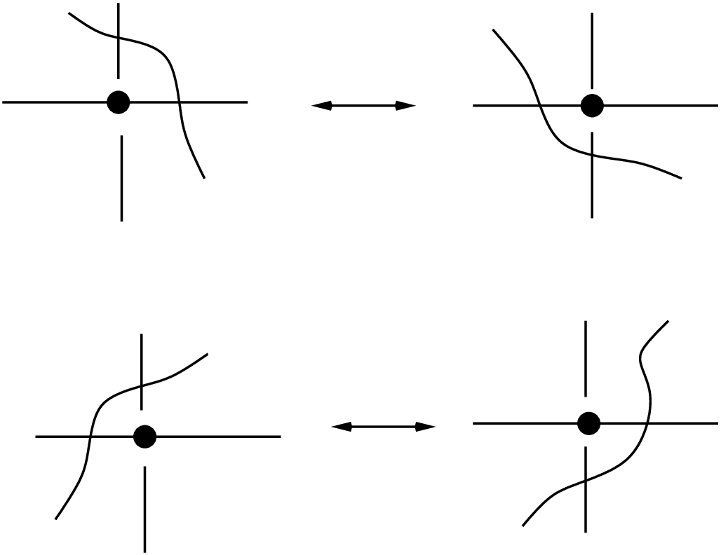
- •
Plane isotopy.
- •
Switching the over/under arcs at an accidental crossing.
- •
The -graph versions of oriented Reidemeister moves, called R-moves (i.e. formally the usual ones if only accidental crossings are involved, or the Reidemeister move of type III shown in Figure 10 (the orientation being understood) when a dotted crossing is involved).
6.2. Changing the weak branching
Given a -graph representing a weakly branched triangulation , and an arbitrary change of weak branching , we want to describe a systematic way to modify to a -graph representing . We begin with the local changes of branching on a given tetrahedron.
6.2.1. The action
Consider a branched tetrahedron with -ordered vertices and -facets , as usual. Let be the symmetric group on the set . There is a natural correspondence between the elements and the branchings on such that . The branching induces a branching on each facet , that is a labelling of the vertices of by elements of . For every , also the branching induces a branching on (note that these facets are still ordered with respect to , not ), and the transition from to is encoded by a permutation . Clearly we have:
Lemma 6.1.
(1) The branching signs and coincide if and only if .
(2) The -facet has the same - and -transverse co-orientations if and only if .
Let denote a dotted -graph crossing that encodes as in Figure 4. We call a -tangle; we consider it as a planar tangle properly embedded in a -disk , with endpoints on labelled by . One can assume that the crossing is central to , and that the arcs joining it to the endpoints are contained in two oriented diameters of . We want to describe an algorithm that produces, for every , a new decorated -tangle in , with the same unoriented arc-germs as at . Hence the arcs of and will be in natural correspondence and oriented by and respectively. The tangle will verify the following properties:
- •
contains one dotted crossing. According to the last Lemma, if and only if . Hence, given , we know the sign .
- •
can replace in every -graph obtained after a change of weak branching acting as on the corresponding branched tetrahedron of .
- •
Each of the four arc-germs of at is labelled by an element of , which will eventually contribute to the edge coloring of .
An auxiliary construction. Consider the two basic tangles in a -disk , made by two oriented simple arcs , that either are disjoint or intersect transversely at one point, without any over/under information at the crossing point. A -labelling of the free endpoints of is admissible if it respects the following conditions:
(a) The endpoints labelled by (resp. ) belong to different arcs and are both either the initial or the final endpoint of the corresponding arc.
(b) (resp. ) label the endpoints of the same arc.
These conditions are satisfied by the labels of the tangles of Figure 4; recall that in this figure, (resp. ) if and only if label initial (resp. final) endpoints. By the same rule we give every basic tangle an admissible -labelling, denoted by , and a sign . Note also that in Figure 4, the arc with endpoints labelled by passes over the other arc. Now we convert into a -tangle as follows:


(c) If , perform an oriented Reidemeister move of type II of the arc with labels over the other arc, thus creating two crossings. Only one of them can be made into a dotted crossing so that its sign agrees with (see some examples in Figure 11).
(d) If and cross at one point, let be the arc with labels, and a small open interval in the interior of the arc with labels, such that contains the crossing point. Let pass over , put a dot at the crossing point, and turn so that the crossing sign and agree. Finally complete to an -tangle with the same endpoints as , by introducing or accidental crossings on opposite sides of with respect to (see some examples in Figure 12).
The algorithm :
- (1)
Remove the interior of a smaller concentric sub-disk of . Each endpoint of , say , , is connected by an oriented sub-arc to a point on .
- (2)
There is only one basic tangle in such that the -labelling of the endpoints is admissible and . As in the auxiliary construction, convert into an -tangle in ; glue it to the four sub-arcs , and denote by the resulting -tangle in .
- (3)
The -tangle is obtained from by giving a label to each sub-arc as follows. Recall the permutation defined before Lemma 6.1; the - and -orientations of coincide one to each other iff ). Then set:
- •
, if the -orientation of coincides with the orientation pointing towards the center of ;
- •
otherwise.
- •
6.2.2. Iterations
Assume that , where by definition . Then we can produce by iterating two times the preceding algorithm. We get a sequence of nested disks
a subdivision of the segment into sub-arcs
and a factorization of the permutation associated to :
The “adjacent” transpositions form a standard set of generators of . Let where each is such a generator. Then we can produce again by iterating times the algorithm. We get a sequence of nested disks
a subdivision of the arc of into sub-arcs
and a factorization of the permutation associated to the arc :
Lemma 6.2.
Every transposition belongs to the set .
Proof. It is enough to check the case (see Figure 13).
For future application, it is convenient to associate a symbol to each sub-arc of , that indicates its label and depends on its -orientation:
- •
If the -orientation is outgoing (i.e. opposite to the one pointing towards the center of ), then let this symbol be , or (a “source”) if is a transposition;
- •
if the -orientation is ingoing, then let this symbol be , or (a “pit”) if is a transposition.
Under concatenation of sub-arcs, adjacent symbols are separated by or . Here are examples:
Letting , in the case of we get:
- •
or if and induce on the same orientation;
- •
or otherwise.
We can also make simplifications of the form:
and so on, so that the concatenation of symbols of sub-arcs eventually reduces to , , or alternating pits and sources carrying the transpositions and . In Figure 13 we show graphically the result when and varies in ; we dropped the notation for the symbol . The case is similar.

6.2.3. Oriented -moves
We call a -move. If and define the same pre-branching then we say that it is an oriented -move. Set
generates a subgroup of isomorphic to via the map .
Lemma 6.3.
For both , induces an oriented -move iff .
Proof. Looking at Figure 2 anti-clockwise from the top left, and denoting by the first branching (so that ), the others are successively , , , . Hence . One can do similarly when .
Figure 14 shows the oriented -moves for and for .

6.2.4. Globalization
Let be an -graph encoding , and another weak branching on . We want to produce an -graph encoding . For every abstract branched tetrahedron of there is a permutation such that the restriction of the transit to is . Applying at every crossing of the algorithm , we get a diagram . Forgetting the orientations, there is a natural correspondence between the edges of and . Let be an edge of with color . Denote by the corresponding edge of . According to the last step of the algorithm, is labelled by “initial” and “final” permutations . There is an alternative:
- •
Both and belong to (in such a case and have compatible orientations); then the color is defined by
- •
Both and do not belong to (in such a case and have opposite orientations); then the color is defined by
The oriented -moves have the nice feature to be local and independent one to each other. On the contrary, a family of permutations as above must satisfy non trivial global constraints to induce a change of weak branching . Fortunately, the following local/global calculus on -graphs (introduced in [9]) covers the general case.
Lemma 6.4.
Any change of -graphs corresponding to a change of weak branching is a composition of a finite sequence of moves of the following types:
- (1)
The moves of Subsection 6.1;
- (2)
The oriented -moves;
- (3)
(A non-local “circuit” move). Let be a simple circuit of , ie. a circuit with one component. Assume that each edge of is the upper strand at each crossing through which passes. Then is obtained by acting on each of these crossings with the transposition . Equivalently, is obtained by reversing the orientation of and keeping the -color unchanged at every edge of .
Proof. The equivalence between the two descriptions of the non-local “circuit” move is clear. Let be as in the statement. The set of edges of where the pre-branchings associated to and disagree is the union of non-overlapping simple circuits , oriented by . Using oriented -moves one can modify so that eventually passes over at each crossing where it goes through. Then change its orientation. Doing similarly with , , one ends up with .
6.3. Transits
It is well-known that two “naked” triangulations and of can be connected by a finite sequence of -dimensional Pachner’s moves, also called MP and bubble moves. The MP moves, also called “” moves, are illustrated in Figure 15 in terms of triangulations and dual spines. Branched versions of the bubble moves are shown in Figure 16 in terms of -graphs.

Definition 6.5.
Let and be pre-branched triangulations of . A move (either bubble or MP, positive or negative) lifts to a pre-branching transit if and only if and coincide on every common -face of and . We say that lifts to a -transit of weakly-branched triangulations if it induces a pre-branching transit . If and are branched triangulations, then is a -transit if and coincide on every common edge of and .
Figure 16 shows the different bubble -transits in terms of normal -graphs (recall Remark 2.11), and the decorations , of the dual square edges according to Figure 8. Figure 17 and 18 show an example of MP -transit in terms of branched triangulations and normal -graphs; note that for all -simplices (resp. dotted crossings). It is called the Schaeffer -transit, and plays a distinguished role in the study of matrix dilogarithms (see Section 8).


The following Lemma will be useful in applications to the QH state sums. Denote by the equivalence relation on the set of weakly branched triangulations, defined by -transits .
Lemma 6.6.
The equivalence relation is generated by the following two transformations:
- •
Change the weak-branching by moves preserving the pre-branching (ie. dually do oriented -moves, see Lemma 6.4).
- •
Perform -transits which look like -transits at the sub-patterns of tetrahedra involved in the move.

Proof. The proof for bubble moves is easy and basically illustrated in Figure 16 in terms of -graphs. Consider a positive MP -transit , and the two tetrahedra of modified by the transit. At their common -face one of the following possibilities is realized:
(1) there are exactly two square edges which are both not monochromatic (i.e. each one inherits different , labels from the pre-branchings of the two tetrahedra);
(2) there is exactly one square edge which is monochromatic (either or ), and the other two edges are monochromatic (either or coupled with the empty label).
Moreover, this information at determines completely the co-orientations of the three -faces produced by the transit, and hence determines the pre-branching transit . Then, it is enough to realize the above possibilities by means of -transits (changing the weak branchings before and/or after the transit, if necessary, by moves preserving the pre-branching). Figure 19 shows it in terms of (decoded) normal -graphs. Clearly this realization is not unique.
7. State sum invariance over weakly branched triangulations
Let be a weakly branched QH triangulation of a pattern ; and verify the defining equations of the spaces in Definition 3.7, and those of Definition 4.7 (resp. 5.1) if is a pattern over a cusped manifold (resp. a QHFT pattern).
We want to prove that is an invariant of . In the case when is a branched triangulation we achieved this result in [3, 4, 5] by introducing the notion of QH transit . A QH transit is such that: is a -transit, the tuples and coincide on the “common” tetrahedra of and , and for every common edge we have (see Section 3.2 for the notations, where is , and so on)
| (60) |
QH triangulations related by QH transits encode a same pattern . Moreover:
- •
is invariant under any QH transit.
- •
Any two branched QH triangulations of are related by a finite sequence of QH transits and branching changes.
- •
is invariant under any change of the branching .
Clearly these three facts prove the invariance of . We follow the same strategy when is an arbitrary weak branching. Since the QH transits are local transformations, we define QH transits by requiring that the -transit restricts to a genuine -transit on the tetrahedra modified by the move. Then, trivially is again invariant under QH transits, and using Lemma 6.6 and the results of [3, 4, 5] it is easy to see that any two weakly branched QH triangulations of are related by a finite sequence of QH transits and changes of weak branching. So it remains to show:
Proposition 7.1.
For any change of weak branching we have
In order to develop the proof we need to fix some conventions regarding the contraction of tensors, and to describe the relations between tetrahedral tensors related by a change of branching. This is the content of the two following subsections.
7.1. Formal conversion of tensor networks
Recall the notation . We use the canonical isomorphism sending the standard basis to the dual basis. Let be associated to a -tangle as in Figure 9, according to the conventions of Section 3.1. Let . Assuming that , under the natural isomorphisms
| (61) |
we see that belongs to , where as usual is the copy of associated to the -th face of . Consider if , and if , where is the copy of associated to the th-face according to . By using or the canonical isomorphisms , we get further canonical isomorphisms
Denote by the operator supported by , defined as the image of via such an isomorphism. We call the formal -conversion of . There are explicit identities between the matrix elements of and . Following our conventions for the index positions, we get for example
Let be a QH tensor network supported by a weakly branched triangulation . For any change of weak branching , the formal conversions of the tetrahedral tensors of match to produce a new tensor network , supported by . The state sums associated to and being total contractions, it is tautologically evident that they take the same values.


The formal conversion of tensors can be widely applied. Here is a second example that we use below. Let be any matrix. We interpret as an endomorphism of . There are two formal conversions of , and , which are bilinear forms on and on respectively, defined by:
| (62) |
Note that we have also , where is the transpose matrix of , that is, the adjoint endomorphism. Figure 20 shows a graphical encoding of these identities. If is symmetric, the position of the indices is immaterial. Such formal conversions satisfy a few relations shown in Figure 21, where , and denote matrices and we assume that . Note that in every case the index is traced out, and the top/right picture represents the matrix element of a composite endomorphism
7.2. The relations between and
Consider a change of branching , . It is enough to treat the case where is one of the standard generators . Consider the algorithm of Section 6.2. Associate a tensor network to as follows:
- •
Associate to the dotted crossing of .
- •
Using the matrices and of Section 3.2, replace with , with , with , with , and with .
Contracting the tensor network we get a tensor which has the same type as , since both have the same oriented arc-germs at . The next Proposition rephrases the content of Lemma 3.3 of [3] and Corollary 5.6 of [4]. Matrix indices are raised or lowered using the standard inner product of (see Section 7.1).
Proposition 7.2.
If , then
More precisely, exchanging the roles of and and setting , we have:
The main properties of and are described in the following Lemma.
Lemma 7.3.
We have:
- (1)
.
- (2)
where is given by
- (3)
.
Proof. (1) is immediate. We have . For all non vanishing coprime integers , with set
The sum in has this form for , . By [28, page 86-87] we have
where if mod, and if mod. Hence , and (2) follows easily from this. As , it is enough to prove the last statement for . This follows: ; ; finally .
7.3. Proof of Proposition 7.1.
By Lemma 6.4 we can assume that corresponds to an oriented -move or a circuit move on the associated -graphs. A circuit move preserves the -color of every edge , and produces one extremal pit and one extremal source associated to the matrices and at the endpoints of each edge of the circuit. Hence is preserved, as it is the contraction of a tensor network. Consider the generating oriented -move associated to , and the tensor resulting from the formal conversion of the sequence
as before Proposition 7.2. From Figure 14 we see that an edge of carries the matrix if ( being the arc of associated to ), and that carries if . Otherwise it carries the identity matrix. By the relation proved in Lemma 7.3, the sum in is changed by a factor when and , or when and . The term of compensates exactly such factors.
8. Resolution of the sign anomaly
In this Section we prove Theorem 1.1 (3) and the analogous result for QHFT partition functions:
Proposition 8.1.
Let be a QHFT pattern or a pattern over a cusped manifold. If , or and the bulk -weight of vanishes, then is defined up to multiplication by -th roots of unity.
Proof. We combine several results described below in Sections 8.1 and 8.2. By Corollary 8.6, for any odd the invariance of under QH transits holds true up to multiplication by -th roots of unity. If , we have , so has no sign anomaly with respect to any change of weak branching (Proposition 7.2). If and , the same is true by Lemma 8.7 and 8.8. Then the conclusion follows as explained before Proposition 7.1
Let be a pattern for which can be defined by using branched triangulations, as in [3, 4, 5]. Then or , so we can wonder if the sign anomalies occuring in Proposition 7.2 disappear because of global compensations. This is eventually true.
Proposition 8.2.
For any pattern as above, is defined up to multiplication by a -th root of unity, with no assumption on the weights of .
Proof. By a result of Costantino [13], any change of branching can be achieved by means of a finite sequence of branching transits. The conclusion follows from Corollary 8.6.
Remark 8.3.
One can ask if a weakly branched version of Costantino’s result holds true: given weakly branched triangulations and of that differ only by the weak branchings, are they related by a sequence of oriented -moves and “local” -transits ? The answer is negative. In fact, we know that the state sums have no sign anomaly with respect to QH transits and oriented -moves, but there are examples of weakly branched triangulations admitting circuit moves along circuits such that .
8.1. Behaviour of the sign anomaly under QH transits
Recall the formula (19). The matrix dilogarithms satisfy Proposition 7.2, whereas the basic dilogarithms satisfy the relations ([4], Proposition 5.3):
| (63) |
Define the transits of -th root cross ratio moduli like in (60), by replacing with the total -th root modulus at all edges of and . Clearly any QH transit induces a transit of -th root cross ratio moduli.
Theorem 8.4.
([4], Theorem 5.2) The basic matrix dilogarithm identity supported by the Schaeffer transit of -th root cross ratio moduli holds true up to an -th root of unity anomaly.
The proof goes as follows. The basic matrix dilogarithm identity supported by the Schaeffer QH transit is equivalent to the following equality in :
| (64) |
where and are explicit matrices satisfying , , and , being a primitive -th root of , and for a tensor satisfying (on the appropriate space: , , etc.) one sets
| (65) |
In (64), means acting on the second and third tensorands, i.e. , etc. One can check that is uniquely determined up to multiplication by scalars by the functional relation
| (66) |
The identity (64) lifts to the algebra generated by and , so we have to show
| (67) |
when , , and . To do it, one uses crucially the relations between -th root cross-ratio moduli implied by the Schaeffer QH transit. One shows that commutes with ; hence is a function of . Moreover, it satisfies
| (68) |
Comparing with (66) we see that and are equal up to a multiplicative constant . We introduce an -th root of the reciprocal of in each entry of so that (this is the term in (18)). Then and . As a result the tensor can be expressed in terms of for a suitable (see [4], formulas (32) and (33)).
The basic matrix dilogarithm identities hold true up to an -th root of unity anomaly only for some branching transits. From (63) one deduces the following table of the anomalies produced by the symmetries of the Schaeffer transit (it is enough to consider those induced by the transpositions on the vertex ordering used in Figure 17). The transits of -th root moduli imply that the anomalies are equal for the symmetries induced by and , but differ for and because of the occurence of the opposite exponents , for the -th root moduli , respectively. For instance , but we see .
|
|
Replacing the tensors with we have:
Proposition 8.5.
The matrix dilogarithm identities hold true up to an -th root of unity anomaly for all QH transits.
Proof. Since we have the identity (64), in the case of the Schaeffer QH transit identity it is enough to compare the symmetrization factors at both sides. They are ():
and
A computation shows that the transits of log-branches and charges imply that the two exponentials are equal, and with the flattening transit mod that the signs are equal. To prove the claim for all others QH transits we compare the anomalies resulting from symmetries on the Schaeffer QH transit. Since all QH transits are branched, the actions by the matrices , due to Proposition 7.2 cancel out along interior faces. The following table shows the sign anomalies. Again, the transit of charges implies that they are equal at both sides.
|
|
As usual, the identities for the bubble moves are formal consequence of those for the moves. This concludes the proof.
Corollary 8.6.
Let be any QH transit of weakly branched QH triangulations of a pattern . Then
Proof. If the transit is supported by a MP move it is immediate that , hence the conclusion follows from Corollary 8.5. If it is supported by a positive bubble move, spelling the contribution of each term we realize that if
then
and . Hence , as it must be in order to ensure the invariance under the bubble move, which increases by the number of internal vertices.
8.2. Behaviour of the sign anomaly under a change of weak branching
A change of weak branching modifies by its sub-factors and
By the proof of Proposition 7.1, and the unnormalized QH state sum have reciprocal variations. So it remains to analyze the behaviour of with respect to oriented -moves and the circuit move of Lemma 6.4.
It is relevant here to clarify the nature of . By extending Chapter 7 of [7], the paper [9] provides a combinatorial realization of spin structures on -manifolds, based on weakly branched triangulations instead of branched ones. In particular, one associates to every weakly branched triangulation a framing of the manifold defined along , and computes a cellular cochain representing the obstruction to extend over the whole of the spine . Consider the cellular -chain , where varies among the -regions of . It is a fact that
How , whence , varies with the weak branching is part of the theory developed in [9]. As a consequence we get:
Lemma 8.7.
For any change of weak branching preserving the induced pre-branching we have
Proof. It is enough to show the result for one generating oriented -move . By local inspection one checks that , so . On the other hand, using Proposition 7.2, the factorization , and the relation , we see that changes the unnormalized QH state sum by . Hence the two sign variations are equal.
Lemma 8.8.
For any change of weak branching induced by one circuit move along a circuit we have
where is the bulk -weight of . In particular, has no sign anomaly if .
Proof. Let us realize the circuit move in terms of -graphs. By the third identity of Proposition 7.2 the move changes the state sum by one factor for each crossing of . It is easy to check that their product computes . On the other hand , so that .
9. Examples
In this section we describe the quantum hyperbolic invariants of the figure-eight knot complement, its “sister”, and the complement of the knot .
We give also some samples of numerical computations obtained by using Maple, which are part of our current analytical and numerical exploration of the QHI. At first we quote that they corroborate the invariance of the QH state sums with respect to the choice of flattenings or charges having the same weights. In the case of the sister manifold, they confirm also the invariance of the QH state sums supported by weakly branched triangulations. Moreover, the numerical computations that we present below are proving:
- •
The actual dependence of the invariants on the weights (and not only on the characters ).
- •
This dependence persists as .
- •
For some weights the invariants seem to grow exponentially with , and yield instances of the volume conjecture, and for some other weights they do not.
Other interesting phenomena happen, that deserve to be understood. For instance, in the case of the complements of the knots and , it appears that the asymptotical behaviour of the absolute values of the invariants do not depend on the values on the meridian of the charge weights or the flattening weights.
9.1. Notations
Let be a quantum -simplex. Put , . We call an edge color. In order to simplify the formulas we denote the -th roots of the cross-ratios by bold letters (rather than , as we did in (14)), and call them q-shape parameters. So
For any cusped manifold and any QH triangulation of , we have the tetrahedral and edge relations (see (15), (22) and (25))
and
where, as usual, and if is the edge or the opposite edge of a quantum -simplex of , and . We denote by the variety thus defined by the q-shape parameters, and call it the QH gluing variety (NB: it coincides with the variety of Section 3.2; to simplify notations, here we drop the reference to the charge ).
As usual, denote by a compact -manifold with one torus boundary component such that is diffeomorphic to the interior of . We compute the invariant by means of the function on introduced after Definition 3.5. As is formulated in terms of q-shape parameters and charges, we express equivalently as , using the classes and obtained from the flattening weights and by replacing the flattenings by the edge colors in the respective formulas (see Definition 4.10, and (26) for ). Clearly and . We call and the reduced boundary and bulk weights. By (1) and (28) one has the compatibility relations
| (69) |
for all .
We consider triangulations with ordered tetrahedra. We denote by (resp. , resp. , resp. ) the triples of cross-ratios (resp. q-shape parameters, resp. edge colors, resp. charges) of the tetrahedra, in the same order.
9.2. The figure-eight knot complement
The Epstein-Penner decomposition of is an ideal triangulation having a branching and two tetrahedra, with opposite -orientations. We showed the dual spine in Figure 6. We denote by the tetrahedron with positive -orientation. In [5] we described the flattenings at positive points of the gluing variety , as well as the charges and the QH state sums carried by .
9.2.1. The QH gluing variety
The gluing variety is the irreducible plane curve with coordinates and defining equation , which may be written as (as usual and similarly for the ’s). The point realizes the complete hyperbolic structure. Let and be the canonical longitude and the meridian of the figure-eight knot, and let . The dilation factors of the holonomy are given by
The tetrahedral and edge relations between q-shape parameters are
Together with the identities and , these relations define . Using the tetrahedral relations it is easy to see that the two edge relations are equivalent. Recall the reduced weights and introduced in Section 9.1. By (69) we have
| (70) |
As is a knot complement, the bulk weight is determined by , and similarly is determined by . Moreover, , so is non zero if and only if mod.
Over the point we have and , and the tetrahedral relations, the edge relations, and the compatibility relations with imply the following expressions of the edge colors and in terms of and : , , and
| (71) |
For points lying over a sufficiently small neighborhood of the point , the same expressions are valid if one replaces with .
Similarly the charges and are given by
| (72) |
Let be a closed hyperbolic -Dehn filling of represented by in a small neighborhood of . The holonomy factors through the quotient map to define the holonomy of . One has
| (73) |
and letting , be such that , the reduced weight satisfies if and only if
| (74) |
Similar formulas express the identity .
9.2.2. The state sum formulas
Recall the notations of Section 3.1.2. For any and any charge on , the QH state sum
| (75) |
computes the invariant , and defines a (non-constant) rational function on . By a surgery theorem proved in [5], at points where and satisfy as above, coincides with the -th quantum hyperbolic invariant of the closed manifold , where is the surgery core.
9.2.3. Some numerical results
Denote by the holonomy of given by the shape parameter and the solution of the gluing equation such that has positive imaginary part and has negative imaginary part. So is the hyperbolic holonomy.
Recall that and are determined by and respectively. In the following table we present some values of up to 4 digits, where and are as indicated on the top and the left of the corresponding column and row ( defines the holonomy of the -Dehn filling of ), and we put and , where has the collection of shape parameters determined by , and a (compatible) flattening such that at the complete hyperbolic structure.
|
|
Note that the table shows that the invariants depend on the character and the weights. Also, the first two columns show a symmetry about (that is, when , about ), corresponding to a change of orientation of . The dominant rows are for or (that is, when , about or ).
Now consider the behaviour of as . Put , where the arguments are as above except that we fix (the complete hyperbolic structure). Let be divided by , the product of the matrix dilogarithm symmetrization factors. Note that and are equivalent as . The following table gives a sample of values of , where takes the values indicated in the first row.
|
|
Note that the dependence on the weights persists as . Further numerical computations show that converges to as .
9.3. The complement of the knot
The ideal triangulation of with smallest complexity has three tetrahedra , , , and it has a branching that gives each tetrahedron the negative branching orientation. This triangulation is the one provided by Snappea; we keep the same ordering of tetrahedra. The branching is determined by the ordering it induces on the set of vertices of , which is obtained from that provided by Snappea by applying the permutation .
9.3.1. The QH gluing variety
The edge relations of are , , and . By the tetrahedral relations they reduce to two independent relations, so the gluing variety of is the irreducible curve in with coordinates and defining equations
The complete hyperbolic structure is realized by the point given up to digits by (the imaginary parts are negative since all tetrahedra have the negative branching orientation)
Since is irreducible and is a positive point, it is a rich variety. Let and be the canonical longitude and the meridian of the knot, and let . The dilation factors of the holonomy are given by
The tetrahedral and edges relations between q-shape parameters are (note that the exponents on the left of the edge relations are due to the negative branching orientation of the tetrahedra)
Together with the identity and the similar ones for the ’s and the ’s, these relations define . Using the tetrahedral relations it is easy to see that any of the edge relations is a consequence of the other two. By definition, the weights satisfy
As is a knot complement, the bulk weight is determined by , and similarly is determined by . Moreover , so is non zero if and only if mod.
At the complete hyperbolic structure we have and , and the tetrahedral relations, the edge relations, and the compatibility relations with imply the following expressions of the edge colors , and , in terms of , and : , , , and
If lies over a point in a small neighborhood of , then the same expressions are valid if one replaces with .
Similarly, the charges , and are given by
9.3.2. The state sum formulas
For any and any charge on we have (here we denote by the tensor
The QH state sum computes the invariant and defines a (non-constant) rational function on . As for the figure-eight knot complement, and using the same notations, at a point such that , coincides with the -th quantum hyperbolic invariant of the triple obtained by hyperbolic -Dehn filling of .
9.3.3. Some numerical results
Keeping the same notations as in Section 9.2.3, we present below some values of up to 4 digits, and some values of . For each of the shape parameter that we consider, with the exception of , there are two distinct points such that both , and have negative imaginary parts. We take take again , but now and hence , where is determined by , and is a (compatible) flattening such that, at the complete hyperbolic structure, takes the value indicated on the left of each row.
|
|
|
|
Further numerical computations show that converges as to .
9.4. The sister of the figure-eight knot complement
( in Snappea’s census). This cusped manifold is obtained by Dehn surgery on a component of the Whitehead link (see [39], [31]). The figure eight knot complement and its sister have the smallest volume of any orientable, cusped hyperbolic -manifold. Hyperbolic Dehn surgery on induced by and Dehn surgeries on the Whitehead link yields the Fomenko-Matveev-Weeks manifold, which has the smallest volume of any closed orientable hyperbolic 3-manifold (approximately 0.9427…) [21].
The Epstein-Penner decomposition of is the ideal triangulation with two tetrahedra considered in Example 2.12 and 4.11. We have already described a weak branching on where both tetrahedra have positive branching orientations, and computed the charges, the flattenings at positive points of the gluing variety , and the QH state sums carried by .
9.4.1. The QH gluing variety
The edge relations of are and . By the tetrahedral relations they are equivalent, so the gluing variety is the irreducible plane curve with coordinates and defining equation . The point realizes the complete hyperbolic structure (thus and are regular ideal tetrahedra, as in the case of the figure-eight knot complement). There is a basis of where the dilation factors of the holonomy are given by
| (76) |
The tetrahedral and edges relations between q-shape parameters are
Together with the identity and the similar one for the ’s, these relations define . Using the tetrahedral relations it is easy to see that the two edge relations are equivalent. The reduced weights satisfy the compatibility relations
Here we note that , and that the curve or generates . So the bulk weight is determined by , and similarly is determined by . Moreover mod, so is non zero if and only if mod.
At the complete hyperbolic structure we see that and , and the tetrahedral relations, the edge relations, and the compatibility relations with imply the following expressions of the edge colors and in terms of and :
| (77) |
For points lying over a small neighborhood of , the same expressions are valid if one replaces with .
9.4.2. The state sum formulas
For any and any charge on we have (again we denote by the tensor )
The QH state sum computes the invariant and defines a (non-constant) rational function on . As for the previous examples, at a point such that , coincides with the -th quantum hyperbolic invariant of the triple obtained by hyperbolic -Dehn filling of .
9.4.3. Some numerical results
We keep the same notations as in Section 9.2.3 and we take again , but now both and have positive imaginary part, and the value of is given by (on the left of each row), , and a flattening such that . The following table presents values of up to 4 digits.
|
|
References
- [1] H. Bai, Quantum Teichmüller spaces and Kashaev’s -symbols, Alg. Geom. Topol. 7 (2007) 1541–1560
- [2] H. Bai, F. Bonahon, X. Liu, Local representations of the quantum Teichmuller space, arXiv:math.GT/0707.2151
- [3] S. Baseilhac, R. Benedetti, Quantum hyperbolic invariants of 3-manifolds with -characters, Topology 43 (6) (2004) 1373–1423
- [4] S. Baseilhac, R. Benedetti, Classical and quantum dilogarithmic invariants of flat -bundles over -manifolds, Geom. Topol. 9 (2005) 493–570
- [5] S. Baseilhac, R. Benedetti, Quantum hyperbolic geometry, Alg. Geom. Topol. 7 (2007) 845–917
- [6] S. Baseilhac, R. Benedetti, The Kashaev and quantum hyperbolic invariants of links, J. Gökova Geom. Topol. 5 (2011) 31–85
- [7] R. Benedetti, C. Petronio, Branched Standard Spines of -manifolds, Lecture Notes in Mathematics 1653, Springer (1997)
- [8] R. Benedetti, C. Petronio, Lectures on Hyperbolic Geometry, Universitext, Springer Verlag (1992)
- [9] R. Benedetti, C. Petronio, Spin structures on -manifolds via arbitrary triangulations, to appear in Algebraic and Geometric Topology
- [10] D.W. Boyd, F. Rodriguez-Villegas, Mahler’s measure and the dilogarithm (II), with an appendix by N.M. Dunfield, arXiv:math.NT/0308041
- [11] S. Boyer, X. Zhang, On Culler–Shalen seminorms and Dehn filling, Ann. of Math. (2) 148 (3) (1998) 737–801
- [12] D. Bullock, Rings of -characters and the Kauffman bracket skein module, Comment. Math. Helv. 72 (4) (1997) 521–542
- [13] F. Costantino, A calculus for branched spines of 3-manifolds, Math. Zeitschrift 251 (2) (2005) 427–442
- [14] D. Cooper, M. Culler, H. Gillet, D.D. Long, P.B. Shalen, Plane curves associated to character varieties of -manifolds, Invent. Math. 118 (1994) 47–84
- [15] Y.-E. Choi, Positively oriented ideal triangulations on hyperbolic -manifolds, Topology 43 (2004) 1345–1371
- [16] A. Champanerkar, A-polynomial and Bloch invariants of hyperbolic -manifolds, PhD Thesis, Columbia University (2003)
- [17] M. Culler, P.B. Shalen, Varieties of group representations and splittings of –manifolds, Ann. of Math (2) 117 (1) (1983) 109–146
- [18] N. Dunfield, Cyclic surgery, degree of maps of character curves, and volume rigidity for hyperbolic manifolds, Invent. Math. 136 (1999) 623–657
- [19] S. Freed, Classical Chern-Simons Theory, 1, Adv. in Math. 113 (1995) 237–303
- [20] S. Francaviglia, Hyperbolic volume of representations of fundamental groups of cusped -manifolds, Internat. Math. Res. Not. 9 (2004), 425–459
- [21] D. Gabai, R. Meyerhoff, P. Milley, Minimum volume cusped hyperbolic three-manifolds, Journal Amer. Math. Soc. 22 (4) (2009) 1157–1215
- [22] A. Hatcher, Algebraic Topology, Cambridge Univ. Press (2002)
- [23] M. Kapovich, Hyperbolic Manifolds and Discrete Groups, Birkahäuser, Prog. Math. 183 (2010)
- [24] R.M. Kashaev, Quantum dilogarithm as a 6j-symbol, Mod. Phys. Lett. A Vol. 9 (40) (1994) 3757–3768
- [25] R.M. Kashaev, A link invariant from quantum dilogarithm, Mod. Phys. Lett. A Vol. 10 (40) (1995) 1409–1418
- [26] R. M. Kashaev, The hyperbolic volume of knots from the quantum dilogarithm, Lett. Math. Phys. 39 (1997) 269–275
- [27] P. Kirk, E. Klassen, Chern-Simons invariants of -manifolds decomposed along tori and the circle bundle over the representation space of , Comm. Math. Phys. 153 (3) (1993) 521–557
- [28] S. Lang, Algebraic Number Theory, Springer (1994)
- [29] F. Luo, S. Schleimer, S. Tillmann Geodesic ideal triangulations exist virtually, Proc. Amer. Math. Soc. 136 (2008) 2625–2630
- [30] F. Luo, S. Tillmann, T. Yang Thurston’s spinning construction and solutions to the hyperbolic gluing equations for closed hyperbolic 3-manifolds, Proc. Amer. Math. Soc. 141 (1) (2013) 335–350.
- [31] S.V. Matveev, A.T. Fomenko, Constant energy surfaces of Hamiltonian systems, enumeration of three-dimensional manifolds in increasing order of complexity, and computation of volumes of closed hyperbolic manifolds, Russian Math. Surveys 43:1 (1988) 3–24
- [32] H. Murakami, J. Murakami, The colored Jones Pulynomials and the simplicial volume of a knot, Acta Math. 186 (2001), 85-104
- [33] W. D. Neumann, Combinatorics of triangulations and the Chern-Simons invariant for hyperbolic -manifolds, Topology’90 (Columbus, OH, 1990), De Gruyter, Berlin (1992) 243–271
- [34] W.D. Neumann, Extended Bloch group and the Cheeger-Chern-Simons class, Geom. Topol. 8 (2004) 413–474
- [35] W.D. Neumann, D. Zagier, Volumes of hyperbolic 3-manifolds, Topology 24, 307–332 (1985)
- [36] C. Petronio, J. Porti, Negatively oriented ideal triangulations and a proof of Thurston’s hyperbolic Dehn filling theorem, Exp. Math. 18 (2000) 1–35
- [37] P.B. Shalen, Representations of –manifold groups, Handbook of geometric topology, North–Holland, Amsterdam (2002) 955–1044
- [38] W.P. Thurston, The geometry and topology of -manifolds, Princeton Univ. Press (1979)
- [39] J. Weeks, Hyperbolic structures on 3-manifolds, Ph.D. thesis, Princeton Univ. (1985)
- [40] T. Yoshida, The -invariant of hyperbolic -manifolds, Invent. Math 81 (1985) 473–514