Compositional Verification of Evolving Software Product Lines
Abstract
This paper presents a novel approach to the design verification of Software Product Lines(SPL). The proposed approach assumes that the requirements and designs are modeled as finite state machines with variability information. The variability information at the requirement and design levels are expressed differently and at different levels of abstraction. Also the proposed approach supports verification of SPL in which new features and variability may be added incrementally. Given the design and requirements of an SPL, the proposed design verification method ensures that every product at the design level behaviorally conforms to a product at the requirement level. The conformance procedure is compositional in the sense that the verification of an entire SPL consisting of multiple features is reduced to the verification of the individual features. The method has been implemented and demonstrated in a prototype tool SPLEnD (SPL Engine for Design Verification) on a couple of fairly large case studies.
1 Introduction
Large industrial software systems are often developed as Software Product Line (SPL) with a common core set of features which are developed once and reused across all the products. The products in an SPL differ on a small set of features which are specified using variation points. The focus of this paper is on modeling and analysis of SPLs which have drawn the attention of researchers recently [1, 2, 3].
Many approaches have been proposed to describe SPLs, the most prominent one being feature diagrams. All these proposals seem to assume a global view of SPL as they start with a complete list of features and the variation points using a single vocabulary. All the subsequent SPL assets, like requirement documents, design models, source codes, test cases, documentations, share the same definition and vocabulary [4, 5]. The assumption of a single homogeneous and global view of variability description is inapplicable in many practical settings, where there is no top level complete description of features and variabilities. They often evolve during the long lifetime of an SPL as new features and variabilities are added during the evolution. Further, SPL developers tend to use different representations and vocabulary of variability at different stages of development: at the requirement level, a more abstract and intuitive description of variation points are used, while at the design level, the efficiency of implementation of variation points is of primary concern. For example, consider the case of an automotive SPL, where one variation point is the region of sale (eg. Asia Pacific, Europe, North America etc). At the requirement level, this variation point is expressed directly as an enumeration variable assuming one value for every region. Whereas, at the design level, the variation point is expressed using two or three boolean variables; by setting the values of the boolean variable appropriately, the behavior specific to a region is selected at the time of deployment.
We present a design verification approach that is more suited to the above kind of evolving SPLs in which different representation of variabilities would be used at the requirement and design level. One natural and unique problem that arises in this context is to relate formally the variation points expressed at different levels of abstractions. Another challenge is the analysis complexity: the number of products is exponential in the number of variation points and hence product centric analyses are not scalable. We propose a compositional approach in which every feature of the SPL is first analyzed independently; the per-feature analysis results are then combined to get the analysis result for the whole SPL.
For capturing variability in the behavior of an SPL, we have extended the standard finite state machine model, which we call Finite State Machines with Variability, in short, FSMv. The behavior and variability of a feature at the requirement and design level can be modeled using FSMv. We define a conformance relation between FSMvs to relate the requirement and design models. This relation is based upon the standard language containment of state machines.
One unique feature of FSMv is that it provides a compositional operator for composing the feature state machines to obtain a model for an SPL. This operator thus enables incremental addition of features and variabilities. The proposed verification approach exploits the compositional structure of the SPL models to contain the analysis complexity.

Figure 1 summarizes the proposed approach. It shows an SPL composed of features to . Each feature has an FSMv model of its requirements (called FSMr) and an FSMv model derived from its design (called FSMd). The proposed analysis method checks whether the FSMd of every feature conforms to its FSMr ( check). The output of this first step is a conformance relation between each pair of FSMr and FSMd. The obtained conformance relations are then used to check whether the actual behavior of the entire SPL conforms to the expected one ( check). We reduce this check to checking the satisfiability of a Quantified Boolean Formula (QBF). There is no need to build the entire behavioral model of the SPL in the second step.
We have built a prototype tool SPLEnD based upon this approach. This tool performs the first check using SPIN [6] while the the well-known QBF SAT solver CirQit [7] is used for the second step. We have experimented with the tool using modest industrial size examples with very encouraging results. An earlier version of this work (October 2012) can be found at [8].
1.1 Related works
FSMv and the proposed design verification approach were developed independently but has some apparent similarities with the FTS+ model [2], which also extends finite state machines to include certain product variability information. However, there is a motivational difference between the two formalisms. The aim of FTS+ is to model the entire SPL and hence there is a single global machine with a single global vocabulary for expressing variabilities; the variability information represents the presence/absence of features in the SPL. In contrast, our approach is based upon a differnt view of SPL: a feature with variability is an increment in functionality and an SPL is a collection of features. We use a single FSMv to model a feature and a whole SPL is modeled as a parallel composition of FSMv machines.
The difference in viewpoint has another consequence: FTS+ models, since they model the entire SPL, tend to be large and hence has high analysis complexity. Efficient abstraction techniques are hence used for solving this problem [3]. Whereas, each FSMv models a fraction of functionality and hence can be analysed easily. Further, the entire SPL can be modeled as composition of FSMvs and can be efficiently analysed using composition techniques.
Many other behavioral models have also been proposed [9, 10, 11, 12] which are usually coupled with a variability model such as OVM [5], the Czarnecki feature model [4], or VPM [13] to attain a fair level of variability expressibility. Unlike all these approaches, FTS+ [2] and FSMv capture the variability in an explicit way which we find more intuitive.
The Variation Point Model (VPM) of Hassan Gomaa [13] distinguishes between variability at the requirement and design levels but no design verification approach has been presented. Kathrin Berg et al.[14] propose a model for variability handling throughout the life cycle of the SPL. Andreas Metzeger et al.[15] and M Riebisch et al.[16] provide a similar approach but they do not consider the behavioral aspect. In the proposed approach, we extract the relation between requirement and design level variability from a behavioral analysis.
Kathi Fisler et al. [17] have developed an analysis based on three-valued model checking of automata defined using step-wise refinement. Later on, Jing Liu et al. [18] have revisited Fisler’s approach to provide a much more efficient method. Recently, Maxime Cordy et al. have extended Fisler’s approach to LTL formula [19]. Kim Lauenroth et al. [20] as well as Andreas Classen et al. [2, 3], and Gruler et al. [21] have developed model checking methods for SPL behavior. These methods are based on the verification of LTL/CTL/modal calculus formula.
All these verification methods assume a global view of variability and hence the representation of variability information is identical in both specification and the design. In contrast, in our work the specification and design involve variability information at different levels of abstraction and hence one needs mapping information between the two levels. Furthermore, our formalism allows incremental addition of functionality and variability and enables compositional verification.
2 Design Verification of a Single Feature
An SPL, in general consists of multiple features, each feature having different functionality and variability. A typical body control software of an automotive system is an SPL that has several features such as door lock, lighting, seat control etc. Each of these features has a distinct function and variability. For example, the locking behaviour of a door lock function has a variation point called transmission type. If the transmission type is manual then the door is locked after the speed of the vehicle exceeds a certain threshold value; for automatic transmission, the door is locked when the gear position is shifted out of park. In this section we will focus on modeling and relating the design of a single feature to its requirement.
2.1 FSMv and language refinement
Finite State Machines with Variability (FSMv) is an extension of finite state machines, to represent all possible behaviours of a feature. Let be a finite set of variables, each taking a value ranging over a finite set of values. Let , and let be the finite set of values that can take. The set of atomic formulae we consider are , , , for , and . Let denote the set of atomic formulae over . Let represent a typical element of . Define
to be the set of all well formed predicates over .
Definition 1 (FSMv)
An FSMv is a tuple where:
(1) is a finite set of states; is the initial state; (2) is a finite set of events; (3) is a finite set of variables;
(4) gives the set of transitions.
A transition represents a transition from state to state
on event ; the predicate is called a guard of the transition ;
is consistent and defines the variability domain of the transition;
(5) is a consistent predicate called the global predicate.
The variables in determines the variability allowed in the feature with each possible valuation of the variables corresponding to a variant. The allowed values of the variables are constrainted by the global predicate . For example, if is , then the allowed variants are those for which the values for the pairs are . The predicate in a transition determines the variants to which the transition is applicable. While drawing a transition , the edge connecting to is decorated with . When is true, we simply write on the edge.
Definition 2 (Configuration)
A configuration, denoted by , is an assignment of values to the variables in . The set of all configurations is denoted by , or , when is clear from the context. Define to be the set of all those configurations that satisfy . The elements of are called valid configurations. Given a valid configuration and a transition , we say that is enabled by if .
As a concrete example of an FSMv, consider the feature Door lock in automotive SPL which controls the locking of the doors when the vehicle starts. The expected behavior of this feature is modeled using the FSMv described pictorially in Figure 2. In the initial state, this feature becomes active when all the doors are closed. The doors are locked when either the speed of the vehicle exceeds a predefined value or the gear is shifted out of park. An unlock event reactivates the feature. There are four configurations for this feature all of which are described using the three variables: , and . The top box denotes the values that these variables can assume, and the bottom box gives the global predicate () associated with the machine. ensures that in every valid configuration, the variable having the value implies that takes the value . This captures the fact that in manual transmission, there is no park position on the gearbox. To avoid clutter, we have replaced guards of the form with in the figure. The transition labeled with means that when assumes the value , it stalls on any event.

Requirement against Design
In the requirement of a product line, the variability is usually discussed in terms of variation points, which are at a high level of abstraction and focused on clarity and expressibility. The restriction of the possible configurations is expressed as general constraints on these variation points, e.g., the global predicate in the Door lock example. In contrast, in a design, the variability description is constrained by efficiency, implementability, ease of reconfiguration and deployment considerations. For instance, in the automotive applications, one often finds calibration parameters ranging over a set of boolean values. Further, the constraint on the calibration parameters () takes the special form of the list of the possible configurations of the calibration parameters in order to easily configure the design.
FSMv can capture both the design as well as the requirements of a feature. We distinguish the requirement and design models by denoting them FSMr and FSMd respectively. Figure 2 presents the FSMr, , of the feature Door lock. The FSMd, , of the feature Door lock is presented in Figure 3. The structure of is similar to except that the top elliptical shaped state in Figure 2 is split into two states (the top and the bottom elliptical shaped states) in Figure 3. The top state is for auto-transmission whereas the bottom one is for manual transmission as can be seen from the configuration label of the two transitions going from the initial state. Two variables and encode the possible configurations in the FSMd. The box in Figure 3 depicts the set of possible values of these. corresponds to the configuration in which the transmission is whereas corresponds to either the manual transmission or the case when is disabled; similarly, means that the user preference is set on , while means either or the case when is disabled.

2.2 Variants of FSMv and Conformance
Having described the design and requirement behaviour of a feature using FSMd and FSMr respectively, we now define the notions of variants and conformance. A variant of an FSMv corresponds to one of the several possible behaviours of the feature (at the design, requirement level respectively). Given a feature , and a (FSMd, FSMr) pair corresponding to , we say that the design of conforms to the requirements of provided every variant of the FSMd has a corresponding FSMr variant.
Definition 3 (Variant of an FSMv)
Let be an FSMv and be a valid configuration of . A variant of is an FSM obtained by retaining only transitions , and states such that . Once the relevant states and transitions are identified, we remove the guards from all the transitions; is also removed. The resultant FSM is denoted .
In the example of FSMr for the feature Door lock, the variant does not contain the transitions with the event and . We compare the FSMd and FSMr of a feature using their variants. Given an FSMv , we associate with each configuration of the language of the FSM , denoted by . We say that an FSMd conforms to an FSMr if and only if the behaviour of every variant of is contained in the behaviour of some variant of .
Definition 4 (The conformance mapping )
Let and be a pair of FSMr and FSMd respectively with global predicates and . Let be the set of all design, requirement configurations. Then conforms to denoted if there exists a mapping such that satisfying . is called the conformance mapping.
In the feature Door lock, contains since .
2.3 Checking the conformance
Let be a feature with FSMr and FSMd . Then the conformance checking problem is to compute a mapping such that .
The conformance mapping is computed by comparing every projection of
with every projection of .
Algorithm 1, given below, presents a possible implementation using the standard
automata containment algorithm[22], as implemented in the SPIN
model checker [6]. To use SPIN, one should describe the system
along with the checked property in the Promela language [6].
Out of this description, SPIN generates the pan.c file
which is the verifier for the system. After compilation, the pan(.exe) executable
performs the verification.
Algorithm 1 starts by generating a Promela file containing the definition of (i) the environment, (ii) , (iii) , (iv) the initialization sequence and (v) a never claim which holds for the language containment condition. During the initialization, the configuration of and are initialized with a random couple of configurations. Then the environment, followed by and are run atomically. The never claim assertion is : , where means that is in error state. The never claim is violated when the design is not in the error state but the requirement process is in the error state. This corresponds to a design configuration such that handles an event, while does not, for all possible requirement configurations . Algorithm 1 runs the full verification algorithm of SPIN for every pair of design and requirement configurations. SPIN(i.e. pan(.exe)) returns the list of pairs for which the conformance condition is violated. Every other pair is added to the conformance mapping . Lemma 5 proves the correctness of Algorithm 1.
Lemma 5
Given FSMd and FSMr for a feature , let be a pair of design and requirement configurations. Then, if and only if .
Proof
Assume .
Then there exists a word which is prefixed by ,
with a finite prefix of a word in , and
an event such that is not a prefix of any word in
. In such a situation, does not go
to the error state but does.
Conversely, if , then whenever is not in an error state, will also not be in an error state. ∎
3 Design Verification of SPL
In the previous section, we looked at individual features in an SPL and provided a method for comparing the design and requirements of a feature, both containing variabilities. In this section, we extend this method to verifying a whole SPL design against its requirements. An SPL is essentially a composition of multiple features satisfying certain constraints. We define a parallel composition operator over FSMv to model an SPL. The features in an SPL can interact and we follow one of the standard methods of allowing the composed FSMv models to share some common events, which correspond to two-party handshake communication events. A distinguishing aspect of the proposed parallel operator is that it takes into account the constraints across the composed machines. The constraints could be of various types, e.g. dependency and exclusion relations, and are modeled as predicates over variables of the composed features.
Definition 6 (Parallel composition of FSMv)
Let , be two FSMv’s with . Let be the set of handshaking events. Let be a predicate over , such that is consistent. is the composition predicate capturing the possible constraints between the variabilities of the two composed features. Let .
The parallel composition of and denoted by
is a tuple
with transitions defined as follows: Consider a state ,
and transitions and .
(1) If , define ,
provided is consistent and .
(2) If ,
define , .
(3) If ,
define , .
For illustration, consider the feature Door unlock which automates the unlocking of the doors in a vehicle. Figure 4-a gives the FSMr of the feature extracted from the requirements. From the initial state, the feature becomes active when the event happens. As soon as either the key is removed from ignition or the gear is shifted to park position, the doors get unlocked and the feature Door unlock becomes inactive. Figure 4-b presents the FSMd of the feature Door unlock. It is quite similar to the requirement except that the active state is split in two: the feature reacts to the ignition Off event in one state, and to the Shift Into Park event in another state.
Let us consider the composition of the two FSMrs of the features Door lock and Door unlock. The handshake events between the two features are Lock and Unlock. In the composition, we introduce the following composition predicate: , which brings out the natural constraints that Door lock feature is enabled if and only if Door unlock is also enabled and the transmission status has to be the same.


a) b)
The valid configurations after composition are restricted by the composition predicate. We provide a few definitions to define composite valid configurations.
Definition 7 (Composing Configurations)
Let be two FSMv’s, and let be as given by definition 6. Let be the global predicate of . Consider two valid configurations and of and . The compostion of , denoted is a configuration over such that agrees with over , and agrees with over , and . is a valid configuration of and we denote it by .
Lemma 8
Let and be two FSMv’s. For each valid configuration of , there are valid configurations of and of such that .
Proof
Let with be a valid configuration of . and are the global predicates of , respectively, and is the composition predicate of , . By definition of valid configuration, ; hence and . Since is a configuration over , let us consider the restriction of on , call the resulting configuration . Then . Similarly, call the restriction of on as . Then . Then, are respectively valid configurations of and . Hence, by definition 7, we obtain . ∎
In the example of feature , the configuration from can be composed with from because the transmission is in both (which is specified in the composition predicate). is a configuration of the parallel composition of with .
The parallel composition of FSMv’s is such that each variant of the composition of two FSMv’s is equal to the composition of variants of the individual FSMv’s.
Lemma 9 (Variants of a composed FSMv)
Let and be two FSMv machines. Let be a valid configuration of . Then = . 11 1 The right hand side refers to the standard communicating finite state machine composition.
Proof
We review some preliminary definitions before the proof. In the following, the operation stands for (i) shuffle of words, (ii) shuffle of languages, (iii)parallel composition of FSMs, and (iv) parallel composition of FSMv. The context is clear in each case; hence there is no confusion.
Definition 10
Let be finite sets of symbols. Let be a finite set. Given a word , we denote by , the unique subword of over . For example, if , and if we consider , then and .
Definition 11
(Asynchronous Shuffle) Let be finite sets. Let . Consider words , . The asynchronous shuffle of denoted is defined as .
As an example, consider , and the words . Then the word is in since, for . Similarly, the word is also in . However, the word is not in , since , not .
The definition of shuffle can be extended from words to languages. We use the same notation for the shuffle of sets, as well as for the shuffle of words.
The asynchronous shuffle of two languages is defined as . For example, if is a language over and is a language over , then =.
Definition 12
Let and be complete FSMs. The asynchronous product of is defined as the FSM where
- 1.
,
- 2.
,
- 3.
.
On the common events, both FSMs move in parallel; otherwise, they move independent of each other.
It is known that .
Now we start the proof of Lemma 9.
Consider a valid configuration of .
As seen in Lemma 8, we can find valid configurations
of and
of such that .
The initial state of is , where
is the initial state of
and is the initial state of
. By definitions 6
and 12, if we consider a string
, then we can find strings
and
such that
in the sense of definition 11. Hence,
. The converse can be shown
in a similar way.
∎
Refinement and Parallel Composition
The definition of parallel composition naturally lends itself to a notion of addition of conformance mappings between design and requirement pairs. Consider FSMr’s corresponding to two features . Let be the corresponding FSMd’s. Let be the global predicates of , and let be the global predicates of respectively. Assume that and . Let be the global predicate of ; likewise, let be the global predicate of . We now want to ask if conforms to . This amounts to computing a conformance mapping between and given . Consider any valid configuration of . By Lemma 8, we can write as , where are valid configurations of respectively. Since and , there exists valid configurations and in respectively. Given this, the addition of is defined as follows:
Definition 13 (Addition of conformance mappings)
The addition of conformance mappings is defined to be a mapping as follows. For every valid configuration of ,
Lemma 14 (Conformance of composition)
Let and be two FSMr machines corresponding to features , and let and be the corresponding FSMd machines. Let and . Let and be a valid configuration of . Then, , .
Proof
Given a valid configuration of , we can write it as , where are respectively valid configurations of (Lemma 8). Since and , there exist valid configurations and such that and .
Since has been computed, for every valid configuration of , there exists some valid configuration of , . As is valid, ; hence, can be written as , where are respectively valid configurations of (Lemma 8), and , by definition 13.
by lemma 9. Similarly, . This along with the observation that and gives . ∎
Considering the example, in the FSMr with , Any configuration where but is invalid. However, contains only configurations where , contains only configurations where and is a valid configuration of . So the design does not conform to the requirement. However, if we make the extra assumption that , then and are not compatible anymore and as a result the design conforms to the requirement.
3.1 Conformance Checking
Let be a set of features and be the complete system
comprising the features in , along with the relations between the features.
Let be the FSMr modeling the expected
behavior and variability of , and the FSMd extracted from the design of .
Let and be the compositional
predicates for and respectively.
Now we state the variability conformance problem for an SPL as follows:
Does there exist a conformance mapping such that ?
A compositional approach to solve the problem is to:
(i) check whether the design of every feature conforms to its requirement using Algorithm 1;
(ii) check whether every valid configuration of can be mapped to a valid configuration of
. This is the conformance condition.
3.2 Checking Conformance Using QBF
We implement the second check using QBF solving. Given FSMd’s and
FSMr’s ,
(1) Let be the set of variables of design , and
, the set of variables of requirement .
Let be a configuration of .
We denote by
a formula which takes values
from as arguments.
If is a chosen assignment, then
is the conjunction ;
(2) Given FSMd’s and FSMr’s check if conforms to for all using Algorithm 1.
This gives the map . Assume ,
where each of are configurations of , that have been mapped by
to some configuration of .
(3) We encode the above conformance mapping using the formula
, where
takes values from
, and from .
(4) Let and
represent respectively the propositional formulae
which ensures consistency of the global predicates of
and along with the compositional predicates and .
Given a set , and
can be appropriately written.
The QBF formula
for conformance checking is given by
Theorem 3.1
Given a SPL, let be the set of features in a chosen product. Let be the FSMd and FSMr for feature . Then conforms to iff holds.
Proof
Given , assume that conforms to . Then, by definition of conformance, it means that for all valid configurations of , there exists a valid configuration of such that . Let be the conformance mapping such that .
is a valid configuration of implies that , where is the global predicate of , when . Using Lemma 8 repeatedly, we can then say that for valid configurations of . Since , by definition of conformance mappings, must be a valid configuration of , hence (Lemma 8), such that , for valid configurations of . is valid means .
Given the above, we show that the QBF holds. The LHS of the QBF is the formula , which is the conjunction for all subsets of . The forall quantifier outside would thus evaluate all configurations of that satisfy ; that is, which satisfy : hence, all valid configurations of .
For the QBF to hold good, for all valid configurations of that have been evaluated on the LHS, we must find some configuration of that satisfies : (i) any configuration of that satisfies would be valid; (ii) further, if it has to satisfy , it must agree with over for all . By Lemma 8, this means that can be written as . Thus, for the QBF to hold, we must be able to find for each valid configuration of , a valid configuration of which can be written as , where for each . But this is exactly what the mapping which checks for conformance of with does. Since we assume that exists, the QBF holds.
The converse can be shown in a similar way : that is, if the QBF formula holds, then will conform to . ∎
4 Implementation and Case Studies

Figure 5 pictorially describes the tool SPLEnD. It takes as input, a pair of xml files corresponding to FSMd, FSMr and outputs a PROMELA file. The latter is fed to SPIN, which returns the conformance mappings, or declares non-conformance; given the conformance mapping the tool computes a QBF formula which is fed to CirQit.
We considered two real case studies for our experimentation: Entry Control Product Line, ECPL having 7 features and Banking Software Product Line, BSPL, composed of 25 features. The details of the ECPL and BSPL case studies are given below. The FSMr, FSMd models of each feature contains less than states.
5 ECPL and BSPL
In this section, we describe the two product lines that have been considered in the paper : (i) ECPL and (ii) BSPL.
5.1 ECPL
The Entry Control Product Line comprises all the features involved in the management of the locks in a car. In this study, we focus on the following features:
- •
Power lock: this is the basic locking functionality which manages the locking/unlocking according to key button press and courtesy switch press,
- •
Last Door Closed Lock: delays the locking of the doors until all the doors are closed. It is applicable when the lock command appends while a door is open,
- •
Door lock: automates the locking of doors when the vehicle starts,
- •
Door unlock: automates the unlocking of door(s) when the vehicle stops,
- •
Anti-lockout: is intended to prevent the inadvertent lockout situations: the driver is out of the car with the key inside and all the doors locked,
- •
Post crash unlock: unlocks all the doors in a post crash situation,
- •
Theft security lock: secures the car with a second lock.
Each feature is represented as a pair of state machines containing to states.
The variability constraints of the ECPL
Figure 6 presents the feature diagram of the ECPL (a la Czarnecki [4]). This diagram presents the variability constraints of the ECPL at the requirement level (). All the constraints represented by this diagram have to be considered during composition to guarantee the overall consistency of the SPL behavior. The dark gray boxes are features of the ECPL: Power lock, Anti-lockout, Door lock, Door unlock, and Post crash unlock. The light gray boxes are configurations. The black arrow from the “Manual” configuration to the “Shift out of park” configuration and to the “Shift into park” configuration says that if the transmission is manual, the targeted configurations cannot be selected. i.e. In “Manual” configuration, there is no “park” gear.
5.2 BSPL
The Banking Software Product Line (BSPL) consists of 25 behavioral features. The BSPL is used to derived the software for ATM, Bank, Online Banking and Mobile Banking. Figure 7 presents the feature diagram of the BSPL.

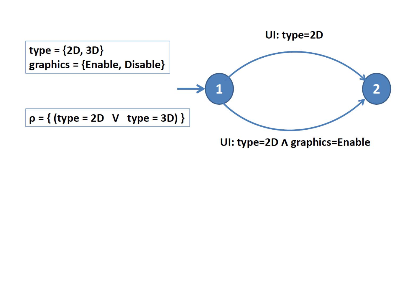
Similar to ECPL, we ran Algorithm 1 on all the 25 features of BSPL. In section 4, Figure 10 presents the number of design configurations and execution time of Algorithm 1 for each feature. In the following, we elaborate on the FSMv of 2 features: (i) User Interface and (ii) Withdraw Money. The FSMd/FSMr for all the features has states between 2 and 10 (both inclusive). Figure 8 is the FSMr for feature , which has as an event with global predicate . There is only one boolean variable, , takes values from .

Figure 9 is the FSMd for feature . This FSMd shares the event with the FSMr and has global predicate . There are two variables, , takes values from , while takes values from .
The analysis results for the two case studies are summarized in Figures 11 and 10 which gives the times taken by Algorithm 1. The number of product variants and the time taken for Algorithm 1 are very small in both case studies. In the case of ECPL, a bug was found in the feature 22 2 In , the transition from the middle elliptical state to the round state labeled with is incorrect; . Removing this transition fixes the bug.. In this case, after fixing the bug, for the second step we used SPIN which took 11 seconds. For BSPL, the second step was performed using the QBF approach and CirQit took just 0.005 seconds.
| Sr. No. | Features | Design Variants | SPIN Time(Sec) |
|---|---|---|---|
| 1 | UserInterface | 6 | 0.002 |
| 2 | CheckingBalance | 3 | 0.003 |
| 3 | WithdrawMoney | 8 | 0.027 |
| 4 | DepositMoney | 2 | 0.002 |
| 5 | PrintingStatement | 3 | 0.002 |
| 6 | Login | 1 | 0.001 |
| 7 | ATMLogin | 1 | 0.001 |
| 8 | ChangeAccountPassword | 2 | 0.003 |
| 9 | PayBills | 2 | 0.003 |
| 10 | PrintingBalanceAfterWithdraw | 2 | 0.003 |
| 11 | CheckingMoneyExchangeRate | 2 | 0.003 |
| 12 | MoneyExchange | 2 | 0.004 |
| 13 | InternationalTransfer | 2 | 0.006 |
| 14 | LocalTransferToOtherBank | 1 | 0.004 |
| 15 | LanguageSelection | 2 | 0.001 |
| 16 | MobileTopUp | 2 | 0.002 |
| 17 | ChangeMaxLimitForWithdrawal | 1 | 0.003 |
| 18 | LocalTransferToSameBank | 3 | 0.003 |
| 19 | AddBeneficiary | 1 | 0.002 |
| 20 | RemoveBeneficiary | 1 | 0.002 |
| 21 | CreateDemandDraft | 2 | 0.003 |
| 22 | ChequeClearance | 1 | 0.003 |
| 23 | FastWithdrawal | 1 | 0.002 |
| 24 | CreditCardPayment | 2 | 0.002 |
| 25 | UpdateContactDetails | 2 | 0.004 |
| Features | PL & LDCL | PCU | DL | DU | AL | TSL |
| Design Variants | 8 | 3 | 4 | 7 | 3 | 8 |
| SPIN Time (Sec) | 0.436 | 0.031 | 0.046 | 0.109 | 0.015 | 0.218 |
In the automotive domain, really very large SPLs are constructed [23]. Before undertaking the task of modeling such large examples, in order to quickly determine the scalability of our approach, we generated many random SPLs with 5000 to 25,000 features. Each of the corresponding FSMr/FSMd has two variables (four variants), and to states. Similar to the ECPL and BSPL cases, SPIN took very little time (less than 0.5 seconds) for each (FSMr, FSMd) pair. The composite FSMr/FSMd, and hence the QBF formula has then 10,000 to 50,000 variables. As we can see from Figure 12, the the time taken for the largest example is 196.69 seconds which is quite efficient. Encouraged by this result, we plan to take up the large industrial case studies.
| Variables in FSMr/FSMd | 10000 | 20000 | 30000 | 40000 | 50000 |
|---|---|---|---|---|---|
| CirQit 3.1.7 time (Sec) | 4.47 | 25.77 | 65.67 | 119.49 | 196.69 |
6 Conclusion
This paper motivated the need for extending the classical design verification problem to evolving SPL in which features and variability information can be added incrementally. The novel aspects of the proposed work are: (i) it verifies that the variability at the design level conforms to that at the requirement level, (ii) it is compositional and (iii) it reduces the conformance checking problem to QBF sat solving. A prototype tool has been implemented and experimented with modest sized examples with encouraging results.
References
- [1] Benavides, D., Segura, S., Ruiz-Cortés, A.: Automated analysis of feature models 20 years later: a literature review. Information Systems 35(6) (2010)
- [2] Classen, A., Heymans, P., Schobbens, P.Y., Legay, A.: Symbolic model checking of software product lines. In: Proceedings of ICSE 2011. (2011) 321–330
- [3] Cordy, M., Classen, A., Perrouin, G., Heymans, P., Schobbens, P.Y., Legay, A.: Simulation relation for software product lines: Foundations for scalable model checking (to appear). In: Proceedings of ICSE 2012. (2012)
- [4] Czarnecki, K., Eisenecker, U.: Generative Programming: Methods, Tools, and Applications. Addison-Wesley Professional (2000)
- [5] Metzger, A., Pohl, K.: Variability management in software product line engineering. In: ICSE COMPANION ’07: Companion to the proceedings of the 29th International Conference on Software Engineering. (2007) 186–187
- [6] Holzmann, G.J.: The SPIN Model Checker: Primer and Reference Manual. Addison-Wesley Professional (2003)
- [7] Goultiaeva, A., Bacchus, F.: Exploiting qbf duality on a circuit representation. In: Proceedings of AAAI 2010. (2010)
- [8] Narwane, G.K., Krishna, S.N., Millo, J.V., S.Ramesh: Composotional verification of evolving software product lines. In: http://www.cse.iitb.ac.in/krishnas/TR2012.pdf. (2012)
- [9] Larsen, K.G., Nyman, U., Wasowski, A.: Modal i/o automata for interface and product line theories. In: Proceedings of ESOP 2007. (2007) 64–79
- [10] Raclet, J.B., Caillaud, B., Badouel, E., Legay, A., Benveniste, A., Passerone, R.: Modal interfaces: Unifying interface automata and modal specifications. In: Proceedings of EMSOFT 2009. (2009)
- [11] Fantechi, A., Gnesi, S.: Formal modeling for product families engineering. In: Proceedings of SPLC 2008. (2008) 193–202
- [12] Gruler, A., Leucker, M., Scheidemann, K.D.: Calculating and modeling common parts of software product lines. In: Proceedings of SPLC 2008. (2008) 203–212
- [13] Gomaa, H., Olimpiew, E.: Managing variability in reusable requirement models for software product lines. In: High Confidence Software Reuse in Large Systems. (2008) 182–185
- [14] Berg, K., Bishop, J., Muthig, D.: Tracing software product line variability: from problem to solution space. In: Proceedings of SAICSIT ’05. (2005) 182–191
- [15] Metzger, A., Pohl, K., Heymans, P., Schobbens, P.Y., Saval, G.: Disambiguating the documentation of variability in software product lines: A separation of concerns, formalization and automated analysis. In: Proceedings of RE 2007. (2007) 243–253
- [16] Riebisch, M., Brcina, R.: Optimizing design for variability using traceability links. In: Proceedings of ECBS 2008. (2008) 235–244
- [17] Krishnamurthi, S., Fisler, K.: Foundations of incremental aspect model-checking. ACM Trans. Softw. Eng. Methodol. 16(2) (2007) 39
- [18] Liu, J., Basu, S., Lutz, R.: Compositional model checking of software product lines using variation point obligations. Automated Software Engineering 18 (2011) 39–76
- [19] Cordy, M., Schobbens, P.Y., Heymans, P., Legay, A.: Behavioural modelling and verification of real-time software product lines. In: Proceedings of SPLC 2012. (2012) 66–75
- [20] Lauenroth, K., Metzger, A., Pohl, K.: Quality assurance in the presence of variability. Technical report, SSE, Institut fur Informatik und Wirtschaftsinformatik, univertitat Duisburg Essen (2011)
- [21] Gruler, A., Leucker, M., Scheidemann, K.D.: Modeling and model checking software product lines. In: Proceedings of FMOODS 2008. (2008) 113–131
- [22] Vardi, M.Y., Wolper, P.: An automata-theoretic approach to automatic program verification. In: Proceedings of LICS 1986. (1986) 322–331
- [23] Flores, R., Krueger, C., Clements, P.: Mega-scale product line engineering at general motors. In: Proceedings of SPLC 2012. (2012) 259–269