Global dynamics of the buffered chemostat
for a general class of response functions

The chemostat was introduced in the fifties as an experimental device to study the microbial growth on a limiting resource [35, 38]. It is also often used as a mean to reproduce situations where (limiting) nutrients are fed to micro-organisms, typically in a liquid medium, in natural ecosystems [19, 6] or anthropized environments [27]. More generally, the chemostat is largely used as a scientific investigation tool in microbial ecology [24, 51].

The mathematical model of the chemostat has been extensively studied (see e.g. [46]) and used as a reference model in microbiology [39], microbial ecology [11] or biotechnological industries such as the waste-water treatment [8]. More generally, the chemostat serves to describe resource-consumer relations, where the resource is supplied at a constant rate. However, in many applications, the assumption of perfectly stirred chemostats is, in general, too restrictive. In the eighties, the gradostat, as an experimental device composed of a set of chemostats of identical volume interconnected in series, was introduced to represent spatial gradient [31], in a marine environment [21] or to model rhizosphere [13]. It motivated several mathematical studies [49, 23, 10, 43, 54, 45, 20, 47, 14]. Similarly, an interest for series of bioreactors appeared in biochemical industry, with tanks of different volumes to be minimized [32, 22, 5, 18, 9]. In ecology, island models have been proposed since the late sixties [33] to study the effects of heterogeneous environments with more general patterns than serial ones. Several studies of prey-predator in patchy environments have been conducted since then [26, 1]. Comparatively, relatively few studies have considered non-serial interconnections for resource-consumer models or chemostats [44]. In natural reservoirs such as in undergrounds or ground-waters, a spatial structure with interconnections between several volumes is often considered, each of them being approximated as perfectly mixed tank. Those interconnections can be parallel, series or built up in more complex networks. To our knowledge, the influence of the topology of a network of chemostats on the overall dynamics has been sparsely investigated in the literature. However, the simple consideration of two interconnected habitats can lead to non-intuitive behaviors [48, 36, 41, 25] and influence significantly the overall performances [37, 16]. Recently, literature in ecology has raised the relevance of “source-sink” models for describing plants/nutrients interactions, and predicting ecosystems performances [29, 15, 30]. Those models are mathematically close to general gradostat models, but with a significant difference concerning the resources compartments, for which the input rate mechanisms (due to atmospheric depositions or rock alterations) are assumed to be independent of the nutrient leaching (and not modeled as a transport term as in hydrology or in chemostat-like models).

It is also well-known since the seventies that microbial growth can be inhibited by large concentrations of nutrient. Such inhibition can be modeled by non-monotonic response functions [2, 4] and lead to initial-condition dependent washout [3, 52, 28]. Non-monotonic response functions occur in predator-prey models, for instance, when the predation decreases due to the ability of the prey to better defend when their population get larger. This non-monotonic functional response could also lead to bi-stability and possible extinction of the predator [12, 53].

Several control strategies of the input flow were proposed in the literature to globally stabilize the chemostat [7, 17, 40, 42] but the ability of a spatial structure to passively stabilize such dynamics has not been yet studied (in [44] a general structure of networks of chemostats is considered but with monotonic growth rates, while in [50] non-monotonic functions are considered but for the serial gradostat only).

The present work considers a particular interconnection of two chemostats of different volumes, one being a buffer tank. To our knowledge, this spatial structure, that is neither serial nor parallel, has not yet been considered in the literature. This structure is analogous to refuges in patchy environments [1], but here both consumer and resource are present in each vessel. We prove that it is possible with such a configuration to obtain repulsive washout equilibrium, while any serial, parallel or single tank structures with the same total volume exhibits multi-stability. This result brings new insights into the role of spatial patterns in the stability of bio-conversion processes in natural environments, where buffers can occur such as in soil ecosystems. It has also potential implications for the design of robust industrial bio-processes.

The paper is organized as follows. Section 2 presents the hypotheses and the buffered configuration, comparing with serial and parallel interconnections. Section 3 studies the multiplicity of equilibria and their stability for such configurations, considering a general class of response functions (monotonic as well as non-monotonic). Section 4 discusses the biological and ecological implications of the results of Section 3 in terms of persistence of microbial species in a non-homogeneous environment, along with some industrial perspectives. Numerical simulations illustrate the results on an Haldane function in Section 5. All the proofs are postponed to the Appendix.

We consider the chemostat model with a single strain growing on a single limiting nutrient. The system is fed with nutrient of concentration $S_{in}$ with flow rate $Q$. The total volume $V$ is assumed to be constant (i.e. input and output flow rates are supposed to be identical). When the concentrations of nutrient (or substrate) and biomass, denoted respectively $S$ and $X$, are homogeneous, as it is the case in perfectly mixed tanks, the system can be modeled by the well-known differential equations:

where $\mu(\cdot)$ is the uptake function and $Y$ the yield coefficient of the transformation of nutrient into biomass. Without any loss of generality, we take $Y=1$ (at the price of changing $X$ in $YX$). For convenience, we define the dilution rate

We consider quite general uptake functions, that fulfill the following properties.

The usual uptake functions, such as the Monod function [35]

or the Haldane one [2]

fulfill theses hypotheses. Classically, we consider the set

that plays an important role in the determination of the equilibria of the system. Under Assumptions A1, the set $\Lambda(D)$ is either empty or an open interval that we denote

where $\lambda_{+}(D)$ can be equal to $+\infty$.

We recall from the theory of the chemostat model (see for instance [46]) that under Assumptions A1 there are three kinds of phase portrait of the dynamics (1), depending on the parameter $S_{in}$.

Notice that in case 2, the qualitative behavior of the growth can change radically depending on the initial condition.

The question we investigate in this paper is related to the assumption that the vessel is perfectly mixed, and to the role that a spatial structure could have on the stability of the dynamics. Consider the case for which the washout equilibrium is attracting in the chemostat model (cases 1 and 2 of Proposition 1). Furthermore, consider spatial configurations with the same input flow and residence time than the perfectly mixed case, i.e. with the same total volume $V$ and input flow $Q$. Then, one has the following property.

This Lemma shows that when a bacterial species cannot persist in a chemostat, from any or a subset of initial conditions, this property persists in at least one vessel of any serial or parallel interconnection of chemostats with the same total volume. In the present work, we study a different kind of spatial configuration with an asymmetry created by two interconnected volumes, one of them serving as a buffer (see Figure 1). We call these spatial configurations a “buffered chemostat”, to be compared with the “single chemostat”.

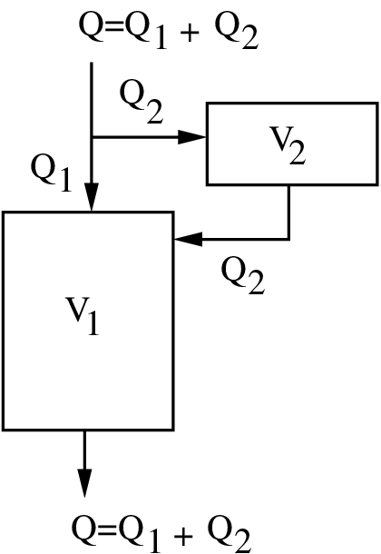
$V_{1}$ and $V_{2}$ are respectively the volumes of the main tank and the buffer, and $Q_{1}$ and $Q_{2}$ denote the input flow rates of each tank, with $Q=Q_{1}+Q_{2}$. We assume that each vessel is perfectly mixed. Straightforwardly, the dynamical equations of the buffered chemostat are

Notice that the limiting case $V_{1}=0$ consists in a by-pass of the volume $V_{2}$ with a flow $Q_{1}$.

In the next Section, we study the equilibria of this model, their multiplicity and their stability.

Given a volume $V$ and an input flow rate $Q$, we describe the set of all possible buffered configurations with $Q=Q_{1}+Q_{2}$ and $V=V_{1}+V_{2}$ by two parameters $r\in(0,1)$ and $\alpha>0$ defined as follows

This choice of parameterization is more convenient than the original one because it decouples more easily the role of the two parameters, as it is shown by equations (6) below.

Dynamics (5) can then be written in the following way

At equilibrium, one should have $\dot{S}_{2}+\dot{X}_{2}=\alpha D(S_{in}-S_{2}-X_{2})=0$ that is $S_{2}+X_{2}=S_{in}$. Then, one should have $\dot{S}_{1}+\dot{X}_{1}=D(S_{in}-S_{1}-X_{1})/r=0$ that is $S_{1}+X_{1}=S_{in}$. Thus, equilibria $(S_{1}^{\star},X_{1}^{\star},S_{2}^{\star},X_{2}^{\star})$ of dynamics (6) can be written as solutions of the following equations:

Due to the cascade structure of model (5), the study of the dynamics of the second reactor can be done independently of the first one. Depending of the value of $\alpha$, the three cases given in Proposition 1 for the single chemostat are possible in the second tank. This implies the following two possibilities for the equilibria of the first sub-system.

1. 1.

   When $(S_{2}(\cdot),X_{2}(\cdot))$ converges to the washout equilibrium (cases 1 and 2), the $(S_{1},X_{1})$ dynamics is asymptotically equivalent to a single chemostat model with dilution rate $D/r$, and Proposition 1 applies.

2. 2.

   When $(S_{2}(\cdot),X_{2}(\cdot))$ converges towards a positive equilibrium $(S_{2}^{\star}(\alpha),S_{in}-S_{2}^{\star}(\alpha))$ (cases 2 and 3), we consider the family of hyperbola $H_{\alpha,r}$ that are the graphs of the functions

   $$\phi_{\alpha,r}(s)=1+\frac{1-r}{r}\left(1-\alpha\frac{S_{in}-S_{2}^{\star}(\alpha)}{S_{in}-s}\right)$$

   (11)

   parameterized by $\alpha$ and $r\in(0,1)$. From equations (7) and (8), a positive equilibrium $(S_{1}^{\star},X_{1}^{\star})$ of (6) satisfies

   $$\phi_{\alpha,r}(S_{1}^{\star})=\mu(S_{1}^{\star})/D$$

   (12)

   or equivalently $S_{1}^{\star}$ is the abscissa of an intersection of the graph of $\mu(\cdot)/D$ with the hyperbola $H_{\alpha,r}$. Then, from equation (8), to each solution $S_{1}^{\star}$ corresponds a unique $X_{1}^{\star}=S_{in}-S_{1}^{\star}$. Notice that the washout is not an equilibrium for the first tank.

In the following, we consider only non-trivial cases for which the second tank admits a positive equilibrium, assuming the hypotheses:

Similar to the single chemostat that considers the set $\Lambda(D)$ given in (4), we define the set

We shall also consider the subset of configurations for which system (6) admits an unique positive equilibrium, denoted by

We state now our main results.

Let give some observations on these results.

• -

  In contrast to the single chemostat, for which the set $\Lambda(D)$ could be empty, the set $\Gamma_{\alpha,r}(D)$ is non-empty. This means that dynamics (6) always admits a positive equilibrium, even when the washout is the only equilibrium of the single chemostat, contrary to serial or parallel chemostats (cf Lemma 1).

• -

  When the initial condition of the $(S_{2},X_{2})$ sub-system belongs to the attraction basin of $(S_{in},0)$ (that could be reduced to a singleton), it is a not a surprise that the asymptotic behavior of the sub-system $(S_{1},X_{1})$ is the same as for a single chemostat with a dilution rate equal to $D/r$ (cf point i.). Otherwise, the whole state converges to a positive equilibrium, with a possible multiplicity of equilibria (cf point ii.). Here, a remarkable feature is the existence of buffered configurations $(\alpha,r)$ that possess an unique globally asymptotically stable equilibrium (when $\alpha D<\mu(S_{in})$ and $r\in\overline{R}_{\alpha}(D)$), in contrast to the single chemostat or any serial or parallel configurations for which a bi-stability occur when the functional response is non-monotonic.

To help grasp the geometric condition (12) that is the key for the characterization of the equilibria, we introduce the number

that fulfills the remarkable property

We first explicit the condition (12) on the specific case of the Haldane function (3):

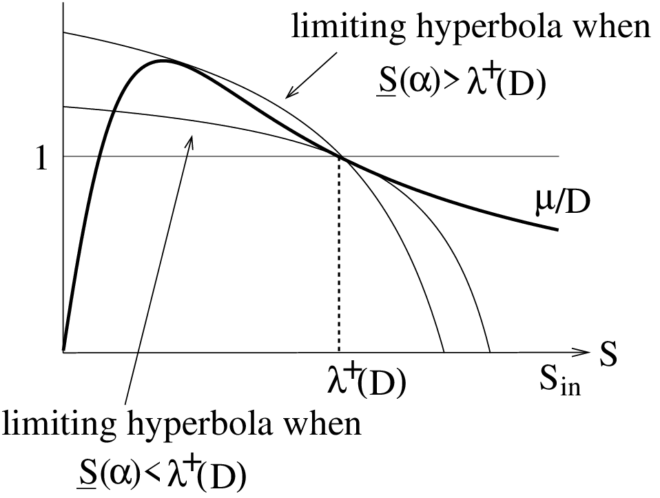
$S_{1}^{\star}$ is then a root of a polynomial $P$ of degree 3. So there exist at most three solutions of $\phi_{\alpha,r}(s)=\mu(s)/D$. For small values of $r$, we remark that $\phi_{\alpha,r}(0)$ is very large and $\phi_{\alpha,r}$ has a high slope. On the contrary, for $r$ near to $1$, $\phi_{\alpha,r}(0)$ is closed to $1$ and $\phi_{\alpha,r}$ has a light slope. Intuitively, we expect to have only one root for small values of $r$ and three for large values of $r$. For $\bar{r}$ such that there exists a solution $S_{1}^{\star}$ of $\phi_{\alpha,\bar{r}}(s)=\mu(s)/D$ and $\phi_{\alpha,\bar{r}}^{\prime}(s)=\mu^{\prime}(s)$, one has $P(S_{1}^{\star})=0$ and $P^{\prime}(S_{1}^{\star})=0$, that is $S_{1}^{\star}$ is a double root of $P$ (and there exists at most one such double root because $P$ is of degree 3). At such $S_{1}^{\star}$, the hyperbola $H_{\alpha,\bar{r}}$ is tangent to the graph of $\mu(\cdot)$. Intuitively, this corresponds to the limiting case for the parameter $r$ in between cases for which there is one or three roots (see Figures 2 and 3 where tangent hyperbola are drawn in thick line).

To formalize these observations for more general growth functions $\mu(\cdot)$ that fulfill Assumptions A1, we consider the set of $s$ at which the hyperbola $H_{\alpha,r}$ is tangent to the graph of the function $\mu(\cdot)/D$ and is locally on one side (that amounts to have $0$ as a local extremum of the function $\phi_{\alpha,r}(\cdot)-\mu(\cdot)/D$ at $s$):

along with the set

One can distinguish two cases:

1. 1.

   The single chemostat has only one attracting equilibrium. Tangencies of the graphs of $\phi_{\alpha,r}$ and $\mu$ could occur for certain values of $r$ (see Figure 3 as an illustration), leading to non-empty set $R_{\alpha}(D)$ and multi-equilibria. Another remarkable feature is that the buffer could create a multiplicity of equilibria.

2. 2.

   The single chemostat presents a bi-stability. The function $\mu$ is necessarily non-monotonic on $(0,S_{in})$ and a tangency of the graphs of $\phi_{\alpha,r}$ and $\mu$ always occurs for a certain $r$ with an abscissa that is located

   • -

     either at the right of $\lambda_{+}$ when $\underline{S}(\alpha)<\lambda_{+}(D)$ (see the right picture of Figure 2),

   • -

     either at the left of $\lambda_{+}$ when $\underline{S}(\alpha)>\lambda_{+}(D)$ (see the left picture of Figure 2).

In the Appendix, more properties on the sets $R_{\alpha}(D)$ and the multiplicity of equilibria are given in the Proposition 2.

In this Section, we discuss the applications of Theorem 1 in terms of ecological and biotechnological implications for different buffered configurations.

In this section, we illustrate numerically the stabilizing effect of a buffer. We consider the case of the single chemostat model that presents a bi-stability (see the discussion in 4.1.1), with a non-monotonic uptake function given by the Haldane expression (3). One can easily check that for this function the set $\Lambda(D)$ defined in (4) is non-empty exactly when the condition

is fulfilled. Then, $\lambda_{-}(D)$, $\lambda_{+}(D)$ are given by the following expressions:

Bi-stability occurs when the condition $S_{in}>\lambda_{+}(D)$ is fulfilled (case 2 of Proposition 1).

Recall from Section 3, that for the Haldane function, the solutions of the equation (12) are roots of a polynomial of order $3$ with at most three solutions of (16). There is a most one double root, which implies that the set ${\cal S}_{r,\alpha}(D)$ possesses at most one element. Proposition 2 (case II), given in the Appendix, helps to characterize the set $\overline{R}_{\alpha}(D)$ depending on the subsets $R^{-}_{\alpha}(D)$, $R^{+}_{\alpha}(D)$ that are defined in this Proposition:

• -

  the set $R^{+}_{\alpha}(D)$ is a singleton, because there are at most three equilibria,

• -

  $R^{-}_{\alpha}(D)\cap R^{+}_{\alpha}(D)=\emptyset$ because ${\cal S}_{r,\alpha}(D)$ possesses at most one element,

• -

  when $R^{-}_{\alpha}(D)$ is non-empty, one has $\max R^{-}_{\alpha}(D)<\min R^{+}_{\alpha}(D)$: for any $r\in(\min R^{-}_{\alpha}(D),\max R^{-}_{\alpha}(D))$, equation (12) has at least three solutions on an interval $I$, and for $r\in(\min R^{+}_{\alpha}(D),1)$ at least two on another interval $J$, where $I$ and $J$ are disjoint. If $\max R^{-}_{\alpha}(D)\geq\min R^{+}_{\alpha}(D)$, there would exist at least five solutions of equation (12) on $(0,S_{in})$.

We study now the set of “stable” buffered configurations ${\cal C}_{D}$ as the set of pairs $(\alpha,r)$ such that the buffered chemostat model admits a unique positive equilibrium. The upper boundary of ${\cal C}_{D}$ is thus given by the curve

where $\bar{r}_{D}(\alpha)$ is the single element of the set $R^{+}_{\alpha}(D)$. Notice that the limiting case $\alpha D=\mu(S_{in})$ can have also global stability (see Lemma 2 in the Appendix). The number $\bar{r}_{D}(\alpha)$ can then be determined numerically as the unique minimizer of the function

on $(0,1)\times\{s\in(\lambda^{-}(D),S_{in})\mbox{ s.t. }(s-\lambda^{+}(D))(\lambda^{+}(D)-\underline{S}(\alpha))\geq 0\}$ that is, for the Haldane function:

where $\underline{S}(\alpha)$ is defined in (15). For the parameters given in Table 1, we have computed numerically the domains ${\cal C}_{D}$ for different values of $S_{in}$, depicted on Figure 4.

One can see that the map $\alpha\mapsto\bar{r}_{D}(\alpha)$ is discontinuous at $\alpha=\underline{\alpha}$, where $\underline{\alpha}$ is such that $\underline{S}(\underline{\alpha})=\lambda_{+}(D)$ (when it exists), as mentioned in Remark 1. On Figure 5 one can see that the two limiting hyperbolas $H_{\alpha,\bar{r}(\alpha)}$ about $\underline{\alpha}$ are different in a such a case.

So, this study reveals the role of the input concentration $S_{in}$ on the shape of the domain ${\cal C}_{D}$.

Finally, we have compared the two scenarios discussed in 4.2 for improving the stability of the single chemostat, by enlarging its volume or adding a buffer, given respectively by formulas (20) and (32). For the parameters given in Table 1, the numerical comparison is reported on Figure 6 as a function of the input concentration $S_{in}$.

As expected, the buffered chemostat requires less volume augmentation, but one can also discover that this advantage becomes more significant as the input concentration $S_{in}$ is higher. Finally, this study demonstrates on a concrete example the flexibility of the buffered chemostat in the choice of possible configurations, with two parameters to be tuned (instead of one for the single chemostat).

The present analysis illustrates how the addition of a buffer to chemostat alters the multiplicity and stability of their equilibria. This property has several impacts on theoretical ecology as well as for bio-industrial applications.

• -

  From an ecological viewpoint, a spatial pattern with a buffer can explain why a species can persist in an environment that is unfavorable if it was perfectly mixed. On the opposite, the emergence of a buffer with particular characteristics can destabilize a regime that is stable under perfectly mixed conditions, and could lead to the extinction of the species. Nevertheless, such a case occurs only for “fragile” species with non-monotonic response function.

• -

  For industrial applications, such as waste-water purification or pharmaceutic production, a buffered configuration of two tanks, instead of one or serial or parallel interconnections, present several advantages when there is an inhibition in the growth rate. It provides an easy and robust way to prevent the washout of the biomass in the process, without requiring upstream storage or real-time controller.

The numerical study has also revealed other interesting characteristics of the buffered chemostat. First, the size of the “buffer” or the additional tank that provide such properties could be relatively small. Secondly, the shape of the set of buffered configurations that provide a unique (globally asymptotically stable) positive equilibrium depends on the density of the supplied resource, with a threshold that makes this shape non smooth.

Finally, those results provide new insights on the role of spatial structures in resource/consumer models for natural ecosystems, and new potential strategies for the design of industrial bioprocesses. Of course, more complex interconnections could be considered, with for instance an additional output from the buffer. However, the main contribution of the present work is to show that a simple configuration with only two parameters can change radically the overall dynamic behavior. The buffered chemostat appears to be the simplest pattern that can provide global stability, while any serial or parallel configurations cannot do.

Our study considered a single strain. According to the Competitive Exclusion Principle, it is not (generically) possible to have more than one species persisting in the buffer tank, but this does not prevent to have coexistence with another species in the main tank, which is not possible with a single chemostat. Consequently, it might be relevant to study the dynamics of the buffered chemostat with different persistent species in the buffer and in the main tank.

The authors are grateful to INRA and INRIA supports within the French VITELBIO (VIRtual TELluric BIOreactors) research program. The authors thank also Prof. Denis Dochain, CESAME, Univ. Louvain-la-Neuve, for fruitful discussions. The authors would also like to thank the anonymous referees for their relevant suggestions for improvements of our initial work.

Proof of Lemma 1.

In the serial connection, the dynamics of the first tank of volume $V_{1}$ is given by equations (1) where $V$ is replaced by $V_{1}\leq V$. Its dilution rate is then equal to $Q/V_{1}$, that is greater than $Q/V$ and consequently one has $S_{in}\notin\Lambda(Q/V_{1})$. According to Proposition 1, only Cases 1 or 2 can occur in the first tank.

In the parallel connection, the dynamics of each tank of volume $V_{i}$ and flow rate $Q_{i}$ is given by equations (1) where $V$ and $Q$ are replaced by $V_{i}$ and $Q_{i}$. Denote $r_{i}=V_{i}/V$ and $\alpha_{i}=Q_{i}/Q$, and notice that one has $\sum_{i}r_{i}=\sum_{i}\alpha_{i}=1$. Then, the dilution rate $D_{i}$ in the tank $i$ is equal to $\alpha_{i}/r_{i}D$. According to Proposition 1, a necessary condition for having the washout equilibrium repulsive in each tank is to have $D_{i}<D$ for any $i$, that is $\alpha_{i}<r_{i}$, which contradicts $\sum_{i}r_{i}=\sum_{i}\alpha_{i}=1$. $\Box$

Before giving the proof of Theorem 1, we present in the next proposition a series of results concerning the multiplicity of equilibria and the characterization of the sets $\overline{R}_{\alpha}(D)$ defined in (14).

References

- [1] P. Amarasekare and R. Nisbet, Spatial heterogeneity, source‐sink dynamics, and the local coexistence of competing species, The American Naturalist, 158(6) (2001), 572–584.
- [2] J.F. Andrews, A mathematical model for the continuous culture of microorganisms utilizing inhibitory substrates, Biotech. Bioengrg., 10 (1968), 707–723.
- [3] G. J. Butler and G. S. K. Wolkowicz, A mathematical model of the chemostat with a general class of functions describing nutrient uptake, SIAM J. Appl. Math. 45 (1985), 138–151.
- [4] A. Bush and A. Cook The effect of time delay and growth rate inhibition in the bacterial treatment of wastewater J. Theor Biol. 63(2) (1976), 385–395.
- [5] C. de Gooijer, W. Bakker, H. Beeftink and J. Tramper, Bioreactors in series: An overview of design procedures and practical applications, Enzyme and Microbial Technology, 18 (1996), 202–219.
- [6] E. Di Mattia, S. Grego and I. Cacciari, Eco-physiological characterization of soil bacterial populations in different states of growth Microb. Ecol. 43(1) (2002), 34–43.
- [7] D. Dochain and G. Bastin Adaptive identification and control algorithms for non linear bacterial growth systems. Automatica, 20(5) (1984), 621–634.
- [8] D. Dochain and P. Vanrolleghem, Dynamical Modelling and Estimation in Wastewater treatment Processes, IWA Publishing, U.K. (2001).
- [9] A. Dramé, J. Harmand, A. Rapaport and C. Lobry, Multiple steady state profiles in interconnected biological systems, Mathematical and Computer Modelling of Dynamical Systems, 12 (2006), 379–393.
- [10] H. El-Owaidy and O. El-Leithy, Theoretical studies on extinction in the gradostat Mathematical Biosciences, 101(1) (1990), 1–26.
- [11] A. Fredrickson and G. Stephanopoulos, Microbial Competition Science, 213 (1981), 972–979.
- [12] H. Freedman and G. Wolkowicz, Predator-prey systems with group defence: The paradox of enrichment revisited. Bulletin of Mathematical Biology, 48(5/6) (1986) 493–508.
- [13] C. Fritzsche, K. Huckfeldt and E.-G. Niemann, Ecophysiology of associative nitrogen fixation in a rhizosphere model in pure and mixed culture, FEMS Microbiology Ecology, 8(4) (2011), 279–290.
- [14] A. Gaki, Al. Theodorou, D. Vayenas and S. Pavlou, Complex dynamics of microbial competition in the gradostat, Journal of Biotechnology, 139(1) (2009) pp 38–46.
- [15] D. Gravel, F. Guichard, M. Loreau and N. Mouquet, Source and sink dynamics in metaecosystems. Ecology, 91 (2010), 2172–2184.
- [16] I. Haidar, A. Rapaport and F. Gérard, Effects of spatial structure and diffusion on the performances of the chemostat, Mathematical Biosciences and Engineering, 8(4) (2011), 953–971.
- [17] J. Harmand, A. Rapaport and F. Mazenc, Output tracking of continuous bioreactors through recirculation and by-pass, Automatica, 42(7) (2006) 1025–1032.
- [18] J. Harmand, A. Rapaport and A. Trofino, Optimal design of two interconnected bioreactors–some new results, American Institute of Chemical Engineering Journal, 49 (1999), 1433–1450.
- [19] A. Hasler and W. Johnson, The in situ chemostat – a self-contained continuous culturing and water sampling system. Limnol. Oceanogr. 79 (1954), 326–331.
- [20] J. Hofbauer and W. So, Competition in the gradostat: the global stability problem Original Research Nonlinear Analysis: Theory, Methods & Applications, 22(8) (1994), 1017–1031.
- [21] Y. Higashi, N. Ytow, H. Saida and H. Seki, In situ gradostat for the study of natural phytoplankton community with an experimental nutrient gradient Environmental Pollution, 99 (1998), 395–404.
- [22] G. Hill and C. Robinson, Minimum tank volumes for CFST bioreactors in series, The Canadian Journal of Chemical Engineering, 67 (1989), 818–824.
- [23] W. Jaeger, J.-H. So, B. Tang and P. Waltman, Competition in the gradostat, J. Math. Biol. 25 (1987), 23–42.
- [24] H. Jannash and R. Mateles, Experimental bacterial ecology studies in continuous culture, Advanced in Microbial Physiology 11 (1974), 165–212.
- [25] P. Lenas, N. Thomopoulos, D. Vayenas and S. Pavlou, Oscillations of two competing microbial populations in configurations of two interconnected chemostats, Mathematical Biosciences, 148(1) (1998), 43–63.
- [26] S. Levin, Dispersion and population interactions, The American Naturalist, 108(960) (1974), 207–228.
- [27] J. La Rivière, Microbial ecology of liquid waste, Advances in Microbial Ecology, 1 (1977), 215–259.
- [28] B. Li, Global asymptotic behavior of the chemostat: General response functions and differential removal rates, SIAM J. Appl. Math. 59 (1998), 411–22.
- [29] M. Loreau, From Populations to Ecosystems: Theoretical Foundations for a New Ecological Synthesis. Princeton University Press, Princeton (2010).
- [30] M. Loreau, T. Daufresne, A. Gonzalez, D. Gravel, F. Guichard, S.J. Leroux, N. Loeuille, F. Massol and N. Mouquet. Unifying sources and sinks in ecology and Earth sciences. Biological Review 88 (2013), 365–79.
- [31] R. Lovitt and J. Wimpenny, The gradostat: A bidirectional compound chemostat and its applications in microbial research, Journal of General Microbiology, 127 (1981), 261–268.
- [32] K. Luyben and J. Tramper, Optimal design for continuously stirred tank reactors in series using Michaelis-Menten kinetics, Biotechnology and Bioengineering, 24 (1982), 1217–1220.
- [33] R. MacArthur and E. Wilson, The Theory of Island Biogeography, Princeton University Press (1967).
- [34] M. Mischaikow, H. Smith and H. Thieme, Asymptotically autonomous semiflows: chain recurrence and Lyapunov functions, Transactions of the American Mathematical Society, 347(5) (1995), 1669–1685.
- [35] J. Monod, La technique de la culture continue: Théorie et applications, Annales de l’Institut Pasteur, 79 (1950), 390–410.
- [36] S. Nakaoka and Y. Takeuchi, Competition in chemostat-type equations with two habitats, Mathematical Bioscience, 201 (2006), 157–171.
- [37] M. Nelson and H. Sidhu, Evaluating the performance of a cascade of two bioreactors, Chemical Engineering Science, 61 (2006), 3159–3166.
- [38] A. Novick and L. Szilard, Description of the chemostat, Science, 112 (1950), 715–716.
- [39] J. Pirt, Principles of Microbe and Cell Cultivation, Blackwell Scientific Publications (1975).
- [40] A. Rapaport and J. Harmand, Biological control of the chemostat with non-monotonic response and different removal rates, Mathematical Biosciences and Engineering, 5(3) (2008), 539–547.
- [41] A. Rapaport, J. Harmand and F. Mazenc, Coexistence in the design of a series of two chemostats, Nonlinear Analysis, Real World Applications, 9 (2008), 1052–1067.
- [42] A. Schaum, J. Alvarez and T. Lopez-Arenas, Saturated PI control of continuous bioreactors with Haldane kinetics Chem. Eng. Science, 68 (2012), 520–529.
- [43] H. Smith and B. Tang, Competition in the gradostat: the role of the communication rate, J. Math. Biol. 27(2) (1989), 139–165.
- [44] H. Smith, B. Tang and P. Waltman, Competition in an n-vessel gradostat, SIAM J. Appl. Math. 51 (1991), 1451–1471.
- [45] H. Smith and P. Waltman, H.L. Smith, P. Waltman, The gradostat: a model of competition along a nutrient gradient, J. Microb. Ecol. 22 (1991), 207–226.
- [46] H. Smith and P. Waltman, The theory of chemostat, dynamics of microbial competition, Cambridge Studies in Mathematical Biology, Cambridge University Press (1995).
- [47] H. Smith and P. Waltman, Competition in the periodic gradostat, Nonlinear Analysis: Real World Applications, 1(1) (2000), 177–188.
- [48] G. Stephanopoulos and A. Fredrickson, Effect of inhomogeneities on the coexistence of competing microbial populations, Biotechnology and Bioengineering, 21 (1979), 1491–1498.
- [49] B. Tang, Mathematical investigations of growth of microorganisms in the gradostat, J. Math. Biol. 23 (1986), 319–339.
- [50] B. Tang, Competition models in the gradostat with general nutrient uptake functions, Rocky Mountain J. Math. 24(1) (1994), 335–349.
- [51] H. Veldcamp, Ecological studies with the chemostat, Advances in Microbial Ecology, 1 (1977), 59–95.
- [52] G. Wolkowicz and Z. Lu, Global dynamics of a mathematical model of competition in the chemostat: general response functions and differential death rates, SIAM J. Appl. Math. 52 (1992), 222–233.
- [53] D. Xiao and S. Ruan, Global analysis in a predator-prey system with nonmonotonic functional response. SIAM Journal on Applied Mathematics, 61(4) (2001), 11445–72.
- [54] A. Zaghrout, Asymptotic behavior of solutions of competition in gradostat with two limiting complementary substrates Applied Mathematics and Computation, 49 (1) (1992), 19–37.