Exoplanets Beyond the Solar Neighbourhood: Galactic Tidal Perturbations
Abstract
The majority of Milky Way extrasolar planets likely reside within a few kpc of the Galactic centre. The Galactic tidal forces acting on planets scale inversely with radius in the Galaxy and so are much greater in the inner Galaxy than in the Solar neighbourhood. Within a range of 3.5 to 10 kpc, the vertical tide from the Galactic disc is predominant. Interior to 3.5 kpc, the effects of the Galactic bulge cannot be neglected and the in-plane tidal components are as important as the vertical ones. Here, we quantify the orbital changes induced by these tides. We find that the greatest perturbations occur when the planetary orbit is severely misaligned to the parent star’s orbit. When both planes are perpendicular, the eccentricity of the planet is driven to unity, although the semimajor axis is secularly unaffected. When both planes are coincident, the effect from Galactic tides is minimized, but remains non-zero. In these cases, we provide estimates for the survival times, as well as the minimum baseline eccentricity variation for all Milky Way exoplanets as a function of Galactic parameters. Inclinations similar to the Solar System’s () can easily cause eccentric Neptunes (at AU) around host stars deep within the Galactic bulge (within pc) to experience eccentricity variations of several tenths, and cause the exoplanets with the widest-known separations ( AU) to experience similar variations in the Galactic disc. These variations occur on timescales of a few Gyr, a fraction of a typical main sequence lifetime.
Keywords:
planets and satellites: dynamical evolution and stability – planet-star interactions – fundamental parameters; The Galaxy: kinematics and dynamics – structure – disc1 Introduction
The vast majority of the thousands of candidate and confirmed exoplanets reside in the Solar neighborhood 11 1 See the Extrasolar Planet Encyclopedia at http://exoplanet.eu/,22 2 See the Exoplanet Data Explorer at http://exoplanets.org/, which is kpc from the Galactic centre. Given their abundance locally, it is natural to conclude that the whole Galaxy is teeming with exoplanets, in accord with the Copernican Principle. Some confirmation is provided by microlensing surveys, which typically monitor source stars in the Galactic bulge. Intervening host stars can act as gravitational lenses, whilst their associated exoplanets can be detectable as perturbations of the microlensing lightcurves (Dong et al., 2009; Janczak et al., 2010; Miyake et al., 2011; Yee et al., 2012, e.g.). In this way, exoplanets have been discovered at Galactocentric radii from to kpc, as exemplified by OGLE 2007-BLG-050 (Batista et al., 2009) and OGLE-2003-BLG-235 (Bennett et al., 2006). Additionally, the SWEEPS (Sagittarius Window Eclipsing Extrasolar Planet Search) collaboration identified 15 transiting exoplanet candidates in the Galactic bulge, and concluded planets are just as common there as in the Solar neighbourhood (Sahu et al., 2006).
The density of the Galactic disc increases moving towards the centre in a roughly exponential manner with a scale length of between 2 and 3 kpc (Binney & Merrifield, 1998, see e.g.,). Additionally, the innermost parts of the Milky Way are dominated by a boxy-shaped bulge, as seen most prominently in the COBE/DIRBE near-infrared light distributions (Dwek et al., 1995). As the star density increases substantially towards the centre, there are many more possible exoplanet hosts in the inner Galaxy than in the remoter outskirts, like the Solar neighbourhood. However, the Galactic environment itself becomes more extreme, as stellar collisions, encounters, and flybys are more frequent in the inner parts and the Galactic tides are stronger.
The largest component of the Galactic tidal field in the Galactic disc acts perpendicular to the Galactic plane. Unfortunately, observations have not yet been able to identify a typical planetary orbit inclination with respect to the Galactic plane due to a strong bias: the majority of all exoplanetary candidates have been discovered by the Kepler mission (Borucki et al., 2011a; Borucki et al., 2011b; Batalha et al., 2012), which observes a fixed patch of sky along the Orion arm and can detect candidates with only nearly edge-on orbits. Programs to detect transiting planets see them edge-on at a wide variety of declinations and right ascensions, depending on the instruments’ line of sights (see Veras & Moeckel 2012 for a more detailed discussion). The radial velocity technique, which is responsible for the discovery of the majority of confirmed exoplanets, provides no information about the planetary orbital inclination with respect to the Galactic centre. Further, the Solar System’s invariable plane and ecliptic are misaligned with the Galactic plane at an angle of approximately (Huang & Wade, 1966; Duncan et al., 1987, e.g.). Although the Galactic inclination distribution of exoplanets is unconstrained, high inclinations certainly exist, and may even be typical.
Regardless of their orientation and location in the Galaxy, all Milky Way exoplanetary systems experience the Galactic tide. Within its Hill or Roche surface, a star’s gravity dominates and an exoplanet may survive the effects of Galactic tides unscathed (Heisler & Tremaine, 1986, e.g.,). Exterior to the Hill surface, the Galactic tides are always important. For a star in the Solar neighbourhood, the Hill surface has an extent AU, which is a measure of the size of any exoplanetary system. At a Galactocentric radius of 500 pc, the Hill surface is an order of magnitude smaller with a typical extent of AU. For the planets in the Solar system, the Galactic tide is not generally important. Although effects of tides on planets in the Solar neighbourhood has been considered before, studies of tides on exoplanetary systems in the bulge has been restricted to Oort clouds (Brasser et al., 2010).
A rough rule-of-thumb is that the precession timescale due to tides , where is the orbital period of the host star in the Galaxy and is the orbital period of the planet around the star. For Jupiter, this gives yr, well in excess of a Hubble time. However, wide-separation planets are now known (Goldman et al., 2010; Luhman et al., 2011; Kuzuhara et al., 2011, see e.g.,) with semimajor axes up to AU. For such wide-separation planets in the inner Galaxy, yr or less. In other words, there can be significant effects from Galactic tides over the age of such exoplanetary systems.
1.1 Wide Orbit Planet Motivation
Given the observationally-motivated emphasis in this work on wide-orbit planets, here we provide an updated summary of Veras et al. (2009), which describes the prospects for the formation, survival and detection of these bodies.
1.1.1 Formation of Wide-Orbit Planets
Here we briefly review mechanisms for generating planets at different distances from their host stars. The core accretion formation mechanism (Pollack et al., 1996, e.g.) can readily form planets at several AU but has difficulty forming planets at tens of AU. Even Uranus and Neptune, at AU and AU, require particularly favorable circumstances to have been formed in situ from core accretion (Levison & Stewart, 2001; Thommes et al., 2002). Dodson-Robinson et al. (2009) claim that AU is a rough limit beyond which massive gas giant planets must form by an alternate mechanism, such as gravitational instability in the disc (Cameron, 1978; Boss, 1997, e.g.); Boley (2009) claims that this limit is approximately AU. Disc instability easily forms planets at tens of AU (Boss, 2003; Boss, 2011), and may or may not be able to form planets at a couple hundred AU (Boss, 2006; Boley, 2009).
Beyond a few hundred AU, planets are highly unlikely to have been formed in situ. Instead, they were likely formed and subsequently scattered outward within the same system due to multi-planet gravitational instability (Rasio & Ford, 1996; Weidenschilling & Marzari, 1996; Lin & Ida, 1997, e.g.). Scharf & Menou (2009) and Veras et al. (2009) showed that planet-planet scattering amongst massive gas giants which could have been formed by core accretion ( AU) may generate a population of planets from AU - AU. However, those planets with the widest orbits are unlikely to remain bound for several tens of Myr if they interact with any surviving tight-orbit planets. Boley et al. (2012) performed multi-planet scattering studies assuming one planet was formed by gravitational instability at AU. This initial wide-orbit planet induced significant radial mixing, ultimately producing a population of planets with separations between several hundred and several thousand AU (see their Fig. 15). Alternatively, wide-orbit planets could represent captured free-floaters (Perets & Kouwenhoven, 2012; Varvoglis et al., 2012), a possibility that will become increasingly plausible with additional studies that support the purported vast free-floating planet population (Sumi et al., 2011).
1.1.2 Survival of Wide-Orbit Planets
Planets scattered to stable wide orbits could remain in those orbits if they remain unperturbed. One potential destabilizing perturbative source is a remnant inner planet which survives the scattering phase. If the wide-orbit planet is sufficiently eccentric, then repeated perturbations by the inner planet will cause an additional scattering event and instability. This additional scattering event may not take place for tens of Myr (Veras et al., 2009).
Another perturbative source is the birth cluster itself. Although stellar flybys can actually aid the passage of a planet onto a wide orbit (Malmberg et al., 2011; Boley et al., 2012, e.g.), alternatively flybys could also cause instability and ejection. Adams et al. (2006) estimate that over 10 Myr, for clusters with between 100-1000 members, the typical impact parameter for two stars passing each other is about 700-4000 AU. Any planets at or beyond these distances are likely to be severely disrupted. Whether this disruption triggers ejection or just a shift to a different wide orbit is dependent on the geometry of the encounter (Veras & Moeckel, 2012, see, e.g.). Planets with tighter orbits also may experience instabilities with a wide range of outcomes; recently Parker & Quanz (2012) performed 10 Myr cluster simulations with single planets on circular orbits at 5 and 30 AU, and found escape, orbit disruption, or quiescent evolution were all possible outcomes for individual stellar systems.
Overall then planetary interaction in clusters is highly model-dependent and disrupted planets may or may not survive cluster evolution on wide orbits. A simpler argument for how planets can survive their birth cluster evolution is that in many cases the dissociation timescale for the cluster is much shorter than the timescale for a planet to experience a strong perturbation from a stellar flyby, or even fully form. Although the cluster dissociation timescale is a function of both gas dynamics as well as N-body dynamics (Moeckel et al., 2012, e.g.), the dissociation timescale appears to be positively correlated with the cluster membership population (e.g. Sterzik & Durisen, 1995; Bate, 2012, and references therein). Therefore, the smaller the cluster, the more likely planets can survive the cluster phase undisturbed.
1.1.3 Detection of Wide-Orbit Planets
Although the majority of exoplanets have been discovered with Doppler radial velocity variations or transit measurements, these techniques fail to probe the outer reaches of planetary systems. The widest-orbit planets are instead discovered by direct high-contrast imaging. These detections often require follow-up imaging studies at different wavelengths and/or with different instruments to ensure that the star and companion are kinematically associated with each other (have the same proper motion) and to constrain the companion’s mass. For example, the exoplanet with the widest-known orbit (a projected separation of AU), WD 0806-661B b, was initially detected by Luhman et al. (2011) but was later confirmed by Luhman et al. (2012).
All 16 companions at separations of at least 100 AU from their parent stars33 3 Numbers are correct as of 18 November 2012 from the Extrasolar Planets Encyclopedia. have super-Jovian masses, and at least half of these are likely to be brown dwarfs by mass (Spiegel et al. 2011 show the planet/brown-dwarf boundary to be ). For WD 0806-661B b, the companion’s mass is reported as , safely pinpointing this companion as a planet. Although the distinction between planetary masses and brown dwarf masses likely helps to indicate the way the objects are formed, the resulting difference in motion due to Galactic tides is negligible.
Probing this super-Jovian mass regime is important for understanding the low-mass tail of the initial mass function and evaluating the extent of the brown dwarf desert (Marcy & Butler, 2000; Grether & Lineweaver, 2006; Deleuil et al., 2008; Pinfield et al., 2012). Further, exploring planetary systems beyond about AU is important for comparison with the Solar System, and to assess the prevalence of exo-Kuiper belts and exo-Oort clouds (Raymond & Armitage, 2012, e.g.). The Gemini Planet Imager (GPI), with first light due in January 2013, is dedicated to exploring outer regions of exosystems where radial velocity and transit surveys cannot reach. Forthcoming GPI discoveries will raise questions about the formation and fate of wide-orbit companions, and are likely to revise the current Galactic-wide exoplanet population estimates (Sumi et al., 2011; Cassan et al., 2012). Our study helps to preempt this line of inquiry by considering the effect of Galactic tides on wide-orbit companions at all distances within the Solar Circle.
1.2 Plan for Paper
This paper examines how the Galactic tidal field may drive orbital evolution in exoplanets for disc and bulge host stars. We first rederive the equations of planetary motion subject to the Galactic tidal field in Section 2. We build a new three-component model of the Galaxy in Section 3 and demonstrate the relative importance of each component in different regions. We apply these equations in the regions dominated by the Galactic disc (Section 4) and Galactic bulge (Section 5) before characterising the minimum-possible eccentricity variation of exoplanets due to tides throughout the entire Milky Way in Section 6. We discuss these results in Section 7 and conclude in Section 8.
2 The Galactic Tides
2.1 Derivation
The disturbances on a planetary orbit can be modeled with the perturbed two-body problem. Following Heisler & Tremaine (1986), we use a non-rotating, rectangular coordinate system centered on, and orbiting with, the host star. The star is assumed to move on a circular orbit of radius about the Galactic centre with frequency . Then the instantaneous unit vectors in the radial and tangential directions are
| (1) | |||||
| (2) |
The triad () has fixed spatial directions while () rotates with the star. At the origin of both primed and unprimed coordinate systems, the gravitational force from the Galactic potential exactly balances the centripetal force for circular motion
| (3) |
At a general point in the exoplanetary system, the force per unit mass is the sum of the forces derived from the two-body problem of star and planet, the forces due to the rest of the Galaxy, and the fictitious forces caused by our choice of a non-inertial frame:
| (4) |
Now, we Taylor expand the Galactic potential about the host star’s position to obtain
| (5) | |||||
This expansion implies further that
| (6) | |||||
If the host star lies in the Galactic plane, then the approximate symmetry of the Galactic potential ensures that the vertical gradient vanishes. It is conventional to introduce the Oort constants
| (7) | |||||
| (8) |
which gives us
| (9) | |||||
Finally, we can use Poisson’s equation in cylindrical coordinates to relate the local density at the host star to the vertical gradients:
| (10) |
We thus obtain an equation derived by Heisler & Tremaine (1986),
| (11) | |||||
By converting from the primed to the unprimed coordinate system, this equation takes the form
| (12) | |||||
| (13) | |||||
| (14) |
where and represent the masses of the star and planet, respectively, and the perturbations are
| (15) | |||||
| (16) | |||||
| (17) | |||||
| (18) | |||||
| (19) |
where . This form of the equations is given in Brasser et al. (2010)44 4 There is a sign error in their expression for , although our derivation makes it clear that the reference frame is not inertial, as they mistakenly claim. For any Galactic model, the Oort constants and , together with the shear , are calculable from the Galactic potential and vary with position in the Galaxy.
2.2 Perturbative Equations of Motion
The perturbed two-body problem is usually written down in terms of orbital elements, which provide greater intuition into how the size and shape of a Keplerian ellipse changes under the perturbations. We can express the equations of motion (12)-(14) in terms of orbital elements by using Gauss’ theory or Lagrange’s equations (Burns 1976 and pgs. 54-57 of Murray & Dermott 1999). An alternative procedure for deriving the orbital equations subject to very general perturbative forces has been given recently by Veras & Evans (2012).
A commonly-used approximation in non-linear systems is to separate the fast and slow oscillation variables. In celestial mechanics, this procedure can be performed by averaging over the fast oscillations of the mean anomaly or true anomaly of the orbiting body. The result is averaged equations for the evolution of the more slowly oscillating variables, such as the semimajor axis or eccentricity. This “adiabatic” approximation is valid when , where is the mean motion of the planet. Effectively, for the Milky Way, this relation holds whenever the semimajor axis AU.
In the general case, a planetary orbit is not coplanar with the Galactic disc. In the Solar neighbourhood, the out-of-plane tidal component is an order of magnitude greater than the in-plane components. Thus, the vertical tide usually dominates the motion, unless the inclination is very low. This approximation has been used to simplify the equations in many previous studies (Heisler & Tremaine, 1986; Matese & Whitman, 1989; Matese & Whitman, 1992; Matese et al., 1995; Breiter et al., 1996; Brasser, 2001; Breiter & Ratajczak, 2005). The vertical adiabatic equations of motion are:
| (20) | |||||
| (21) | |||||
| (22) | |||||
| (23) | |||||
| (24) |
Planetary orbital elements appearing in these equations are the semimajor axis, , eccentricity, , inclination, , longitude of ascending node, , and argument of pericentre, . One may confirm that these equations reduce to other results found in the literature (Brasser, 2001; Fouchard, 2004; Fouchard et al., 2006). Equation (20) is a consequence of the averaged Hamiltonian of the system being independent of the mean anomaly or true anomaly.
Although these equations are useful for studies in the Solar neighbourhood, the planar tides are important for other locations in the Galaxy. The planar adiabatic equations of motion can be derived from the equations in Veras & Evans (2012) and are written out in Appendix A. As tidal forces are derived from a gravitational potential, it is always true that . This equality has the consequence that the planet’s semimajor axis is never secularly affected by any tidal perturbations (see e.g., Eqs. 20 and 49). Consequently, if the eccentricity tends towards unity, then concurrently the periastron tends towards zero and the apastron tends towards . In this case, the planet will either collide with the star or leave the adiabatic regime. The latter is likely to occur at distances of several AU (Veras & Evans, 2012), and must occur if the planet is to escape the system.
3 The Model of the Galaxy
3.1 Galactic Bulge, Disc and Halo Models
In all the numerical calculations in this paper, we use a three-component Galaxy model that reproduces observed local stellar kinematics data. The Galactic halo is represented by a logarithmic potential of the form
| (25) |
with km s-1 and kpc (where and are cylindrical coordinates). The parameter is the axis ratio of the equipotentials, and controls whether the halo is spherical (), oblate () or prolate (). The Galactic bulge is modelled as a Hernquist potential
| (26) |
using M⊙ and kpc. The bulge and halo are very similar to those used by Fellhauer et al. (2006).
Many authors use Miyamoto-Nagai discs to represent the Galactic disc because of the former’s simple form of the potential (Fellhauer et al., 2006; Brasser et al., 2010, see e.g.). We have chosen not to do so here. Instead, we choose a more realistic exponential disc at the cost of more complex analytics; the quantities derived from the gravitational potential involve special functions. If the Galactic disc is razor-thin and exponential with scalelength , its surface density and rotation curve are (Binney & Tremaine, 1987, Pg. 77 of)
| (27) | |||||
| (28) | |||||
where , , and are modified Bessel functions. The scalelength is 3 kpc, while the normalisation constant is chosen so as to reproduce the local column disc density of pc-2 (Flynn & Fuchs, 1994). Although we have only given the result in the plane, the full three-dimensional potential is known (Evans & de Zeeuw, 1992).
The superposition of these components gives a good representation of the Milky Way’s rotation curve. The circular speed at the solar radius is km s-1. The Oort constants at the solar radius are km s-1 kpc-1 and km s-1 kpc-1. These values are consistent with determinations of the Oort constants from Hipparcos data (Feast & Whitelock, 1997), which yield km s-1 kpc-1 and km s-1 kpc-1. The three-component model therefore accurately reproduces all the local stellar kinematics within the quoted error bars. Away from the Solar neighbourhood, there is considerable uncertainty in the values of the circular speed and the Oort constants.
Lastly, the vertical tides depend on the density in the Galactic plane. The density of the bulge and halo can be straightforwardly generated through Poisson’s equation. To generate the three-dimensional density of the disc, we take the column density from Eq. (28) and smear uniformly over the scaleheight, , of the thin disc, where pc (Binney & Merrifield, 1998, see e.g.,). Doing so is tantamount to assuming that the vertical disc distribution is exponential, for which there is good observational evidence.

The Hill surface in the Galactic tidal field is estimated using the constancy of the Jacobi integral in Antonov & Latyshev (1972). To a good approximation, this is an ellipsoidal surface that is stretched along the line joining the star to the center of the Galaxy, and compressed in the two orthogonal directions, such that
| (29) |
The semiaxes in the Galactic plane are straightforward to find (Antonov & Latyshev, 1972)
| (30) |
with . The semiaxis in the direction perpendicular to the Galactic plane is more difficult to compute and an explicit formula does not seem to have been given before. We find:
| (31) |
where .
The variation of the semiaxes of the Hill surface with Galactocentric radius are shown in Fig. 1. At the Solar neighbourhood, the surface has semiaxes () pc or () AU for a solar mass star. At 0.5 kpc from the Galactic centre, the semiaxes have shrunk by an order of magnitude to () pc or () AU. The Hill surface is important as it gives the typical separation of a planet from its host star at which tidal effects become dominant. Within the Hill surface, a planet may nonetheless meander because of tidal forces, but its wanderings will not usually lead to escape. Note too that the Hill surface is much more flattened in the Solar neighbourhood than in the Galactic bulge, because the matter distribution is more strongly dominated by the Galactic disc at the former location.
Although our Galactic model is complicated, it is worth noting a helpful rule-of-thumb. Outside the inner kiloparsecs, the three-component model has an almost flat rotation curve with amplitude kms-1. The circular frequency and the Oort constants are roughly given by
| (32) |
| (33) |
Although we always use the full expressions derived from the potential of all three components in our numerical calculations, these simple expressions are useful in garnering physical intuition.
3.2 The Galactic Regimes
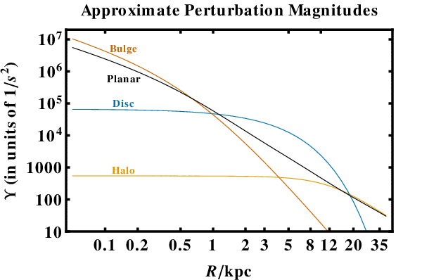
Here, we evaluate the contribution of each component in different regions of the Milky Way. Doing so helps us to understand the dominant effects and to assess the validity of the popular practise of neglecting the planar tides often used in previous works (Heisler & Tremaine, 1986; Matese & Whitman, 1989; Matese & Whitman, 1992; Matese et al., 1995; Breiter et al., 1996; Brasser, 2001; Breiter & Ratajczak, 2005).
We summarize the comparison in Fig. 2. We take and derive the three curves labeled “Bulge”, “Disc” and “Halo” from this partition using Eq. (19) with . The black “Planar” curve is traced from , which represents the amplitude of the right-hand side in Eqs. (15)-(18). The planar perturbations are a function of time, unlike the vertical ones.
Figure 2 shows that the planar contribution to the total tide can reach at least 10% of the total in all regions of the Galaxy, and may reach where the bulge and halo are important. Previous studies’ neglect of the planar tide is then justified at the -level, but only in the regime in which the tidal contribution of the Galactic disc dominates. This regime is typically over Galacotocentric radii between 3.5 and 10 kpc. Therefore, we use this approximation too in Section 4 for our study of the disc regime. Our bulge calculations in Section 5, however, all include the planar tide, in addition to the vertical tide.


Depending on the accuracy sought, only one vertical component of the Milky Way (bulge or disc or halo) needs to be included for many regions of the Galaxy. However, around the bulge-disc transition region, at 1 kpc, and around the disc-halo transition region, at about kpc, two components must be included.
4 The Galactic Disc Regime
4.1 Fiducial Evolution
The range kpc kpc is the most straightforward one in which to explore exoplanet orbital evolution. In this regime, we need to account for only the contribution from the disc () in the vertical tides (see Fig. 2 and Eqs. 20-24). The initial inclination of the planet can also be crucial in determining the effects of the perturbation. The vertical tide vanishes for as is vertically symmetric about the Galactic plane. However, there is little evidence to support coplanarity amongst planetary systems and the Galactic disc.
We then consider a planetary system with – similar to the Solar System – with a one Solar-mass central star. We assume that the star evolves on the main sequence for about 10 Gyr, a value which helps motivate the duration of our numerical simulations. This duration is computationally achievable because our simulations are adiabatic, and often feature wide-orbit single planets.

We provide representative eccentricity evolution profiles for wide-orbit planets residing at different locations in the Galactic disc in Fig. 3. The upper panel demonstrates the dependence on with a fixed value of ; the lower panel illustrates that changing can have a significant effect on the orbital evolution. Over billions of years, bodies at AU orbiting stars within the Solar Circle may become significantly more or less eccentric. The smallest values of typically cause greater perturbations, but not always; exoplanetary systems within the Solar Circle are likely to harbour more dynamically excited scattered discs and Oort clouds than the Solar System. Microlensing observations of wide-orbit eccentric planets residing in the inner parts of the disc represent snapshots of dynamically changing systems.

4.2 Highly-inclined evolution
As the inclination of a planetary system approaches , the variation of the eccentricity is maximized. At , the inclination does not change, and so polar orbits always remain polar orbits. Brasser (2001) found a stationary solution corresponding to ; this value may also be deduced from Eq. (24). The importance of this solution is that, whilst , , and do not change, the eccentricity increases and tends towards unity. Hence, this changing orbit potentially permits collision with the host star or may cause the planet to leave the adiabatic regime.
Although a planet is unlikely to reside in this specific configuration, it is useful to assess how nearby configurations evolve and how the planet’s orbit is affected. We first show that a planet will eventually achieve for all and values in the top two panels of Fig. 4, given and . The resulting survival timescale is higher for tighter planetary orbits and more circular orbits. In the figure, we adopt kpc, approximately halfway between the Earth and the Galactic centre. This choice is motivated by the microlensing planet searches, which are most sensitive to lenses half-way between observer and source star.
Next, we consider small deviations from the stationary orbit. We sample a wide variety of values of , and show in the middle panels of Fig. 4 that for the initial values sampled, at , asymptotically tends towards either or . Doing so eventually causes the eccentricity to tend to unity. Therefore, the value of does not appear to affect the final outcome, just the survival timescale.
By contrast, even if , deviations from will prevent the eccentricity from reaching unity, but still periodically increase its value to nearly unity. The bottom two panels of Fig. 4 illustrate this effect. In those panels, the planets survive even if . However, the eccentricities of those planets achieve values so close to unity that they may become unstable due to other factors, such as close passage to the parent star or a small impulsive kick from other Galactic phenomena. Note importantly from the bottom right panel that even the planet, a full astride from the stationary inclination solution, exhibits eccentricity variations of several tenths. Further, the bottom left panel demonstrates that, although is not stationary, it hovers around , or for the majority of the evolution.
Returning to the strictly stationary orbit, we can estimate the survival timescale, , analytically. By Taylor expanding the inclination about to first order and the eccentricity about to fourth order, we obtain an analytic solution to the first terms of Eqs. (21) and (22). The solution gives, for and respectively,
| (34) |
| (35) |
In both cases, we obtain the same value of the survival timescale when setting , namely
| (36) |
Note that at . We overplot this analytical estimate with large dots on the upper panel of Fig. 4 to demonstrate the quality of the approximation. As expected, the approximation worsens as tends towards unity instead of zero.
Equation (36) suggests that any planet on an adiabatic polar stationary orbit has a finite survival time. For a main sequence lifetime , the critical planetary orbital period around its parent star for which a planet does not survive is
| (37) |
If we apply the disc density law from Eq. (28), then
| (39) | |||||
For a star at kpc, this yields a critical timescale on the order of yr.

5 The Galactic Bulge Regime
Exoplanet evolution in the Galactic bulge regime is more complex due to the importance of both the planar and vertical tides. The vertical tide is composed of the contribution from the bulge, but for locations in the outer bulge (such as at kpc), we must also include the contribution from the disc. Because of the interplay between the vertical and planar tides, attaining compact analytical results is difficult. Hence, we perform numerical simulations to explore phase space.
The results are summarized in Fig. 5. All plots demonstrate a variety of eccentricity profiles; the upper plots model a wide-orbit planet ( AU) and the lower plots illustrate the evolution for a closer-in planet (at AU and AU). All plots assume , except the lower right plot, for which pc and is assumed for all curves. The difference in the evolution profiles from the upper plots (between the kpc and kpc curves) arises from the initial sign of , which is determined by the initial relative magnitudes of Eqs. (21) and (A2).
Wide-orbit planets are significantly affected at all locations in the bulge. In the innermost regions, the timescale of the eccentricity oscillations is fast: on the order of of the typical main sequence lifetime. Also, the evolution in these innermost regions (within a couple hundred parsecs) becomes largely independent of inclination, as shown by the upper right plot. However, other locations in the bulge are affected by changes of inclination. The upper-right panel shows a similar evolutionary pathway to the upper-right panel of Fig. 4, even though here and not .
Tighter-orbit bodies, such as analogues of the trans-Neptunian object Ceto ( AU) and the planet Neptune itself ( AU), are affected significantly only if the host stars reside within the inner hundred parsecs of the bulge. The lower-left plot illustrates the drastic differences in eccentricity profiles due to shifting the value of by just 150 pc. The lower-right plot presents the dependence on for an eccentric Neptune at pc. This planet cannot retain its primordial eccentricity. If, however, the planet was born on a more circular orbit, the extent of the eccentricity change would decrease.
6 Minimum Exoplanet Eccentricity
A planetary system whose invariable plane varies little from the Galactic plane may be modeled in the planar adiabatic limit. Assuming that the planet orbits the star in the same sense that the star orbits the Galactic centre (“prograde”), the equations of motion become:
| (40) | |||||
| (41) | |||||
| (42) | |||||
| (43) |
We plot solutions of these equations in Fig. 6 for planets in the disc at kpc (left panels) and in the bulge at kpc (right panels). We select for all plots except the lower-right plot. The upper panels show that planets in the disc regime typically feature eccentricity variations of to with a period of tens of Myr; planets in the bulge regime show variations of to with a period of a few Myr. These panels illustrate only eccentricity decreases because for each of those curves. We sample at nine equally spaced values from and including and in the lower-left panel, demonstrating the sensitive dependence of the eccentricity evolution on . This dependence is equivalent in the disc and bulge. The lower-right panel instead illustrates the dependence of amplitude on (for ). This relationship between amplitude and is not monotonic because of the term in Eq. (41). Consequently, the greatest variation occurs for .
This term prevents a complete analytical solution to Eqs. (40)-(43). However, under the small eccentricity approximation, one may attain a closed analytical solution for the eccentricity evolution. The solution gives the following maximum eccentricity increase and decrease factors:
| (44) |
where is the planet’s orbital period about its parent star and we used the approximations in Eqs. (32)-(33). Therefore, all exoplanets in the galactic disc have eccentricities which vary by a factor of at least . Note that one cannot use Eq. (44) to determine when a planet will survive because this estimate is based on the adiabatic approximation and for low eccentricity.
Now we consider how Galactic tides affect the pericentre advance or retreat of planets. The maximum variation of is equal to
| (45) |
If we compute the critical semimajor axis at which the maximum pericentre precession rate from Galactic tides is comparable to that from general relativity, we obtain:
| (46) | |||||
where is the speed of light. We emphasize that these precession rate estimates are lower bounds because they were derived in the limiting case of planar adiabatic motion.
7 Discussion
7.1 Implications from Tides
Here, we discuss some of the implications of the tidal results that we have obtained from this work. First, the inclination of the planetary orbit with respect to the Galactic plane might be indicative of dynamical excitation in a planetary system, and vice-versa. Particularly, planetary orbits that are highly inclined to the Galactic plane will feature the greatest excitation. Although survival is likely for the smallest orbits in these systems, their eccentricity variations at a given (fixed) semimajor axis will be higher than in other systems. Despite this variation periodically becoming zero, such periods of dynamical quiescence represent typically just a small fraction of the parent star’s main sequence lifetime. Our lack of unbiased exoplanetary inclination data suggests that we cannot yet pinpoint a preferential planetary inclination with respect to the Galactic disc. However, our own Solar System and the variety of orientations exhibited by transiting planets prove that can easily exist for planetary systems.
Second, our results are not restricted to planets. Our analysis may be extended to binary stars or belts of objects such as Kuiper belts or scattered discs. Jiang & Tremaine (2010) study the evolution of wide binary stars in the Solar neighbourhood. One can instead consider this evolution at other locations in the Galaxy by setting in our Eqs. (12)-(14). For binary stars of equal masses, will be increased by a factor of , and hence, the time evolution of every variable (Eqs. 20-24 and 49-52) will be decreased by a factor of 1.41. The amplitudes of the variations will otherwise remain unaffected. Modeling Kuiper belts and scattered discs involves imposing distributions of initial conditions on our equations. Because the individual bodies in these belts are unlikely to interact with one another, they can be treated by our formalism. Oort clouds are typically too distant to be treated in the adiabatic approximation. Their evolution must be modelled either with N-body simulations (Brasser, 2001; Kaib et al., 2011) or with the nonadiabatic equations of motion (Veras & Evans, 2012).
Third, differential pericentre precession due to Galactic tides might affect long-term N-body simulations of planetary systems. Veras & Ford (2010) highlighted the danger of neglecting general relativity when modeling hierarchical multi-body systems with high relative inclinations, and the effect from Galactic tides might equally be important to incorporate, particularly at high inclinations with respect to the Galactic disc.
Fourth, improving observational precision might be able to place meaningful constraints on planetary systems. Currently, the smallest observational errors on planetary eccentricity measurements are about (Wolszczan, 1994; Welsh et al., 2012). Although these values are well above the baseline eccentricity variations predicted by Eq. (44), and are measured for tight orbits, they might be comparable to expected eccentricity variations for planet WD 0806-661, with AU (Luhman et al., 2011). Two other planets with AU (Goldman et al., 2010; Kuzuhara et al., 2011, e.g.) bolster theories that planets can exist in such remote regions of planetary systems despite being formed elsewhere.
Fifth, the influence of Galactic tides may represent another way in which planets can transform into Hot Jupiters. Near-polar planetary orbits might be highly eccentric (see Fig. 4). The pericentres of these planets might reside close enough to the star such that star-planet tides will damp both the semimajor axis and eccentricity of the planet. The frequency of such transformed Hot Jupiters would be an increasing function of both age and Galactocentric distance. This mechanism is unlikely to be prevalent in the Solar Neighbourhood because the Galactic tidal timescales are likely to be too long to allow for star-planet tides to shrink the planetary orbits appreciably.
7.2 Effects of Passing Stars
Although stars collectively help establish the Galactic tide, individually they can produce strong perturbations when they fly past a planetary system. The consequences of this brief perturbation may be comparable to tides acting over Gyr. The effect of flybys on planetary systems has been studied before in the Galactic Disc (Zakamska & Tremaine, 2004; Veras & Moeckel, 2012, e.g.). Here we quantify the effect in the Galactic bulge.
We use the formalism of Veras & Moeckel (2012), which is sufficiently general to be applied to the bulge. They assumed every star has a single planet on an initially circular orbit, and computed cross sections for the planetary eccentricities to be perturbed by a given amount, . We simplify their treatment by assuming each planet has a mass of and initially resides at the same distance from their parent stars, , all of which are have masses of . Then the number of times, , which a planet’s eccentricity will be changed by over a star’s main sequence lifetime is equal to:
| (47) | |||||
where the normalized cross sections can be read off directly from Figs. 8-11 of Veras & Moeckel (2012), and . We adopt a dispersion velocity of km/s as representative of three-dimensional bulge dispersion velocities. The critical velocity is the encounter velocity at which the total energy of the system is zero and ionization is possible (Fregeau et al., 2004, e.g.):
| (48) |
We consider , AU and compute Gyr by assuming stellar metallicity from Hurley et al. (2000). Figure 7 demonstrates that the minimum possible eccentricity variations due to tides presented in Fig. 6 is likely to be surpassed by passing stars. In the opposite extreme, the eccentricity evolution of planets on wide polar orbits appears to have comparable contributions from tides and stellar flybys (see Fig. 5). Therefore, both of these effects may be equally important and deserve detailed study.

8 Conclusions
The effects of Galactic tides have been studied before in the Solar neighbourhood. This is the first investigation into the effect of tides on planetary systems within the Oort cloud throughout the rest of the disc of our Galaxy, as well as in the bulge.
In the Solar neighbourhood, the Hill surface has an extent of AU. For the Sun, this marks the outer boundary of the Oort Cloud, and Galactic tides are known to play an important role in dislodging comets into the inner Solar System (Smoluchowski & Torbett, 1984; Heisler & Tremaine, 1986; Duncan et al., 1987; Matese & Whitman, 1989; Levison et al., 2001; Kaib & Quinn, 2009). However, the effect of Galactic tides on the Sun’s planets is negligible, even over the age of the Solar system. However, the architecture of exoplanets is very varied, and wide-orbit exoplanets with semimajor axes between 100-2500 AU are known to exist (Kalas et al., 2005; Goldman et al., 2010; Luhman et al., 2011; Kuzuhara et al., 2011, see e.g.,). In the inner Galaxy, the tidal forces are stronger, typically scaling inversely with radius in the Galaxy. For example, in the inner 500 pc, the Hill surface has a size of AU, whilst the timescale over which evolutionary effects become noticeable is billions of years.
The Galactic tide is dominated by the contribution from the Galactic disc over radii in the range 3.5 to 10 kpc. In this disc regime, the popular practice of neglecting the planar tides is justifiable. Planetary systems that are at least moderately inclined to the Galactic disc are susceptible to slow but significant planetary eccentricity evolution over the parent star’s main sequence lifetime. At high inclinations to the Galactic plane, eccentricity evolution is greater. As the semimajor axis is never secularly affected by tidal perturbations, the periastron tends to zero and the planet is driven towards the host star on timescales of yr.
Within 3.5 kpc of the Galactic Centre, the contribution of the Galactic bulge is always important. As the matter distribution is more spherical, the planar tidal components are as important as the vertical ones. Evolution in the bulge regime is now a result of complex interplay between the vertical and planar tides. Wide orbit planets ( AU) are substantially affected by tides on timescales (tens to hundreds of Myr) that are much smaller than the main sequence lifetime ( Gyr). Eccentricity variations of several tenths are very typical for these planets. They are never in a state of quiescence; their orbital parameters are continually changing though the effects of tides. Closer-in planets, at e.g., 100 AU, are only affected if the host star resides within the inner hundred parsecs.
Our study of tides is a first step in the understanding of how exoplanetary systems interact with their Galactic environment. The main limitation of our work is that the host star has been assumed to move in a circular orbit in the Galactic plane. In fact, stars lead much more exciting lives! They are usually inclined to the Galactic plane, their orbits are usually eccentric and sometimes chaotic, and they suffer perturbations that can move them many kiloparsecs. There is, for example, both chemical and dynamical evidence that the Sun has been moved substantially from its place of birth (Clayton, 1997; Sellwood & Binney, 2002) by spiral waves. There are therefore good reasons for believing that the effects of tides are still more substantial than we have found here!
Acknowledgments
We thank an anonymous referee for a helpful and probing report, and Fred C. Adams for reading through the manuscript and providing detailed, useful feedback.
References
- Adams et al. (2006) Adams, F. C., Proszkow, E. M., Fatuzzo, M., & Myers, P. C. 2006, ApJ, 641, 504
- Antonov & Latyshev (1972) Antonov V.A., Latyshev I.N., 1972, in “The Motion and Evolution of Orbits and the Origin of Comets”, IAU Symposium 45, eds Chebotarev A., Kazimirchak-Polonskaia E., Marsden B.G., Reidel, Dordrecht, p. 341
- Batalha et al. (2012) Batalha, N. M., Rowe, J. F., Bryson, S. T., et al. 2012, arXiv:1202.5852
- Bate (2012) Bate, M. R. 2012, MNRAS, 419, 3115
- Batista et al. (2009) Batista, V., Dong, S., Gould, A., et al. 2009, A&A, 508, 467
- Bennett et al. (2006) Bennett, D. P., Anderson, J., Bond, I. A., Udalski, A., & Gould, A. 2006, ApJL, 647, L171
- Binney & Tremaine (1987) Binney, J., & Tremaine, S.. 1987, Galactic Dynamics, Princeton University Press, Princeton
- Binney & Merrifield (1998) Binney, J., & Merrifield, M. 1998, Galactic Astronomy, Princeton University Press, Princeton
- Boley (2009) Boley, A. C. 2009, ApJL, 695, L53
- Boley et al. (2012) Boley, A. C., Payne, M. J., & Ford, E. B. 2012, ApJ, 754, 57
- Borucki et al. (2011a) Borucki, W. J., Koch, D. G., Basri, G., et al. 2011a, ApJ, 728, 117
- Borucki et al. (2011b) Borucki, W. J., Koch, D. G., Basri, G., et al. 2011b, ApJ, 736, 19
- Boss (1997) Boss, A. P. 1997, Science, 276, 1836
- Boss (2003) Boss, A. P. 2003, ApJ, 599, 577
- Boss (2006) Boss, A. P. 2006, ApJL, 637, L137
- Boss (2011) Boss, A. P. 2011, ApJ, 731, 74
- Brasser (2001) Brasser, R. 2001, MNRAS, 324, 1109
- Brasser et al. (2010) Brasser, R., Higuchi, A., & Kaib, N. 2010, A&A, 516, A72
- Breiter et al. (1996) Breiter, S., Dybczynski, P. A., & Elipe, A. 1996, A&A, 315, 618
- Breiter & Ratajczak (2005) Breiter, S., & Ratajczak, R. 2005, MNRAS, 364, 1222
- Burns (1976) Burns, J. A. 1976, American Journal of Physics, 44, 944
- Cameron (1978) Cameron, A. G. W. 1978, Moon and Planets, 18, 5
- Cassan et al. (2012) Cassan, A., Kubas, D., Beaulieu, J.-P., et al. 2012, Nature, 481, 167
- Clayton (1997) Clayton D., 1997, ApJL, 484, L67
- Deleuil et al. (2008) Deleuil, M., Deeg, H. J., Alonso, R., et al. 2008, A&A, 491, 889
- Dodson-Robinson et al. (2009) Dodson-Robinson, S. E., Veras, D., Ford, E. B., & Beichman, C. A. 2009, ApJ, 707, 79
- Dong et al. (2009) Dong, S., Bond, I. A., Gould, A., et al. 2009, ApJ, 698, 1826
- Duncan et al. (1987) Duncan, M., Quinn, T., & Tremaine, S. 1987, AJ, 94, 1330
- Dwek et al. (1995) Dwek, E., Arendt, R. G., Hauser, M. G., et al. 1995, ApJ, 445, 716
- Duncan et al. (1987) Duncan, M., Quinn, T., & Tremaine, S. 1987, AJ, 94, 1330
- Evans & de Zeeuw (1992) Evans N.W,, de Zeeuw P.T. 1992, MNRAS, 257, 152
- Evans (1993) Evans N.W., 1993, MNRAS, 260, 191
- Feast & Whitelock (1997) Feast M., Whitelock P., 1997, MNRAS 291, 683
- Fellhauer et al. (2006) Fellhauer M., et al. 2006, ApJ, 651, 167
- Flynn & Fuchs (1994) Flynn C., Fuchs B., 1994, MNRAS, 270, 471
- Fouchard (2004) Fouchard, M. 2004, MNRAS, 349, 347
- Fouchard et al. (2006) Fouchard, M., Froeschlé, C., Valsecchi, G., & Rickman, H. 2006, Celestial Mechanics and Dynamical Astronomy, 95, 299
- Fregeau et al. (2004) Fregeau, J. M., Cheung, P., Portegies Zwart, S. F., & Rasio, F. A. 2004, MNRAS, 352, 1
- Goldman et al. (2010) Goldman, B., Marsat, S., Henning, T., Clemens, C., & Greiner, J. 2010, MNRAS, 405, 1140
- Grether & Lineweaver (2006) Grether, D., & Lineweaver, C. H. 2006, ApJ, 640, 1051
- Heisler & Tremaine (1986) Heisler, J., & Tremaine, S. 1986, Icarus, 65, 13
- Huang & Wade (1966) Huang, S.-S., & Wade, C., Jr. 1966, ApJ, 143, 146
- Hurley et al. (2000) Hurley, J. R., Pols, O. R., & Tout, C. A. 2000, MNRAS, 315, 543
- Janczak et al. (2010) Janczak, J., Fukui, A., Dong, S., et al. 2010, ApJ, 711, 731
- Jiang & Tremaine (2010) Jiang, Y.-F., & Tremaine, S. 2010, MNRAS, 401, 977
- Kaib & Quinn (2009) Kaib, N. A., & Quinn, T. 2009, Science, 325, 1234
- Kaib et al. (2011) Kaib, N. A., Roškar, R., & Quinn, T. 2011, Icarus, 215, 491
- Kalas et al. (2005) Kalas, P., Graham, J. R., & Clampin, M. 2005, Nature, 435, 1067
- Kuzuhara et al. (2011) Kuzuhara, M., Tamura, M., Ishii, M., Kudo, T., Nishiyama, S., & Kandori, R. 2011, AJ, 141, 119
- Levison et al. (2001) Levison, H. F., Dones, L., & Duncan, M. J. 2001, AJ, 121, 2253
- Levison & Stewart (2001) Levison, H. F., & Stewart, G. R. 2001, Icarus, 153, 224
- Lin & Ida (1997) Lin, D. N. C., & Ida, S. 1997, ApJ, 477, 781
- Luhman et al. (2011) Luhman, K. L., Burgasser, A. J., & Bochanski, J. J. 2011, ApJL, 730, L9
- Luhman et al. (2012) Luhman, K. L., Burgasser, A. J., Labbé, I., et al. 2012, ApJ, 744, 135
- Malmberg et al. (2011) Malmberg, D., Davies, M. B., & Heggie, D. C. 2011, MNRAS, 411, 859
- Marcy & Butler (2000) Marcy, G. W., & Butler, R. P. 2000, PASP, 112, 137
- Matese & Whitman (1989) Matese, J. J., & Whitman, P. G. 1989, Icarus, 82, 389
- Matese & Whitman (1992) Matese, J. J., & Whitman, P. G. 1992, Celestial Mechanics and Dynamical Astronomy, 54, 13
- Matese et al. (1995) Matese, J. J., Whitman, P. G., Innanen, K. A., & Valtonen, M. J. 1995, Icarus, 116, 255
- Matese & Whitmire (1996) Matese, J. J., & Whitmire, D. 1996, ApJL, 472, L41
- Miyake et al. (2011) Miyake, N., Sumi, T., Dong, S., et al. 2011, ApJ, 728, 120
- Moeckel et al. (2012) Moeckel, N., Holland, C., Clarke, C. J., & Bonnell, I. A. 2012, MNRAS, 425, 450
- Murray & Dermott (1999) Murray, C. D., & Dermott, S. F. 1999, Solar System Dynamics, Cambridge University Press, Cambridge
- Parker & Quanz (2012) Parker, R. J., & Quanz, S. P. 2012, MNRAS, 419, 2448
- Perets & Kouwenhoven (2012) Perets, H. B., & Kouwenhoven, M. B. N. 2012, ApJ, 750, 83
- Pinfield et al. (2012) Pinfield, D. J., Burningham, B., Lodieu, N., et al. 2012, MNRAS, 422, 1922
- Pollack et al. (1996) Pollack, J. B., Hubickyj, O., Bodenheimer, P., et al. 1996, Icarus, 124, 62
- Rasio & Ford (1996) Rasio, F. A., & Ford, E. B. 1996, Science, 274, 954
- Raymond & Armitage (2012) Raymond, S. N., & Armitage, P. J. 2012, arXiv:1211.2809
- Sahu et al. (2006) Sahu, K.C., et al. 2006, Nat, 443, 534
- Scharf & Menou (2009) Scharf, C., & Menou, K. 2009, ApJL, 693, L113
- Sellwood & Binney (2002) Sellwood J., Binney J.J. 2002, MNRAS, 336, 785
- Smoluchowski & Torbett (1984) Smoluchowski, R., & Torbett, M. 1984, Nature, 311, 38
- Spiegel et al. (2011) Spiegel, D. S., Burrows, A., & Milsom, J. A. 2011, ApJ, 727, 57
- Sterzik & Durisen (1995) Sterzik, M. F., & Durisen, R. H. 1995, A&A, 304, L9
- Sumi et al. (2011) Sumi, T., Kamiya, K., Bennett, D. P., et al. 2011, Nature, 473, 349
- Thommes et al. (2002) Thommes, E. W., Duncan, M. J., & Levison, H. F. 2002, AJ, 123, 2862
- Varvoglis et al. (2012) Varvoglis, H., Sgardeli, V., & Tsiganis, K. 2012, Celestial Mechanics and Dynamical Astronomy, 113, 387
- Veras et al. (2009) Veras, D., Crepp, J. R., & Ford, E. B. 2009, ApJ, 696, 1600
- Veras & Evans (2012) Veras, D., & Evans, N. W. 2012, Celestial Mechanics & Dynamical Astronomy, in press, arXiv:1210.6658
- Veras & Ford (2010) Veras, D., & Ford, E. B. 2010, ApJ, 715, 803
- Veras & Moeckel (2012) Veras, D., & Moeckel, N. 2012, MNRAS, 425, 680
- Weidenschilling & Marzari (1996) Weidenschilling, S. J., & Marzari, F. 1996, Nature, 384, 619
- Welsh et al. (2012) Welsh, W. F., Orosz, J. A., Carter, J. A., et al. 2012, Nature, 481, 475
- Wilkinson & Evans (1999) Wilkinson, M. I., Evans, N. W., 1999, MNRAS, 310, 645
- Wolszczan (1994) Wolszczan, A. 1994, Science, 264, 538
- Yee et al. (2012) Yee, J. C., Shvartzvald, Y., Gal-Yam, A., et al. 2012, arXiv:1201.1002
- Zakamska & Tremaine (2004) Zakamska, N. L., & Tremaine, S. 2004, AJ, 128, 869
Appendix A Planar Adiabatic Equations
We obtain the planar adiabatic equations for a planet subjected to tidal perturbations by setting in Eqs. (25)-(29) of Veras & Evans (2012):
| (49) | |||||
| (50) | |||||
| (51) | |||||
| (52) | |||||
| (53) |
where, using the notation of Veras & Evans (2012), we have
| (54) | |||||
| (55) | |||||
| (56) | |||||
| (57) |