Three-body calculation of the rate of reaction in the Sun
Abstract
Using expansion of the three-body wave function of the system in the initial state on hyperharmonic functions, the rate of the reaction in the Sun is calculated. The results of calculation of the flux at 1 AU are compared with the results of a measurement made by the Borexino collaboration and Bahcall et al. theoretical predictions.
pacs
21.45.-v, 23.40.Bw, 26.65.+t, 27.10.+hI Introduction
The study of the neutrino from the Sun is a multipurpose problem. Indeed, the measurement of the solar neutrino flux incident on the Earth helps to clarify the properties of the neutrino; for example, the phenomenon of the oscillations and to determine its parameters (the mixing angle and the eigenmass of the neutrino). Then, the value of the flux and its spectral properties contain in some cases information on the nuclear reactions that in the visible future cannot be observed in the laboratory. We mean here the reactions:
| (1) |
and
| (2) |
Moreover, as emphasized by John N. Bahcall in his book and in a series of papers [1, 2, 3, 4, 5] (see also [6]), solar neutrinos bring the information about processes in the center of star connected with solar structure models.
Although the reaction (2), called the reaction, plays no significant role in hydrogen burning of stars, it is essential in detecting monoenergetic neutrinos of MeV. Also, a measurement of the neutrino flux from reaction (2) can be useful for the determination of the parameters of the Standard Solar Model.
All the above considerations contain sets of parameters used for fitting observable data in the framework of different models such as star models, nuclear reactions models, and so on. An example of such a type is the two-body model [7] for reaction (2) which is essentially three body [8].
The purpose of this work is to exclude the model elements as much as possible in the description of reaction (2) and to treat the initial state as a purely three-body state. From a strict point of view, the modern treatment of any nuclear reaction inside the Debye-sphere is still the model in a sense of the absence of the dynamical consideration (it is the six-body problem in the Sun’s interior condition) of particles inside the sphere. We hope, however, that the three-body instead of the two-body treatment of reaction (2) is a step in the right direction.
Below, we concentrate ourselves mainly on the process (2) for the following reasons. First, in 2012 the results of the first experimental observation of process (2) was announced [9], after more than 50 years of studies of solar neutrino problems. The second reason is connected with the absence of a three-body treatment of the initial state in process (2).
There is a question concerning sensitivity to the choice of the nucleon-nucleon potential and related to these potentials wave functions of the bound state of the deuteron and the continuum state of the system.
With all this in mind we present below the treatment which takes into account all peculiarities of the three-body system. In Sec. II we start from the inputs for the problem considered: the weak Hamiltonian and -potentials, then in Sec. III, we consider the solution of the Schrödinger equation to determine the wave function of the initial state. In Sec. IV, we present the calculation of the probability of the reaction and the astrophysical factor taking into account the Coulomb and strong interactions simultaneously. The results for the rate of the process and fluxes of the neutrino are discussed in Section V and conclusions are presented in Section VI. The relevant Schrödinger equation for the three interacting particles along with its hyperharmonics method of solution is shown in Appendix A. We have used the program MATHEMATICA (version 7) for our calculations.
II Inputs
The electron capture by the nuclear system can be described by the following nonrelativistic effective weak Hamiltonian [10]
| (3) |
where ( is the neutrino momentum); ,, and are the matrix unit operators and spin angular momentum operators for the lepton and ith nucleon; and are the space coordinates of the lepton and an ith nucleon; are the isobaric-spin operators which transfom a lepton electron state into a lepton neutrino state and ith nucleon proton state into an ith nucleon neutron state; and , and are the vector, axial vector and “induced” pseudoscalar coupling constants, respectively. We take and [11]. We can simplify the weak Hamiltonian for the system: the last term in Eq. (3) can be neglected because the emitted neutrino has energy MeV and this term encloses factor , where is the proton mass; the transition satisfies the Gamow-Teller selection rule; therefore, the first term of Eq. (3) does not give contribution to the matrix element of transition. Finally we take into account that the electron neutrino has spin opposite to its momentum . Finally, for the weak Hamiltonian we get
| (4) |
With this Hamiltonian of Eq. (4) we obtain the electron capture transition matrix element.
The energy of thermalization of particles in the interior of the Sun corresponds to keV which is small on the nuclear energy scale. Therefore, we can use the simple -potential which describes correctly the low energy data of the nucleon-nucleon system. We apply the Gauss and the Yukawa potentials [12]. We fit the parameters of these potentials to get the values of the deuteron energy, the scattering lengths and the effective ranges for and scattering.
For the Gauss potential
| (5) |
the calculation with the fitted parameters
gives the scattering length fm and the effective range fm for scattering at the singlet state , while the parameters
lead to the scattering length fm, the effective range fm for scattering at the triplet state and the binding deuteron energy MeV.
The second potential is the Yukawa potential
| (6) |
with the parameters for the singlet state:
and for the triplet state:
The results of calculation of the scattering lengths and effective ranges are:
| (7) |
To find the neutrino flux we must use some Standard Solar Model (SSM). There are several SSMs which are in good agreement with the helioseismologically determined sound speed, temperature and density of elements as a function of solar radius, the depth of the convective zone, the surface helium abundance, and so on. We applied data of parameters presented in the model BS05(OP) [13]. The results of Bahcall et al. [4] shows that the flux from the reaction is not sensitive to the type of SSM.
III The wave function of the initial state
We note that Bahcall and May [7] used the wave function in a factorized form as the product of the wave function of the relative motion of two protons and the wave function of the electron moving in the Coulomb field of these protons. However, such a representation is not quite a correct procedure due to the long-range nature of the Coulomb interaction, even for the asymptotic behavior of the wave function when electron is at a large distance from the protons [14, 15]. All the more, we cannot perform such a factorization at a small relative distance where we need to know the wave function with a sufficient accuracy to get a good accuracy of the calculation for the transition matrix element of the process . Also, there is a problem with the total angular momentum of , because the moments of subsystems are not conserved. Fortunately, the relative angular moment of two nucleons in the initial and final states is zero as angular moments of the electron and the neutrino; therefore, the last problem did not arise in the Bahcall calculations of the reaction.
We use the hyperspherical harmonics [16, 17] for expansion of the wave function in the initial state and solve directly the three-body Schrödinger equation and, therefore, we are free of the problems which we mentioned above. As in the nonrelativistic approach the orbital and spin moments are conserved independently of one another, we can expand the spatial part of the three-particle wave function over hyperspherical functions and we obtain the linked system of the radial differential equations. Derivation of the system radial equations is given in Appendix A. To proceed further, we now use the system of Eqs. (60) for the radial wave functions. Since the total energy of the system is low, the main contribution to the three-particle wave function gives the states with the zero relative orbital moments. Owing to the centrifugal potential and at small distance where we need to calculate the wave function with higher accuracy, contributions of the components with the hypermoments should be suppressed in the total wave function. Taking into account these conditions, we need to find the solution of the single equation only for and with the nondiagonal terms omitted. We omit all the indices because they correspond to zero values of the quantum numbers and get the equation for the radial wave function :
| (8) |
where ( is the total energy of the system);
| (9) | |||||
| (10) |
Here is the three-body Coulomb parameter which is defined as
| (11) | |||||
| (12) | |||||
| (13) | |||||
| (14) |
The matrix element of the nuclear potential is the following: for the Gauss potential
| (15) |
and for the Yukawa potential
| (16) |
where is the modified Bessel function of the first kind, and is the modified Struve function.
To find a unique solution of Eq. (8) for the continuous state of the system, we must determine boundary conditions. Instead of defining the function and its derivative at the origin (), we define the wave function at a point close to zero because we know the behavior of the wave function near the origin. At small distances from the origin they have a form 11 1 We take the point not equal to zero for reasons of the numerical calculations..
| (17) |
where .
The wave function at large distance, where the nuclear interaction is negligible, has the following asymptotics:
| (18) |
where is the three-body nuclear scattering phase shift modified by the Coulomb interactions, and are the three-body regular and irregular Coulomb wave functions, respectively, and are defined as
| (19) | |||||
| (20) | |||||
where is the three-body Coulomb phase shift given by
| (21) |
and is the Whittaker function. In the numerical calculations, when we are dealing with large values of the Coulomb parameter and , it is best to use another representation of the function :
| (22) | |||||
where is the confluent hypergeometric function.
We solve Eq. (8) using the boundary conditions (17) and then matching the logarithmic derivative of the solution in the asymptotic region with the logarithmic derivative of the asymptotic solution [Eq. (18)] we define the three-body phase shift which depends on the total energy of the system. The numerical calculations with the Gauss potential yield the following values of the phase shifts: at the energy keV corresponding to the temperature at the core of the Sun, we obtain radian, while at keV it is radian. Even with energy as high as 20 keV, the values of the phase shift remains very small. We get the same results with the Yukawa potential.
Matching the numerically obtained solution of the Schrödinger equation with its asymptotics allows us also to find the normalization factor. At large distances the ratio of the unnormalized solution to the asymptotic function becomes a constant.
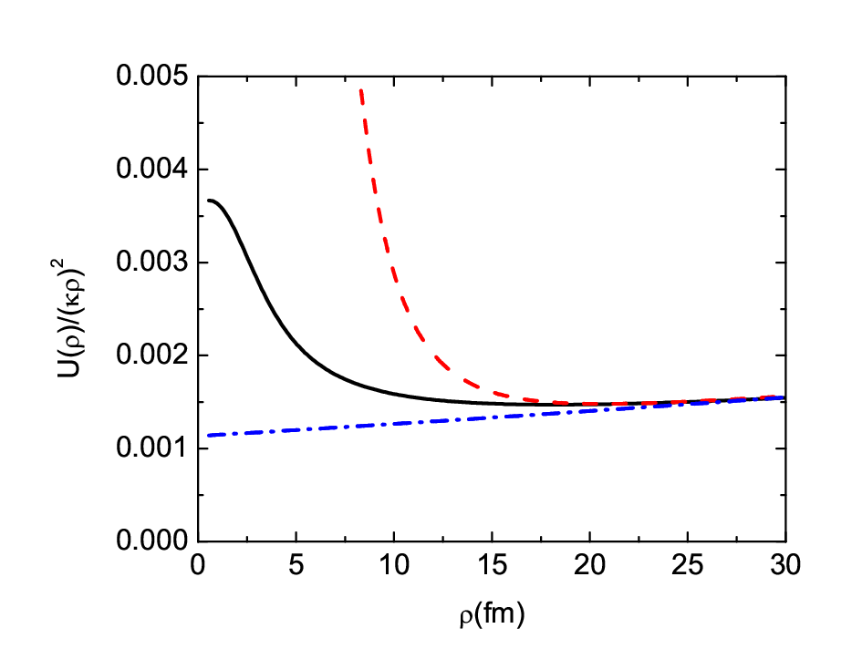
Figure 1 shows the results of calculation of the radial wave function (solid curve) at keV and its asymptotics (18) for the Gauss potential (dashed curve). Since the scattering phase shift is close to zero at the considered energy range the pure three-body Coulomb wave (dot-dashed curve) is close to the solution of the Schrödinger equation at the distances fm. Note that all functions presented on Figure 1 are divided by . As seen in Figure 1, the function has a linear dependence on at the considered range of the variable . We obtain the same results for the Yukawa potential.
We need to know the three-body wave function with high accuracy in the interval fm because the deuteron wave function cuts integration at the distance 35 fm when we calculate the matrix element of the transition.
IV The probability of the reaction and astrophysical factor
Using the weak Hamiltonian (Eq. (4)) we can write the matrix element of the reaction as
| (23) | |||||
where and are the spin functions of the electron and neutrino, respectively; is the wave function of the deuteron, while is the three-body wave function of the system in a continuous state. The neutrino wave function can be taken as a plane wave, because it does not interact with the deuteron. At the energy of the emitted neutrino is 1.44 MeV and the de Broglie wavelength of the neutrino is almost 900 fm, implying the plane wave is essentially unity over the effective volume of the deuteron (the difference from unity is about 0.2%). Accordingly, we take . In the wave function the electron coordinate is taken at the point where one of the protons is placed.
Since the weak interaction is small, first-order perturbation theory can be applied to calculate of the probability of reaction per unit of time; therefore, we have
| (24) |
where the overline means summation over spins in the final state and averaging over spins in the initial state, and the density of neutrino states is
| (25) |
Here , and are the neutrino energy and light speed, respectively. Using the energy conservation law we define
where is the kinetic energy of proton-proton relative motion, are the deuteron, proton and electron masses, respectively. If we put kinetic energies of the particles to zero, we get MeV.
Averaging in Eq. (24) and using the Jacobi coordinates for the particles defined by Eq. (51) of Appendix A we obtain
| (26) |
Note that the presence of the delta-function in the weak Hamiltonian (4) leads to calculation of the integral over the variable to the value of the wave function at the distance .
The deuteron wave function can be written in the form
| (27) |
where the radial wave function is normalized so that the deutron wave function is normalized to unity.
Using the first term of Eq. (59) from Appendix A and taking into account that the three-body wave function of the system in the initial state can be written as
| (28) |
Taking into account the last two equations, we obtain that the overlap integral is
| (29) |
Here the three-body radial wave function is calculated at the point .
Usually in the nuclear astrophysics, for parameterizations of a two-body reaction cross section the astrophysical factor is used [18]. To find the factor from the cross section, the Gamow factor is extracted from the cross section, i.e.
| (30) |
where is the Sommerfeld (Coulomb) factor for the colliding nuclei with charges and having the relative velocity . A similar procedure can be carried out for the reaction with three particles in the initial state because the three-body radial wave function of the continuum state at a distance larger than the nuclear interaction radius encloses factor . Therefore we define the astrophysical factor for the reaction as
| (31) | |||||
| (32) |
is almost a linearly varying function of and is not equal to zero, like the astrophysical factor for two-body reactions. Note that the unit of coincides with the unit of because is dimensionless and it is the Gamow factor for the reaction. If we use expansion of over as
| (33) |
we obtain the following results for the value of the
coefficients:
For the Gauss potentials
| (34) |
and for the Yukawa potentials
| (35) |
Behavior of the astrophysical factor on energy is presented in Fig. 2 where linear dependence of the factor is seen clearly for both potentials. The small difference between the factors for the Gauss and Yukawa potentials can be explained by small differences of the obtained low energy scattering parameters.

To check the validity of the results of our calculations of the reaction, we calculated the astrophysical factor for the reaction, according to the conventional definition (Eq. (30)) by the same potentials. If is approximated by a polynomial
| (36) |
we get the following results:
For the Gauss potentials
| (37) |
and for the Yukawa potentials
| (38) |
These results are very close to data presented in [18].
V Rate of the reaction and the solar neutrino flux
We introduce the rate constant of the reaction as
| (39) |
where is the Maxwell-Boltzmann distribution function for particles of mass and velocity and is the Boltzmann constant. Excluding the velocity of the center of mass of the system and taking into account the fact that the center of mass of the system is almost the same as the center of the system we get
| (40) |
where , is the relative velocity of protons and . Taking into account that
and making transformations
we obtain
| (41) |
Using Eqs. (31), (32) we finally obtain
| (42) |
We note that the rate constant depends on the temperature and the nature of the reactants, but does not depend on their concentration. If we define the Gamow energy as
| (43) |
the integrand of Eq. (42) is a maximum at the energy
| (44) |
Here is defined through Eqs. (12), (13) and (14) and it equals to
| (45) |
Note that, if we take we obtain the point of maximum of the integrand in the equation of the reaction rate constant.
To obtain the rate of reactions, the rate constant must be multiplied by the density of the reactants,
| (46) |
where and are the numbers of electrons and protons in the unit of volume.
All solar parameters like temperature and densities of protons and electrons vary with the radius of the interior of the Sun. The results for the neutrino fluxes presented by Bahcall et al. [5] show that the fluxes from the and reaction are not sensitive to the considered solar models. Therefore, to calculate of the rates of the and reaction we apply the BS05(OP) model [6].
Figure 3 shows the rate of the and reaction as a function or the solar interior radius for the Gauss potentials. We obtain the same behavior in the case of the Yukawa potentials. We see that the rate of the reactions is more than a hundred times less than the rate of the reaction for the whole distance from the center of the Sun, and reactions occur in the core of the Sun where the temperature and density are higher.

Integrating the reaction rate (46) over the volume of the Sun we find the total flux of neutrinos emitted by the Sun. Dividing this total flux by the area of the sphere of the radius of one astronomical unit (AU) we obtain the neutrino flux passing through a unit area of the Earth surface. The results of calculations of the neutrino fluxes are presented in Table 1.
| Standard Solar | References | |||
| Model | ||||
| BS05(OP) | 6.20 | 2.04 | 304 | our results |
| with Gauss | ||||
| potential | ||||
| BS05(OP) | 6.05 | 1.99 | 304 | our results |
| with Yukawa | ||||
| potential | ||||
| BP04(Yale) | 5.94 | 1.40 | 424 | [4] |
| BP04(Garching) | 5.94 | 1.41 | 421 | [4] |
| BS04 | 5.94 | 1.40 | 424 | [4] |
| BS05(14N) | 5.99 | 1.42 | 421 | [4] |
| BS05(OP) | 5.99 | 1.42 | 421 | [4] |
| BS05(AGS,OP) | 6.06 | 1.45 | 418 | [4] |
| BS05(AGS,OPAL) | 6.05 | 1.45 | 417 | [4] |
Note that the results for the neutrino flux from the reaction are close to the results obtained by Bahcall et al. while there are differences between the fluxes from the reactions.
The Borexino collaboration announced the results of the neutrino flux measurement: [9]. Taking into account that the survival probability of the neutrino (due to the neutrino oscillation) in the reaction predicted by the Borexino collaboration equals at 1.44 MeV [9], we find that the neutrino flux at 1 AU should be equal to for the Gauss potential, and for the Yukawa potential.
We note that our results for the neutrino fluxes from the reaction obtained by taking into account the survival probability lie within the confidence interval of the experimental data. At the same time, the Bahcall results are out of this limit at all fluxes listed in Table 1 if they are multiplied by the same survival probability of the neutrino. Comparing our calculated low-energy parameters for the Gauss and Yukawa potentials, we see that they differ by 2% to7%, and the neutrino fluxes from the have a 2% difference, too, and the results of of Bahchall et al. shown in Table 1 for all SSMs are not more than 2% to 4% from our calculated . Therefore, we may conclude that the dependence of the results on the type of potentials is very weak. However, the difference in the results obtained by ourselves and Bahcall et al. can reach up to 39% to 45%, which means strong sensitivity to the choice of the wave functions of the initial three-body state of the system.
VI Conclusion
In the framework of the three-body approach the probability of the process under conditions of the solar core has been found. The rate of the above process and neutrino flux are found and compared with the Borexino experiment and previous calculations. The value of the neutrino flux obtained from the reaction in the three-body treatment appeared to be % larger as compared to the Bahcall et al. value. This can be understood as a correct description of the movement of the electron producing the screening effect between protons. In this work we have introduced the astrophysical factor for the three-body reaction which is an analog of the factor introduced for binary processes. To discriminate between different star models on the basis of our results, it is necessary to essentially reduce experimental errors in the above experiment.
Acknowledgments
The authors are very grateful to Prof. O. A. Zaimidoroga for fruitful discussions and useful comments.
Appendix A Schrödinger equation
The Hamiltonian of the system is
| (47) |
where is kinetic energy operator:
| (48) |
subscript means electron, while and correspond to two protons; is the reduced mass of two protons, while is the reduced mass of the system of two protons and electron;
| (49) |
is the sum of the Coulomb potentials in the system, and is the nuclear potential of interaction between two nucleons.
The wave function of the initial state of the system is the eigenfunction of the Hamiltonian (47), which has a continuous spectrum of energy and satisfies the Schrödinger equation
| (50) |
Let us define the Jacobi coordinates:
| (51) | |||||
where is the reduced mass of two protons, indices i j k=123, 231, or 312 and () is the mass (coordinate) of particle . In introducing coordinates the Hamiltonian of the free motion of particles can be written as
| (52) | |||||
We define the square of the hyperradius and hyperangle as:
In the variables of hyperradius and a set of angles ( and are unit vectors determining the azimuthal and polar angles)), we can rewrite the operator as
| (53) |
where the operator is
| (54) | |||||
where is an angular part of the Laplace operator.
The hyperspherical function is defined as the solution of the equation [16]
| (55) |
The quantum number is called hypermoment, the eigenfunction is
| (56) |
where the function is
| (57) |
is the Clebsch-Gordon coefficient; is the spherical function;
| (58) |
must be an integer number; is Jacobi polynomial.
Let and be conjugate momenta to the coordinates and . Then determining square of the wave number ( is the total energy of the system in the c.m. frame) for the system in the continuous state, removing a free motion of the center of mass of the system from Eq. (50) and using the following expansion of the wave function of a continuous spectrum over the hyperharmonics functions
| (59) |
we get the radial Schrödinger equation:
| (60) |
where superscript denotes taking complex conjugate of the function, and , where is defined on a hypersphere of unit radius in a six dimensional momentum space. The matrix element equals to
| (61) | |||
The system of Eq. (60) is a system of the linked one dimensional equations which must satisfy the boundary conditions depending on the particular physical situation.
References
- [1] J. N. Bahcall, Neutrino Astrophysics, (Cambridge University Press, Cambridge) 1989.
- [2] J. N. Bahcall, Nucl. Phys. Proc. Suppl. 118, 77 (2003).
- [3] J. N. Bahcall, and M. H. Pinsonneault, Phys. Rev. Lett. 92, 121301 (2004).
- [4] J. N. Bahcall, A. M. Serenelli, and S. Basu, ApJ 621, L85 (2005); arXiv:astro-ph/0412440.
- [5] J. N. Bahcall, A. M. Serenelli, and S. Basu, ApJ Suppl. 165, 400 (2006).
- [6] http://www.sns.ias.edu/jnb/
- [7] J. N. Bahcall and R. M. May, ApJ 155, 501 (1969).
- [8] V. B. Belyaev, S. V. Levin, S. L. Yakovlev, J. Phys. B37, 1369 (2004).
- [9] G. Bellini et al. (Borexino Collaboration), Phys. Rev. Lett. 108, 051302 (2012).
- [10] H. Primakoff, Rev. Mod. Phys. 31, 802 (1959).
- [11] B. Povh, K. Rith, C. Scholz, F. Zetsche, Particles and Nuclei: An Introduction to the Physical Concepts, 6th ed. (Springer-Verlag, Berlin, Heidelberg, 2008).
- [12] J. M. Blatt, V. F. Weisskopf, Theoretical nuclear physics, New York: Springer-Verlag, 1979.
- [13] http://www.sns.ias.edu/jnb/SNdata/Export/BS2005/ bs05op.dat.
- [14] E. O. Alt and A. M. Mukhamedzhanov, Phys. Rev. A 47, 2004 (1993).
- [15] A. M. Mukhamedzhanov and M. Lieber, Phys. Rev. A 54, 3078 (1996).
- [16] R. I. Djibuti and K. V. Shitikova, Metod hipersfericheskih funktsiy v atomnoy i yadernoy fizike (Method of hyperspherical functions in atomic and nuclear physics), (Energoatomizdat,Moscow, 1993),in Russian.
- [17] M. Fabre de la Ripelle, S. A. Sofianos, R. M. Adam, Annals of Physics 316, 107 (2005).
- [18] C. Angulo et al., Nucl. Phys. A 656, 3 (1999).