跳到论文正文
W Papers独立论文阅读器 arXiv:1212.3850 论文正文 计算阅读时间 · 0%
引用这篇论文根据当前论文元数据生成,正式投稿前建议核对。


License: arXiv.org perpetual non-exclusive license
arXiv:1212.3850v1 [cs.IT] 16 Dec 2012

Belief Propagation for Continuous State Spaces:
Stochastic Message-Passing with Quantitative Guarantees

Nima Noorshams1 Martin J. Wainwright1,2
nshams@eecs.berkeley.edu wainwrig@eecs.berkeley.edu

Department of Statistics2 and

Department of Electrical Engineering &\& Computer Science1

University of California Berkeley

December 2012

Keywords: Graphical models; sum-product algorithm for continuous state spaces; low-complexity belief propagation; stochastic algorithm; orthogonal basis expansion.

Abstract

The sum-product or belief propagation (BP) algorithm is a widely used message-passing technique for computing approximate marginals in graphical models. We introduce a new technique, called stochastic orthogonal series message-passing (SOSMP), for computing the BP fixed point in models with continuous random variables. It is based on a deterministic approximation of the messages via orthogonal series expansion, and a stochastic approximation via Monte Carlo estimates of the integral updates of the basis coefficients. We prove that the SOSMP iterates converge to a δ\delta-neighborhood of the unique BP fixed point for any tree-structured graph, and for any graphs with cycles in which the BP updates satisfy a contractivity condition. In addition, we demonstrate how to choose the number of basis coefficients as a function of the desired approximation accuracy δ\delta and smoothness of the compatiblity functions. We illustrate our theory with both simulated examples and in application to optical flow estimation.

1 Introduction

Graphical models provide a parsimonious yet flexible framework for describing probabilistic dependencies among large numbers of random variables. They have proven useful in a variety of application domains, including computational biology, computer vision and image processing, data compression, and natural language processing, among others. In all of these applications, a central computational challenge is the marginalization problem, by which we mean the problem of computing marginal distributions over some subset of the variables. Naively approached, such marginalization problems become intractable for all but toy problems, since they entail performing summation or integration over high-dimensional spaces. The sum-product algorithm, also known as belief propagation (BP), is a form of dynamic programming that can be used to compute exact marginals much more efficiently for graphical models without cycles, known as trees. It is an iterative algorithm in which nodes in the graph perform a local summation/integration operation, and then relay results to their neighbors in the form of messages. Although it is guaranteed to be exact on trees, it is also commonly applied to graphs with cycles, in which context it is often known as loopy BP. For more details on graphical models and belief propagation, we refer the readers to the papers [14, 27, 2, 15, 28].

In many applications of graphical models, we encounter random variables that take on continuous values (as opposed to discrete). For instance, in computer vision, the problem of optical flow calculation is most readily formulated in terms of estimating a vector field in ℝ2\mathbb{R}^{2}. Other applications involving continuous random variables include tracking problems in sensor networks, vehicle localization, image geotagging, and protein folding in computational biology. With certain exceptions (such as multivariate Gaussian problems), the marginalization problem is very challenging for continuous random variables: in particular, the messages correspond to functions, so that they are expensive to compute and transmit, in which case belief propagation may be limited to small-scale problems. Motivated by this challenge, researchers have proposed different techniques to reduce complexity of BP in different applications [3, 25, 8, 12, 7, 13, 23, 19]. For instance, various types of quantization schemes [7, 13] have used to reduce the effective state space and consequently the complexity. In another line of work, researchers have proposed stochastic methods inspired by particle filtering [3, 25, 8, 12]. These techniques are typically based on approximating the messages as weighted particles [8, 12], or mixture of Gaussians [25]. Other researchers [23] have proposed the use of kernel methods to simultaneously estimate parameters and compute approximate marginals in a simultaneous manner.

In this paper, we present a low-complexity alternative to belief propagation with continous variables. Our method, which we refer to as stochastic orthogonal series message-passing (SOSMP), is applicable to general graphical models, and is equipped with various theoretical guarantees. As suggested by its name, the algorithm is based on combining two ingredients: orthogonal series approximation of the messages, and the use of stochastic updates for efficiency. In this way, the SOSMP updates lead to a randomized algorithm with substantial reductions in communication and computational complexity. Our main contributions are to analyze the convergence properties of the SOSMP algorithm, and to provide rigorous bounds on the overall error as a function of the associated computational complexity. In particular, for tree-structured graphs, we estabish almost sure convergence, and provide an explicit inverse polynomial convergence rate (Theorem 1). For loopy graphical models on which the usual BP updates are contractive, we also establish similar convergence rates (Theorem 2). Our general theory provides quantitative upper bounds on the number of iterations required to compute a δ\delta-accurate approximation to the BP message fixed point, as we illustrate in the case of kernel-based potential functions (Theorem 3).

The reminder of the paper is organized as follows. We begin in Section 2, with the necessary background on the graphical models as well as the belief propagation algorithm. Section 3 is devoted to a precise description of SOSMP algorithm. In Section 4, we state our main theoretical results and develop some of their corollaries. In order to demonstrate the algorithm’s effectiveness and confirm theoretical predictions, we provide some experimental results, on both synthetic and real data, in Section 5. In Section 6, we provide the proofs of our main results, with some of the technical aspects deferred to the appendices.

2 Background

We begin by providing some background on graphical models and the belief propagation (or sum-product) algorithm.

2.1 Undirected graphical models

Consider an undirected graph 𝒢=(𝒱,ℰ)\mathcal{G}=(\mathcal{V},\mathcal{E}), consisting of a collection of nodes or vertices 𝒱={1,2,…,n}\mathcal{V}=\{1,2,\ldots,n\}, along with a collection of edges ℰ⊂𝒱×𝒱\mathcal{E}\subset\mathcal{V}\times\mathcal{V}. An edge is an undirected pair (u,v)(u,v), and self-edges are forbidden (meaning that (u,u)∉ℰ(u,u)\notin\mathcal{E} for all u∈𝒱u\in\mathcal{V}). For each u∈𝒱u\in\mathcal{V}, let XuX_{u} be a random variable taking values in a space 𝒳u\mathcal{X}_{u}. An undirected graphical model, also known as a Markov random field, defines a family of joint probability distributions over the random vector X={Xu,u∈𝒱}X=\{X_{u},\;u\in\mathcal{V}\}, in which each distribution must factorize in terms of local potential functions associated with the cliques of the graph. In this paper, we focus on the case of pairwise Markov random fields, in which case the factorization is specified in terms of functions associated with the nodes and edges of the graph.

More precisely, we consider probability densities pp that are absolutely continuous with respect to a given measure μ\mu, typically the Lebesgue measure for the continuous random variables considered here. We say that pp respects the graph structure if it can be factorized in the form

p⁡(x1,x2,…,xn)\displaystyle p(x_{1},x_{2},\ldots,x_{n})\; ∝∏u∈𝒱ψu​(xu)​∏(u,v)∈ℰψu​v​(xu,xv).\displaystyle\propto\;\prod_{u\in\mathcal{V}}\psi_{u}(x_{u})\prod_{(u,v)\in\mathcal{E}}\psi_{uv}(x_{u},x_{v}). (1)

Here ψu:𝒳u→(0,∞)\psi_{u}:\mathcal{X}_{u}\rightarrow(0,\infty) is the node potential function, whereas ψu​v:𝒳u×𝒳v→(0,∞)\psi_{uv}:\mathcal{X}_{u}\times\mathcal{X}_{v}\rightarrow(0,\infty) denotes the edge potential function. A factorization of this form (1) is also known as pairwise Markov random field; see Figure 1 for a few examples that are widely used in practice.

In many applications, a central computational challenge is the computation of the marginal distribution

p⁡(xu)\displaystyle p(x_{u})\;\; :=∫𝒳…∫𝒳⏟(n−1)​times​p​(x1,x2,…,xn)​∏v∈𝒱\{u}μ⁡(d​xv)\displaystyle:\!\,=\!\underbrace{\int_{\mathcal{X}}\ldots\int_{\mathcal{X}}}_{(n-1)\;\text{times}}p(x_{1},x_{2},\ldots,x_{n})\;\prod_{v\in\mathcal{V}\backslash\{u\}}\mu(dx_{v}) (2)

at each node u∈𝒱u\in\mathcal{V}. Naively approached, this problem suffers from the curse of dimensionality, since it requires computing a multi-dimensional integral over an (n−1)(n-1)-dimensional space. For Markov random fields defined on trees (graphs without cycles), part of this exponential explosion can be circumvented by the use of the belief propagation or sum-product algorithm, to which we turn in the following section.

Refer to caption Refer to caption
(a) (b)
Figure 1: Examples of pairwise Markov random fields. (a) Two-dimensional grid. (b) Markov chain model. Potential functions ψu\psi_{u} and ψv\psi_{v} are associated with nodes uu and vv respectively, whereas potential function ψu​v\psi_{uv} is associated with edge (u,v)(u,v).

Before proceeding, let us make a few comments about the relevance of the marginals in applied problems. In a typical application, one also makes independent noisy observations yuy_{u} of each hidden random variable XuX_{u}. By Bayes’ rule, the posterior distribution of XX given the observations y=(y1,…,yn)y=(y_{1},\ldots,y_{n}) then takes the form

pX|Y(x1,…,xn∣y1,…,yn)\displaystyle p_{X\mid Y}(x_{1},\ldots,x_{n}\,\mid y_{1},\ldots,y_{n}) ∝∏u∈𝒱ψ~u​(xu,yu)​∏(u,v)∈ℰψu​v​(xu,xv),\displaystyle\;\propto\;\prod_{u\in\mathcal{V}}\widetilde{\psi}_{u}(x_{u};y_{u})\prod_{(u,v)\in\mathcal{E}}\psi_{uv}(x_{u},x_{v}), (3)

where we have introduced the convenient shorthand for the modified node-wise potential functions ψ~u​(xu,yu):=p⁡(yu∣xu)​ψu​(xu)\widetilde{\psi}_{u}(x_{u};y_{u}):\!\,=p(y_{u}\mid x_{u})\;\psi_{u}(x_{u}). Since the observation vector yy is fixed and known, any computational problem for the posterior distribution (3) can be reduced to an equivalent problem for a pairwise Markov random field of the form (1), using the given definition of the modified potential functions. In addition, although our theory allows for distinct state spaces 𝒳u\mathcal{X}_{u} at each node u∈𝒱u\in\mathcal{V}, throughout the remainder of the paper, we suppress this possible dependence so as to simplify exposition.

2.2 Belief propagation

The belief propagation algorithm, also known as the sum-product algorithm, is an iterative method based on message-passing updates for computing either exact or approximate marginal distributions. For trees (graphs without cycles), it is guaranteed to converge after a finite number of iterations and yields the exact marginal distributions, whereas for graphs with cycles, it yields only approximations to the marginal distributions. Nonetheless, this “loopy” form of belief propagation is widely used in practice. Here we provide a very brief treatment sufficient for setting up the main results and analysis of this paper, referring the reader to various standard sources [14, 27] for further background.

In order to define the message-passing updates, we require some further notation. For each node v∈𝒱v\in\mathcal{V}, let 𝒩⁡(v):={u∈𝒱∣(u,v)∈ℰ}\mathcal{N}(v):\!\,=\{u\in\mathcal{V}\;\mid\;(u,v)\in\mathcal{E}\} be its set of neighbors, and we use ℰ→​(v):={(v→u)∣u∈𝒩⁡(v)}\mathcal{\vec{\mathcal{E}}}(v):\!\,=\{(v\rightarrow u)\;\mid\;u\in\mathcal{N}(v)\} to denote the set of all directed edges emanating from vv. We use ℰ→:=∪v∈𝒱ℰ→(v)\mathcal{\vec{\mathcal{E}}}:\!\,=\cup_{v\in\mathcal{V}}\;\mathcal{\vec{\mathcal{E}}}(v) to denote the set of all directed edges in the graph. Let ℳ\mathcal{M} denote the set of all probability densities (with respect to the base measure μ\mu) defined on the space 𝒳\mathcal{X}—that is

ℳ\displaystyle\mathcal{M} ={m:𝒳→[0,∞)∣∫𝒳m(x)μ(dx)=1}.\displaystyle\;=\;\big\{m:\mathcal{X}\rightarrow[0,\infty)\,\mid\int_{\mathcal{X}}m(x)\mu(dx)=1\big\}.

The messages passed by the belief propagation algorithm are density functions, taking values in the space ℳ\mathcal{M}. More precisely, we assign one message mv→u∈ℳm_{{v}\rightarrow{u}}\in\mathcal{M} to every directed edge (v→u)∈ℰ→(v\rightarrow u)\in\mathcal{\vec{\mathcal{E}}}, and we denote the collection of all messages by m={mv→u,(v→u)∈ℰ→}m=\{m_{{v}\rightarrow{u}},\;(v\rightarrow u)\in\mathcal{\vec{\mathcal{E}}}\}. Note that the full collection of messages mm takes values in the product space ℳ|ℰ→|\mathcal{M}^{|\mathcal{\vec{\mathcal{E}}}|}.

At an abstract level, the belief propagation algorithm generates a sequence of message densities {mt}\{m^{t}\} in the space ℳ|ℰ→|\mathcal{M}^{|\mathcal{\vec{\mathcal{E}}}|}, where t=0,1,2​…t=0,1,2\ldots is the iteration number. The update of message mtm^{t} to message mt+1m^{t+1} can be written in the form mt+1=ℱ⁡(mt)m^{t+1}=\mathcal{F}(m^{t}), where ℱ:ℳ|ℰ→|→ℳ|ℰ→|\mathcal{F}:\mathcal{M}^{|\mathcal{\vec{\mathcal{E}}}|}\rightarrow\mathcal{M}^{|\mathcal{\vec{\mathcal{E}}}|} is a non-linear operator. This global operator is defined by the local update operators11 1 It is worth mentioning, and important for the computational efficiency of belief propagation, that mv→um_{{v}\rightarrow{u}} is only a function of the messages mw→vm_{{w}\rightarrow{v}} for w∈𝒩⁡(v)∖{u}w\in\mathcal{N}(v)\setminus\{u\}. Therefore, we have ℱv→u:ℳdv−1→ℳ\mathcal{F}_{{v}\rightarrow{u}}:\mathcal{M}^{d_{v}-1}\to\mathcal{M}, where dvd_{v} is the degree of the node vv. However, we suppress this local dependence so as to reduce notational clutter. ℱv→u:ℳ|ℰ→|→ℳ\mathcal{F}_{{v}\rightarrow{u}}:\mathcal{M}^{|\mathcal{\vec{\mathcal{E}}}|}\rightarrow\mathcal{M}, one for each directed edge of the graph, such that mv→ut+1=ℱv→u​(mt)m^{t+1}_{{v}\rightarrow{u}}=\mathcal{F}_{{v}\rightarrow{u}}(m^{t}).

More precisely, in terms of these local updates, the BP algorithm operates as follows. At each iteration t=0,1,…t=0,1,\ldots, each node v∈𝒱v\in\mathcal{V} performs the following steps:

  • •

    for each one of its neighbors u∈𝒩⁡(v)u\in\mathcal{N}(v), it computes mv→ut+1=ℱv→u​(mt)m^{t+1}_{{v}\rightarrow{u}}=\mathcal{F}_{{v}\rightarrow{u}}(m^{t}).

  • •

    it transmits message mv→ut+1m^{t+1}_{{v}\rightarrow{u}} to neighbor u∈𝒩⁡(v)u\in\mathcal{N}(v).

In more detail, the message update takes the form

[ℱv→u​(mt)]​(⋅)⏟mv→ut+1​(⋅)\displaystyle\underbrace{[\mathcal{F}_{{v}\rightarrow{u}}(m^{t})](\cdot)}_{m^{t+1}_{{v}\rightarrow{u}}(\cdot)}\; :=κ​∫𝒳{ψu​v​(⋅,xv)​ψv​(xv)​∏w∈𝒩⁡(v)∖{u}mw→vt​(xv)}​μ​(d​xv),\displaystyle:\!\,=\;\kappa\int_{\mathcal{X}}\Big\{\psi_{uv}(\cdot,x_{v})\;\psi_{v}(x_{v})\;\!\prod_{w\in\mathcal{N}(v)\setminus\{u\}}m^{t}_{{w}\rightarrow{v}}(x_{v})\Big\}\,\mu(dx_{v}), (4)

where κ\kappa is a normalization constant chosen to enforce the normalization condition

∫𝒳mv→ut+1​(xu)​μ​(d​xu)= 1.\int_{\mathcal{X}}m^{t+1}_{{v}\rightarrow{u}}(x_{u})\>\mu(dx_{u})\;=\;1.

By concatenating the local updates (4), we obtain a global update operator ℱ:ℳ|ℰ→|→ℳ|ℰ→|\mathcal{F}:\mathcal{M}^{|\mathcal{\vec{\mathcal{E}}}|}\to\mathcal{M}^{|\mathcal{\vec{\mathcal{E}}}|}, as previously discussed. The goal of belief propagation message-passing is to obtain a fixed point, meaning an element m∗∈ℳ|ℰ→|m^{\ast}\in\mathcal{M}^{|\mathcal{\vec{\mathcal{E}}}|} such that ℱ⁡(m∗)=m∗\mathcal{F}(m^{\ast})=m^{\ast}. Under mild conditions, it can be shown that there always exists at least one fixed point, and for any tree-structured graph, the fixed point is unique.

Given a fixed point m∗m^{\ast}, each node u∈𝒱u\in\mathcal{V} computes its marginal approximation τu∗∈ℳ\tau^{\ast}_{u}\in\mathcal{M} by combining the local potential function ψu\psi_{u} with a product of all incoming messages as

τu∗​(xu)\displaystyle\tau^{\ast}_{u}(x_{u})\; ∝ψu​(xu)​∏v∈𝒩⁡(u)mv→u∗​(xu).\displaystyle\propto\;\psi_{u}(x_{u})\!\prod_{v\in\mathcal{N}(u)}m^{\ast}_{{v}\rightarrow{u}}(x_{u}). (5)

Figure 2 provides a graphical representation of the flow of the information in these local updates. For tree-structured (cycle-free) graphs, it is known that BP updates (4) converge to the unique fixed point in a finite number of iterations [27]. Moreover, the quantity τu∗​(xu)\tau^{\ast}_{u}(x_{u}) is equal to the single-node marginal, as previously defined (2). For general graphs, uniqueness of the fixed point is no longer guaranteed [27]; however, the same message-passing updates can be applied, and are known to be extremely effective for computing approximate marginals in numerous applications.

Refer to caption Refer to caption
(a) (b)
Figure 2: Graphical representation of message-passing algorithms. (a) Node vv transmits the message mv→u=ℱv→u​(m)m_{{v}\rightarrow{u}}=\mathcal{F}_{{v}\rightarrow{u}}(m), derived from equation (4), to its neighbor uu. (b) Upon receiving all the messages, node uu updates its marginal estimate according to (5).

Although the BP algorithm is considerably more efficient than the brute force approach to marginalization, the message update equation (4) still involves computing an integral and transmitting a real-valued function (message). With certain exceptions (such as multivariate Gaussians), these continuous-valued messages do not have finite representations, so that this approach is computationally very expensive. Although integrals can be computed by numerical methods, the BP algorithm requires performing many such integrals at each iteration, which becomes very expensive in practice.

3 Description of the algorithm

We now turn to the description of the SOSMP algorithm. Before doing so, we begin with some background on the main underlying ingredients: orthogonal series expansion, and stochastic message updates.

3.1 Orthogonal series expansion

As described in the previous section, for continuous random variables, each message is a density function in the space ℳ⊂L2​(𝒳,μ)\mathcal{M}\subset L^{2}(\mathcal{X};\mu). We measure distances in this space using the usual L2L^{2} norm ‖f−g‖22:=∫𝒳(f⁡(x)−g⁡(x))2​μ​(𝑑x)\|f-g\|_{2}^{2}:\!\,=\int_{\mathcal{X}}(f(x)-g(x))^{2}\mu(dx). A standard way in which to approximate functions is via orthogonal series expansion. In particular, let {ϕj}j=1∞\{\phi_{j}\}_{j=1}^{\infty} be an orthonormal basis of L2​(𝒳,μ)L^{2}(\mathcal{X};\mu), meaning a collection of functions such that

∫𝒳ϕi​(x)​ϕj​(x)​μ​(dx)⏟:=⟨ϕi,ϕj⟩L2\displaystyle\underbrace{\int_{\mathcal{X}}\phi_{i}(x)\phi_{j}(x)\mu(dx)}_{:\!\,=\langle\phi_{i},\,\phi_{j}\rangle_{L^{2}}}\; ={1when i=j0otherwise.\displaystyle=\;\begin{cases}1&\mbox{when $i=j$}\\ 0&\mbox{otherwise.}\end{cases} (6)

Any function f∈ℳ⊂L2​(𝒳,μ)f\in\mathcal{M}\subset L^{2}(\mathcal{X};\mu) then has an expansion of the form f=∑j=1∞aj​ϕjf=\sum_{j=1}^{\infty}a_{j}\phi_{j}, where aj=⟨f,ϕj⟩L2a_{j}=\langle f,\,\phi_{j}\rangle_{L^{2}} are the basis expansion coefficients.

Of course, maintaining the infinite sequence of basis coefficients {aj}j=1∞\{a_{j}\}_{j=1}^{\infty} is also computationally intractable, so that any practical algorithm will maintain only a finite number rr of basis coefficients. For a given rr, we let f^r∝[∑j=1raj​ϕj]+\widehat{f}_{r}\propto\big[\sum_{j=1}^{r}a_{j}\phi_{j}\big]_{+} be the approximation based on the first rr coefficients. (Applying the operator [t]+=max⁡{0,t}[t]_{+}=\max\{0,t\} amounts to projecting ∑j=1raj​ϕj\sum_{j=1}^{r}a_{j}\phi_{j} onto the space of non-negative functions, and we also normalize to ensure that it is a density function.) In using only rr coefficients, we incur the approximation error

‖f^r−f‖22\displaystyle\|\widehat{f}_{r}-f\|_{2}^{2}\; ≤(i)‖∑j=1raj​ϕj−f‖22=(i​i)∑j=r+1∞aj2\displaystyle\stackrel{{\scriptstyle(i)}}{{\leq}}\;\|\sum_{j=1}^{r}a_{j}\phi_{j}-f\|_{2}^{2}\;\stackrel{{\scriptstyle(ii)}}{{=}}\;\sum_{j=r+1}^{\infty}a_{j}^{2} (7)

where inequality (i) uses non-expansivity of the projection, and step (ii) follows from Parseval’s theorem. Consequently, the approximation error will depend both on

  • •

    how many coefficients rr that we retain, and

  • •

    the decay rate of the expansion coefficients {aj}j=1∞\{a_{j}\}_{j=1}^{\infty}.

For future reference, it is worth noting that the local message update (4) is defined in terms of an integral operator of the form

f⁡(⋅)↦∫𝒳ψu​v​(⋅,xv)​f​(xv)​μ​(d​xv).\displaystyle f(\cdot)\;\mapsto\;\int_{\mathcal{X}}\psi_{uv}(\cdot,x_{v})\>f(x_{v})\>\mu(dx_{v}). (8)

Consequently, whenever the edge potential function ψu​v\psi_{uv} has desirable properties—such as differentiability and/or higher order smoothness—then the messages also inherit these properties. With an appropriate choice of the basis {ϕj}j=1∞\{\phi_{j}\}_{j=1}^{\infty}, such properties translate into decay conditions on the basis coefficients {aj}j=1∞\{a_{j}\}_{j=1}^{\infty}. For instance, for α\alpha-times differentiable functions expanded into the Fourier basis, the Riemann-Lebesgue lemma guarantees that the coefficients aja_{j} decay faster than (1/j)2​α(1/j)^{2\alpha}. We develop these ideas at greater length in the sequel.

3.2 Stochastic message updates

In order to reduce the approximation error (7), the number of coefficients rr needs to be increased (as a function of the ultimate desired error δ\delta). Since increases in rr lead to increases in computational complexity, we need to develop effective reduced-complexity methods. In this section, we describe (at a high-level) how this can be done via a stochastic version of the BP message-passing updates.

We begin by observing that message update (4), following some appropriate normalization, can be cast as an expectation operation. This equivalence is essential, because it allows us to obtain unbiased approximations of the message update using stochastic techniques. In particular, let us define the normalized compatibility function

Γu​v​(⋅,xv):=ψu​v​(⋅,xv)​ψv​(xv)βu​v​(xv),whereβu​v​(xv):=ψv​(xv)​∫𝒳ψu​v​(xu,xv)​μ​(d​xu).\displaystyle\Gamma_{uv}(\cdot,x_{v}):\!\,=\;\psi_{uv}(\cdot,x_{v})\frac{\psi_{v}(x_{v})}{\beta_{uv}(x_{v})},\quad\mbox{where}\quad\beta_{uv}(x_{v}):\!\,=\;\psi_{v}(x_{v})\int_{\mathcal{X}}\psi_{uv}(x_{u},x_{v})\>\mu(dx_{u}). (9)

By construction, for each xvx_{v}, we have ∫𝒳Γu​v​(xu,xv)​μ​(d​xu)=1\int_{\mathcal{X}}\Gamma_{uv}(x_{u},x_{v})\mu(dx_{u})=1.

Lemma 1.

Given an input collection of messages mm, let YY be a random variable with density proportional to

[pv→u​(m)]​(y)\displaystyle[p_{{v}\rightarrow{u}}(m)](y)\; ∝βu​v​(y)​∏w∈𝒩⁡(v)∖{u}mw→v​(y).\displaystyle\propto\;\beta_{uv}(y)\prod\limits_{w\in\mathcal{N}(v)\setminus\{u\}}m_{{w}\rightarrow{v}}(y). (10)

Then the message update equation (4) can be written as

[ℱv→u​(m)]​(⋅)\displaystyle[\mathcal{F}_{{v}\rightarrow{u}}(m)](\cdot)\; =𝔼Y​[Γu​v​(⋅,Y)].\displaystyle=\;\mathbb{E}_{Y}\big[\Gamma_{uv}(\cdot,Y)\big]. (11)
Proof.

Let us introduce the convenient shorthand M⁡(y)=∏w∈𝒩⁡(v)∖{u}mw→v​(y)M(y)=\prod\limits_{w\in\mathcal{N}(v)\setminus\{u\}}m_{{w}\rightarrow{v}}(y). By definition (4) of the message update, we have

[ℱv→u​(m)]​(⋅)=∫𝒳(ψu​v​(⋅,y)​ψu​(y)​M​(y)​μ​(𝑑y)CLOSE∫𝒳∫𝒳(ψu​v​(x,y)​ψu​(y)​M​(y))​μ​(𝑑y)​μ​(𝑑x).\displaystyle[\mathcal{F}_{{v}\rightarrow{u}}(m)](\cdot)\;=\;\frac{\int_{\mathcal{X}}\big(\psi_{uv}(\cdot,y)\>\psi_{u}(y)\,M(y)\mu(dy)}{\int_{\mathcal{X}}\int_{\mathcal{X}}\big(\psi_{uv}(x,y)\>\psi_{u}(y)M(y)\big)\>\mu(dy)\>\mu(dx)}.

Since the integrand is positive, by Fubini’s theorem [9], we can exchange the order of integrals in the denominator. Doing so and simplifying the expression yields

[ℱv→u​(m)]​(⋅)=∫𝒳ψu​v​(⋅,y)∫𝒳ψu​v​(x,y)​μ​(𝑑x)⏟Γu​v​(⋅,y)​βu​v​(y)​M​(y)∫𝒳βu​v​(z)​M​(z)​μ​(𝑑z)⏟[pv→u​(m)]​(y)​μ​(𝑑y),\displaystyle[\mathcal{F}_{{v}\rightarrow{u}}(m)](\cdot)\;=\;\int_{\mathcal{X}}\underbrace{\frac{\psi_{uv}(\cdot,y)}{\int_{\mathcal{X}}\psi_{uv}(x,y)\mu(dx)}}_{\Gamma_{uv}(\cdot,y)}\;\underbrace{\frac{\beta_{uv}(y)M(y)}{\int_{\mathcal{X}}\beta_{uv}(z)M(z)\mu(dz)}}_{[p_{{v}\rightarrow{u}}(m)](y)}\;\mu(dy), (12)

which establishes the claim. ∎

Based on Lemma 1, we can obtain a stochastic approximation to the message update by drawing kk i.i.d. samples YiY_{i} from the density (10), and then computing ∑i=1kΓu​v​(⋅,Yi)/k\sum_{i=1}^{k}\Gamma_{uv}(\cdot,Y_{i})\>/\>k. Given the non-negativity and chosen normalization of Γu​v\Gamma_{uv}, note that this estimate belongs to ℳ\mathcal{M} by construction. Moreover, it is an unbiased estimate of the correctly updated message, which plays an important role in our analysis.

3.3 Precise description of the algorithm

The SOSMP algorithm involves a combination of the orthogonal series expansion techniques and stochastic methods previously described. Any particular version of the algorithm is specified by the choice of basis {ϕj}j=1∞\{\phi_{j}\}_{j=1}^{\infty} and two positive integers: the number of coefficients rr that are maintained, and the number of samples kk used in the stochastic update. Prior to running the algorithm, for each directed edge (v→u)(v\rightarrow u), we pre-compute the inner products

γu​v;j​(xv)\displaystyle\gamma_{uv;j}(x_{v})\; :=∫𝒳Γu​v​(xu,xv)​ϕj​(xu)​μ​(d​xu),⏟⟨Γu​v​(⋅,xv),ϕj​(⋅)⟩L2for j=1,…,r.\displaystyle:\!\,=\;\underbrace{\int_{\mathcal{X}}\Gamma_{uv}(x_{u},x_{v})\phi_{j}(x_{u})\,\mu(dx_{u}),}_{\langle\Gamma_{uv}(\cdot,\;x_{v}),\,\phi_{j}(\cdot)\rangle_{L^{2}}}\qquad\mbox{for $j=1,\ldots,r$.} (13)

When ψu​v\psi_{uv} is a symmetric and positive semidefinite kernel function, these inner products have an explicit and simple representation in terms of its Mercer eigendecomposition (see Section 4.3). In the general setting, these rr inner products can be computed via standard numerical integration techniques. Note that this is a fixed (one-time) cost prior to running the algorithm.

SOSMP algorithm for marginalization: 1. At time t=0t=0, initialize the message coefficients av→u;j0\displaystyle a^{0}_{{v}\rightarrow{u};j} =1/rfor all j=1,…,r, and (v→u)∈ℰ→.\displaystyle=1/r\quad\mbox{for all $j=1,\ldots,r$, and $(v\rightarrow u)\in\mathcal{\vec{\mathcal{E}}}$.} 2. For iterations t=0,1,2,…t=0,1,2,\ldots, and for each directed edge (v→u)(v\rightarrow u) (a) Form the projected message approximation m^w→vt​(⋅)=[∑j=1raw→v;jt​ϕj​(⋅)]+\widehat{m}^{t}_{{w}\rightarrow{v}}(\cdot)=\Big[\sum_{j=1}^{r}a^{t}_{{w}\rightarrow{v};j}\phi_{j}(\cdot)\Big]_{+}, for all w∈𝒩⁡(v)∖{u}w\in\mathcal{N}(v)\setminus\{u\}. (b) Draw kk i.i.d. samples YiY_{i} from the probability density proportional to βu​v​(y)​∏w∈𝒩⁡(v)∖{u}m^w→vt​(y),\displaystyle\beta_{uv}(y)\;\prod_{w\in\mathcal{N}(v)\setminus\{u\}}\!\!\widehat{m}_{{w}\rightarrow{v}}^{t}(y), (14) where βu​v\beta_{uv} was previously defined in equation (9). (c) Use the samples {Y1,…,Yk}\{Y_{1},\ldots,Y_{k}\} from step (b) to compute b~v→u;jt+1\displaystyle\widetilde{b}^{t+1}_{{v}\rightarrow{u};j}\; :=1k∑i=1kγu​v;j(Yi)for j=1,2,…,r,\displaystyle:\!\,=\;\frac{1}{k}\>\sum_{i=1}^{k}\>\gamma_{uv;j}(Y_{i})\qquad\mbox{for $j=1,2,\ldots,r$,} (15) where the function γu​v;j\gamma_{uv;j} is defined in equation (13). (a) For step size ηt=1/(t+1)\eta^{t}=1/(t+1), update the rr-dimensional message coefficient vectors av→ut↦av→ut+1a^{t}_{{v}\rightarrow{u}}\mapsto a^{t+1}_{{v}\rightarrow{u}} via av→ut+1\displaystyle a^{t+1}_{{v}\rightarrow{u}}\; =(1−ηt)​av→ut+ηt​b~v→ut+1.\displaystyle=\;(1-\eta^{t})\>a^{t}_{{v}\rightarrow{u}}\,+\,\eta^{t}\>\widetilde{b}^{t+1}_{{v}\rightarrow{u}}. (16)

Figure 3: The S​O​S​M​PSOSMP algorithm for continuous state spaces.

At each iteration t=0,1,2,…t=0,1,2,\ldots, the algorithm maintains an rr-dimensional vector of basis expansion coefficients

av→ut=(av→u;1t,…,av→u;rt)∈ℝr,on directed edge (v→u)∈ℰ→.\displaystyle a^{t}_{{v}\rightarrow{u}}=(a^{t}_{{v}\rightarrow{u};1},\ldots,a^{t}_{{v}\rightarrow{u};r})\in\mathbb{R}^{r},\quad\mbox{on directed edge $(v\rightarrow u)\in\mathcal{\vec{\mathcal{E}}}$.}

This vector should be understood as defining the current message approximation mv→utm^{t}_{{v}\rightarrow{u}} on edge (v→u)(v\rightarrow u) via the expansion

mv→ut​(⋅):=∑j=1rav→u;jt​ϕj​(⋅)\displaystyle m^{t}_{{v}\rightarrow{u}}(\cdot)\;:\!\,=\;\sum_{j=1}^{r}a^{t}_{{v}\rightarrow{u};j}\;\phi_{j}(\cdot) (17)

We use at={av→ut,(v→u)∈ℰ→}{a}^{t}=\big\{a^{t}_{{v}\rightarrow{u}},(v\rightarrow u)\in\mathcal{\vec{\mathcal{E}}}\big\} to denote the full set of r​|ℰ→|r\,|\mathcal{\vec{\mathcal{E}}}| coefficients that are maintained by the algorithm at iteration tt. With this notation, the algorithm consists of a sequence of steps, detailed in Figure 3, that perform the update at↦at+1{a}^{t}\mapsto{a}^{t+1}, and hence implicitly the update mt↦mt+1m^{t}\mapsto m^{t+1}.

As can be seen by inspection of the steps in Figure 3, each iteration requires 𝒪⁡(r​k)\mathcal{O}(rk) floating point operations per directed edge, which yields a total of 𝒪⁡(r​k​|ℰ→|)\mathcal{O}(rk\,|\mathcal{\vec{\mathcal{E}}}|) operations per iteration.

4 Theoretical guarantees

We now turn to a theoretical analysis of the SOSMP algorithm, and guarantees relative to the fixed points of the true BP algorithm. For any tree-structured graph, the BP algorithm is guaranteed to have a unique message fixed point m∗={mv→u∗,(v→u)∈ℰ→}m^{*}=\{m^{*}_{{v}\rightarrow{u}},\;(v\rightarrow u)\in\mathcal{\vec{\mathcal{E}}}\}. For graphs with cycles, uniqueness is no longer guaranteed, which would make it difficult to compare with the SOSMP algorithm. Accordingly, in our analysis of the loopy graph, we make a natural contractivity assumption, which guarantees uniqueness of the fixed point m∗m^{*}.

The SOSMP algorithm generates a random sequence {at}t=0∞\{a^{t}\}_{t=0}^{\infty}, which define message approximations {mt}t=0∞\{m^{t}\}_{t=0}^{\infty} via the expansion (17). Of interest to us are the following questions:

  • •

    under what conditions do the message iterates approach a neighborhood of the BP fixed point m∗m^{*} as t→+∞t\rightarrow+\infty?

  • •

    when such convergence takes place, how fast is it?

In order to address these questions, we separate the error in our analysis into two terms: algorithmic error and approximation error. For a given rr, let Πr\Pi^{r} denote the projection operator onto the span of {ϕ1,…,ϕr}\{\phi_{1},\ldots,\phi_{r}\}. In detail, given a function ff represented in terms of the infinite series expansion f=∑j=1∞aj​ϕjf=\sum_{j=1}^{\infty}a_{j}\phi_{j}, we have

Πr​(f)\displaystyle\Pi^{r}(f)\; :=∑j=1raj​ϕj.\displaystyle:\!\,=\;\sum_{j=1}^{r}a_{j}\phi_{j}.

For each directed edge (v→u)∈ℰ→(v\rightarrow u)\in\mathcal{\vec{\mathcal{E}}}, define the functional error

Δv→ut:=mv→ut−Πr​(mv→u∗)\displaystyle\Delta^{t}_{{v}\rightarrow{u}}\;:\!\,=\;m^{t}_{{v}\rightarrow{u}}-\Pi^{r}(m^{*}_{{v}\rightarrow{u}}) (18)

between the message approximation at time tt, and the BP fixed point projected onto the first rr basis functions. Moreover, define the approximation error at the BP fixed point as

Av→ur:=mv→u∗−Πr​(mv→u∗).\displaystyle A^{r}_{{v}\rightarrow{u}}\;:\!\,=\;m^{*}_{{v}\rightarrow{u}}-\Pi^{r}(m^{*}_{{v}\rightarrow{u}}). (19)

Since Δv→ut\Delta^{t}_{{v}\rightarrow{u}} belongs to the span of the first rr basis functions, the Pythagorean theorem implies that the overall error can be decomposed as

‖mv→ut−mv→u∗‖L22\displaystyle\|m^{t}_{{v}\rightarrow{u}}-m^{*}_{{v}\rightarrow{u}}\|_{L^{2}}^{2}\quad\; =‖Δv→ut‖L22⏟Estimation error+‖Av→ur‖L22⏟Approximation error\displaystyle=\;\underbrace{\|\Delta^{t}_{{v}\rightarrow{u}}\|_{L^{2}}^{2}}_{\mbox{Estimation error}}\quad+\;\underbrace{\|A^{r}_{{v}\rightarrow{u}}\|_{L^{2}}^{2}}_{\mbox{Approximation error}} (20)

Note that the approximation error term is independent of the iteration number tt, and can only be reduced by increasing the number rr of coefficients used in the series expansion. Our analysis of the estimation error is based on controlling the |ℰ→||\mathcal{\vec{\mathcal{E}}}|-dimensional error vector

ρ2​(Δt)\displaystyle\rho^{2}\big(\Delta^{t}\big)\; :={‖Δv→ut‖L22,(v→u)∈ℰ→}∈ℝ|ℰ→|,\displaystyle:\!\,=\;\big\{\|\Delta^{t}_{{v}\rightarrow{u}}\|_{L^{2}}^{2},\;(v\rightarrow u)\in\mathcal{\vec{\mathcal{E}}}\big\}\;\in\;\mathbb{R}^{|\mathcal{\vec{\mathcal{E}}}|}, (21)

and in particular showing that it decreases as 𝒪⁡(1/t)\mathcal{O}(1/t) up to a lower floor imposed by the approximation error. In order to analyze the approximation error, we introduce the |ℰ→||\mathcal{\vec{\mathcal{E}}}|-dimensional vector of approximation errors

ρ2​(Ar)\displaystyle\rho^{2}\big(A^{r}\big) :={‖Av→ur‖L22,(v→u)∈ℰ→}∈ℝ|ℰ→|.\displaystyle:\!\,=\big\{\|A^{r}_{{v}\rightarrow{u}}\|_{L^{2}}^{2},\;(v\rightarrow u)\in\mathcal{\vec{\mathcal{E}}}\big\}\in\mathbb{R}^{|\mathcal{\vec{\mathcal{E}}}|}. (22)

By increasing rr, we can reduce this approximation error term, but at the same time, we increase the computational complexity of each update. In Section 4.3, we discuss how to choose rr so as to trade-off the estimation and approximation errors with computational complexity.

4.1 Bounds for tree-structured graphs

With this set-up, we now turn to bounds for tree-structured graphs. Our analysis of the tree-structured case controls the vector of errors ρ2​(Δt)\rho^{2}\big(\Delta^{t}\big) using a nilpotent matrix N∈ℝ|ℰ→|×|ℰ→|N\in\mathbb{R}^{|\mathcal{\vec{\mathcal{E}}}|\times|\mathcal{\vec{\mathcal{E}}}|} determined by the tree structure [19]. Recall that a matrix NN is nilpotent with order ℓ\ell if Nℓ=0N^{\ell}=0 and Nℓ−1≠0N^{\ell-1}\neq 0 for some ℓ\ell. As illustrated in Figure 4, the rows and columns of NN are indexed by directed edges. For the row indexed by (v→u)(v\rightarrow u), there can be non-zero entries only for edges in the set {(w→v),w∈𝒩⁡(v)\{u}}\{(w\rightarrow v),\;w\in\mathcal{N}(v)\backslash\{u\}\}. These directed edges are precisely those that pass messages relevant in updating the message from vv to uu, so that NN tracks the propagation of message information in the graph. As shown in our previous work (see Lemma 1 in the paper [19]), the matrix NN with such structure is nilpotent with degree at most the diameter of the tree. (In a tree, there is always a unique edge-disjoint path between any pair of nodes; the diameter of the tree is the length of the longest of these paths.)

Refer to caption Refer to caption
(a) (b)
Figure 4: (a) A simple tree with |ℰ|=3|\mathcal{E}|=3 edges and hence |ℰ→|=6|\mathcal{\vec{\mathcal{E}}}|=6 directed edges. (b) Structure of nilpotent matrix N∈ℝ|ℰ→|×|ℰ→|N\in\mathbb{R}^{|\mathcal{\vec{\mathcal{E}}}|\times|\mathcal{\vec{\mathcal{E}}}|} defined by the graph in (a). Rows and columns of the matrix are indexed by directed edges (v→u)∈ℰ→(v\rightarrow u)\in\mathcal{\vec{\mathcal{E}}}; for the row indexed by (v→u)(v\rightarrow u), there can be non-zero entries only for edges in the set {(w→v),w∈𝒩⁡(v)\{u}}\{(w\rightarrow v),\;w\in\mathcal{N}(v)\backslash\{u\}\}.

Moreover, our results on tree-structured graphs impose one condition on the vector of approximation errors ArA^{r}, namely that

infy∈𝒳Πr​(Γu​v​(x,y))> 0,and|Av→ur​(x)|≤12​infy∈𝒳Πr​(Γu​v​(x,y))\displaystyle\inf_{y\in\mathcal{X}}\Pi^{r}\big(\Gamma_{uv}(x,y)\big)\;>\;0,\quad\text{and}\quad|A^{r}_{{v}\rightarrow{u}}(x)|\;\leq\;\frac{1}{2}\>\inf_{y\in\mathcal{X}}\Pi^{r}\big(\Gamma_{uv}(x,y)\big) (23)

for all x∈𝒳x\in\mathcal{X} and all directed edges (v→u)∈ℰ→(v\rightarrow u)\in\mathcal{\vec{\mathcal{E}}}. This condition ensures that the L2L^{2}-norm of the approximation error is not too large relative to the compatibility functions. Since supx,y∈𝒳|Πr​(Γu​v​(x,y))−Γu​v​(x,y)|→0\sup_{x,y\in\mathcal{X}}|\Pi^{r}\big(\Gamma_{uv}(x,y)\big)-\Gamma_{uv}(x,y)|\to 0 and supx∈𝒳|Av→ur​(x)|→0\sup_{x\in\mathcal{X}}|A^{r}_{{v}\rightarrow{u}}(x)|\to 0 as r→+∞r\to+\infty, assuming that the compatibility functions are uniformly bounded away from zero, condition (23) will hold once the number of basis expansion coefficients rr is sufficiently large. Finally, our bounds involve the constants

Bj\displaystyle B_{j}\; :=max⁡supy∈𝒳(v→u)∈ℰ→⁡⟨Γu​v​(⋅,y),ϕj⟩L2.\displaystyle:\!\,=\;\max\limits_{(v\rightarrow u)\in\mathcal{\vec{\mathcal{E}}}}\>\sup\limits_{y\in\mathcal{X}}\>\langle\Gamma_{uv}(\cdot,y),\,\phi_{j}\rangle_{L^{2}}. (24)

With this set-up, we have the following guarantees:

Theorem 1.

Suppose that 𝒳\mathcal{X} is closed and bounded, the node and edge potential functions are continuous, and that condition (23) holds. Then for any tree-structured model, the sequence of messages {mt}t=0∞\{m^{t}\}_{t=0}^{\infty} generated by the SOSMP algorithm have the following properties:

  1. (a)

    There is a nilpotent matrix N∈ℝ|ℰ→|×|ℰ→|N\in\mathbb{R}^{|\mathcal{\vec{\mathcal{E}}}|\times|\mathcal{\vec{\mathcal{E}}}|} such that the error vector ρ2​(Δt)\rho^{2}\big(\Delta^{t}\big) converges almost surely to the set

    ℬ\displaystyle\mathcal{B} :={e∈ℝ|ℰ→|∣|e|⪯N​(I−N)−1​ρ2​(Ar)},\displaystyle:\!\,=\big\{e\in\mathbb{R}^{|\mathcal{\vec{\mathcal{E}}}|}\;\mid\;|e|\preceq N(I-N)^{-1}\rho^{2}\big(A^{r}\big)\big\}, (25)

    where ⪯\preceq denotes elementwise inequality for vectors.

  2. (b)

    Furthermore, for all iterations t=1,2,…t=1,2,\ldots, we have

    𝔼⁡[ρ2​(Δt)]\displaystyle\mathbb{E}\big[\rho^{2}\big(\Delta^{t}\big)\big]\; ⪯(6​∑j=1rBj2)​(I−log⁡t​N)−1t​(N​1→+ 16)+N​(I−N)−1​ρ2​(Ar).\displaystyle\preceq\;\Big(6\>\sum_{j=1}^{r}B_{j}^{2}\Big)\;\frac{(I-\log{t}\>N)^{-1}}{t}\>(N\>\vec{1}\>+\>16)\,+\,N(I-N)^{-1}\rho^{2}\big(A^{r}\big). (26)

To clarify the statement in part (a), it guarantees that the difference ρ2​(Δt)−Πℬ​(ρ2​(Δt))\rho^{2}\big(\Delta^{t}\big)-\Pi_{\mathcal{B}}\big(\rho^{2}\big(\Delta^{t}\big)\big) between the error vector and its projection onto the set ℬ\mathcal{B} converges almost surely to zero. Part (b) provides a quantitative guarantee on how quickly the expected absolute value of this difference converges to zero. In particular, apart from logarithmic factors in tt, the convergence rate guarantees is of the order 𝒪⁡(1/t)\mathcal{O}(1/t).

4.2 Bounds for general graphs

Our next theorem addresses the case of general graphical models. The behavior of the ordinary BP algorithm to a graph with cycles—in contrast to the tree-structured case—is more complicated. On one hand, for strictly positive potential functions (as considered in this paper), a version of Brouwer’s fixed point theorem can be used to established existence of fixed points [27]. However, in general, there may be multiple fixed points, and convergence is not guaranteed. Accordingly, various researchers have studied conditions that are sufficient to guarantee uniqueness of fixed points and/or convergence of the ordinary BP algorithm: one set of sufficient conditions, for both uniqueness and convergence, involve assuming that the BP update operator is a contraction in a suitable norm (e.g., [26, 11, 17, 21]).

In our analysis of the SOSMP algorithm for a general graph, we impose the following form of contractivity: there exists a constant 0<γ<20<\gamma<2 such that

‖ℱv→u​(m)−ℱv→u​(m′)‖L2\displaystyle\|\mathcal{F}_{{v}\rightarrow{u}}(m)-\mathcal{F}_{{v}\rightarrow{u}}(m^{\prime})\|_{L^{2}}\; ≤(1−γ2)​1|𝒩⁡(v)\{u}|​∑w∈𝒩⁡(v)∖{u}‖mw→v−mw→v′‖L22,\displaystyle\leq\;\big(1-\frac{\gamma}{2}\big)\>\sqrt{\frac{1}{|\mathcal{N}(v)\backslash\{u\}|}\sum_{w\in\mathcal{N}(v)\setminus\{u\}}\|m_{{w}\rightarrow{v}}-m_{{w}\rightarrow{v}}^{\prime}\|_{L^{2}}^{2}}, (27)

for all directed edges (v→u)∈ℰ→(v\rightarrow u)\in\mathcal{\vec{\mathcal{E}}}, and feasible messages mm, and m′m^{\prime}. We say that the ordinary BP algorithm is γ\gamma-contractive when condition (27) holds.

Theorem 2.

Suppose that the ordinary BP algorithm is γ\gamma-contractive (27), and consider the sequence of messages {mt}t=0∞\{m^{t}\}_{t=0}^{\infty} generated with step-size ηt=1/(γ⁡(t+1))\eta^{t}=1/(\gamma(t+1)). Then for all t=1,2,…t=1,2,\ldots, the error sequence {Δv→ut}t=0∞\{\Delta^{t}_{{v}\rightarrow{u}}\}_{t=0}^{\infty} is bounded in mean-square as

𝔼⁡[ρ2​(Δt)]\displaystyle\mathbb{E}\big[\rho^{2}\big(\Delta^{t}\big)\big]\; ⪯[(8​∑j=1rBj2γ2)log⁡tt+1γmax(v→u)∈ℰ→∥Av→ur∥L22]1→.\displaystyle\preceq\;\biggr[\bigg(\frac{8\sum_{j=1}^{r}B_{j}^{2}}{\gamma^{2}}\bigg)\>\frac{\log t}{t}+\frac{1}{\gamma}\max_{(v\rightarrow u)\in\mathcal{\vec{\mathcal{E}}}}\|A^{r}_{{v}\rightarrow{u}}\|_{L^{2}}^{2}\biggr]\,\vec{1}. (28)

where Av→ur=mv→u∗−Πr​(mv→u∗)A^{r}_{{v}\rightarrow{u}}=m^{*}_{{{v}\rightarrow{u}}}-\Pi^{r}(m^{*}_{{{v}\rightarrow{u}}}) is the approximation error on edge (v→u)(v\rightarrow u).

Theorem 2 guarantees that under the contractivity condition (27), the SOSMP iterates converge to a neighborhood of the BP fixed point. The error offset depends on the approximation error term that decays to zero as rr is increased. Moreover, disregarding the logarithmic factor, the convergence rate is 𝒪⁡(1/t)\mathcal{O}(1/t), which is the best possible for a stochastic approximation scheme of this type [18, 1].

4.3 Explicit rates for kernel classes

Theorems 1 and 2 are generic results that apply to any choices of the edge potential functions. In this section, we pursue a more refined analysis of the number of arithmetic operations that are required to compute a δ\delta-uniformly accurate approximation to the BP fixed point m∗m^{*}, where δ>0\delta>0 is a user-specified tolerance parameter. By a δ\delta-uniformly accurate approximation, we mean a collection of messages mm such that

max(v→u)∈ℰ→⁡𝔼⁡[‖mv→u−mv→u∗‖L22]\displaystyle\max_{(v\rightarrow u)\in\mathcal{\vec{\mathcal{E}}}}\mathbb{E}\big[\|m_{{{v}\rightarrow{u}}}-m^{*}_{{{v}\rightarrow{u}}}\|_{L^{2}}^{2}\big] ≤δ.\displaystyle\leq\delta. (29)

In order to obtain such an approximation, we need to specify both the number of coefficients rr to be retained, and the number of iterations that we should perform. Based on these quantities, our goal is to the specify the minimal number of basic arithmetic operations T⁡(δ)T(\delta) that are sufficient to compute a δ\delta-accurate message appproximation.

In order to obtain concrete answers, we study this issue in the context of kernel-based potential functions. In many applications, the edge potentials ψu​v:𝒳×𝒳→ℝ+\psi_{uv}:\mathcal{X}\times\mathcal{X}\rightarrow\mathbb{R}_{+} are symmetric and positive semidefinite (PSD) functions, frequently referred to as kernel functions.22 2 In detail, a PSD kernel function has the property that for all natural numbers nn and {x1,…,xn}⊂𝒳\{x_{1},\ldots,x_{n}\}\subset\mathcal{X}, the n×nn\times n kernel matrix with entries ψu​v​(xi,xj)\psi_{uv}(x_{i},x_{j}) is symmetric and positive semidefinite. Commonly used examples include the Gaussian kernel ψu​v​(x,y)=exp⁡(−γ​‖x−y‖22)\psi_{uv}(x,y)=\exp(-\gamma\|x-y\|_{2}^{2}), the closely related Laplacian kernel, and other types of kernels that enforce smoothness priors. Any kernel function defines a positive semidefinite integral operator, namely via equation (8). When 𝒳\mathcal{X} is compact and the kernel function is continuous, then Mercer’s theorem [20] guarantees that this integral operator has a countable set of eigenfunctions {ϕj}j=1∞\{\phi_{j}\}_{j=1}^{\infty} that form an orthonormal basis of L2​(𝒳,μ)L^{2}(\mathcal{X};\mu). Moreover, the kernel function has the expansion

ψu​v​(x,y)=∑j=1∞λj​ϕj​(x)​ϕj​(y),\displaystyle\psi_{uv}(x,y)\;=\;\sum_{j=1}^{\infty}\lambda_{j}\>\phi_{j}(x)\>\phi_{j}(y), (30)

where λ1≥λ2≥⋯≥0\lambda_{1}\geq\lambda_{2}\geq\cdots\geq 0 are the eigenvalues, all guaranteed to be non-negative. In general, the eigenvalues might differ from edge to edge, but we suppress this dependence for simplicity in exposition. We study kernels that are trace class, meaning that the eigenvalues are absolutely summable (i.e., ∑j=1∞λj<∞\sum_{j=1}^{\infty}\lambda_{j}<\infty).

For a given eigenvalue sequence {λj}j=1∞\{\lambda_{j}\}_{j=1}^{\infty} and some tolerance δ>0\delta>0, we define the critical dimension r∗=r∗​(δ,{λj})r^{*}=r^{*}(\delta;\{\lambda_{j}\}) to be the smallest positive integer rr such that

λr\displaystyle\lambda_{r} ≤δ.\displaystyle\leq\delta. (31)

Since λj→0\lambda_{j}\rightarrow 0, the existence of r∗<+∞r^{*}<+\infty is guaranteed for any δ>0\delta>0.

Theorem 3.

In addition to the conditions of Theorem 2, suppose that the compatibility functions are defined by a symmetric PSD trace-class kernel with eigenvalues {λj}\{\lambda_{j}\}. If we run the SOSMP algorithm with r∗=r∗​(δ,{λj})r^{*}=r^{*}(\delta;\{\lambda_{j}\}) basis coefficients, then it suffices to perform

T⁡(δ,{λj})\displaystyle T(\delta;\{\lambda_{j}\})\; =𝒪⁡(r∗​(∑j=1r∗λj2)​(1/δ)​log⁡(1/δ))\displaystyle=\;\mathcal{O}\Big(r^{*}\>\big(\sum_{j=1}^{r^{*}}\lambda_{j}^{2}\big)\;\big(1/\delta\big)\;\log(1/\delta)\Big) (32)

arithmetic operations per edge in order to obtain a δ\delta-accurate message vector mm.

The proof of Theorem 3 is provided in Section 6.3. It is based on showing that the choice (31) suffices to reduce the approximation error to 𝒪⁡(δ)\mathcal{O}(\delta), and then bounding the total operation complexity required to also reduce the estimation error.

Theorem 3 can be used to derive explicit estimates of the complexity for various types of kernel classes. We begin with the case of kernels in which the eigenvalues decay at an inverse polyomial rate: in particular, given some α>1\alpha>1, we say that they exhibit α\alpha-polynomial decay if there is a universal constant CC such that

λj≤C/jαfor all j=1,2,….\displaystyle\lambda_{j}\leq C/j^{\alpha}\quad\mbox{for all $j=1,2,\ldots$.} (33)

Examples of kernels in this class include Sobolov spline kernels [10], which are a widely used type of smoothness prior. For example, the spline class associated with functions that are ss-times differentiable satisfies the decay condition (33) with α=2​s\alpha=2s.

Corollary 1.

In addition to the conditions of Theorem 2, suppose that the compatibility functions are symmetric kernels with α\alpha-polynomial decay (33). Then it suffices to perform

Tpoly​(δ)\displaystyle T_{\operatorname{\tiny{poly}}}(\delta) =𝒪⁡((1/δ)1+αα​log⁡(1/δ))\displaystyle=\mathcal{O}\Big(\big(1/\delta\big)^{\frac{1+\alpha}{\alpha}}\log(1/\delta)\Big) (34)

operations per edge in order to obtain a δ\delta-accurate message vector mm.

The proof of this corollary is immediate from Theorem 3: given the assumption λj≤C/jα\lambda_{j}\leq C/j^{\alpha}, we see that r∗≤(C/δ)1αr^{*}\leq(C/\delta)^{\frac{1}{\alpha}} and ∑j=1r∗λj2=𝒪⁡(1)\sum_{j=1}^{r^{*}}\lambda_{j}^{2}=\mathcal{O}(1). Substituting into the bound (32) yields the claim. Corollary 1 confirms a natural intuition—namely, that it should be easier to compute an approximate BP fixed point for a graphical model with smooth potential functions. Disregarding the logarithmic factor (which is of lower-order), the operation complexity Tpoly​(δ)T_{\operatorname{\tiny{poly}}}(\delta) ranges ranges from 𝒪⁡((1/δ)2)\mathcal{O}\big((1/\delta)^{2}\big), obtained as α→1+\alpha\rightarrow 1^{+} all the way down to 𝒪⁡(1/δ)\mathcal{O}\big(1/\delta\big), obtained as α→+∞\alpha\rightarrow+\infty.

Another class of widely used kernels are those with exponentially decaying eigenvalues: in particular, for some α>0\alpha>0, we say that the kernel has α\alpha-exponential decay if there are universal constants (C,c)(C,c) such that

λj\displaystyle\lambda_{j} ≤Cexp(−cjα) for all j=1,2,….\displaystyle\leq C\,\exp(-cj^{\alpha})\qquad\mbox{ for all $j=1,2,\ldots$.} (35)

Examples of such kernels include the Gaussian kernel, which satisfies the decay condition (35) with α=2\alpha=2 (e.g., [24]).

Corollary 2.

In addition to the conditions of Theorem 2, suppose that the compatibility functions are symmetric kernels with α\alpha-exponential decay (35). Then it suffices to perform

Texp​(δ)\displaystyle T_{\operatorname{\tiny{exp}}}(\delta) =𝒪⁡((1/δ)​(log⁡(1/δ))1+αα).\displaystyle=\mathcal{O}\Big((1/\delta)\;\big(\log(1/\delta)\big)^{\frac{1+\alpha}{\alpha}}\Big). (36)

operations per edge in order to obtain a uniformly δ\delta-accurate message vector mm.

As with our earlier corollary, the proof of this claim is a straightforward consequence of Theorem 3. Corollary 2 demonstrates that kernel classes with exponentially decaying eigenvalues are not significantly different from parametric function classes, for which a stochastic algorithm would have operation complexity 𝒪⁡(1/δ)\mathcal{O}(1/\delta). Apart from the lower order logarithmic terms, the complexity bound (36) matches this parametric rate.

5 Experimental Results

In this section, we describe some experimental results that help to illustrate the theoretical predictions of the previous section.

5.1 Synthetic Data

Refer to caption
Figure 5: Plot of normalized error et/e0e^{t}/e^{0} vs. the number of iterations tt for 10 different sample paths on a chain of size n=100n=100. The dashed lines are sample paths whereas the solid line is the mean square error. In this experiment node and edge potentials are mixtures of three Gaussians (37) and we implemented SOSMP using the first r=10r=10 Fourier coefficients with k=5k=5 samples.

We begin by running some experiments for a simple model, in which both the node and edge potentials are mixtures of Gaussians. More specifically, we form a graphical model with potential functions of the form

ψu​(xu)=\displaystyle\psi_{u}(x_{u})\;= ∑i=13πu;iexp(−(xu−μu;i)2/(2σu;i2)),for all u∈𝒱, and\displaystyle\sum_{i=1}^{3}\pi_{u;i}\exp\big(-(x_{u}-\mu_{u;i})^{2}/(2\sigma_{u;i}^{2})\big),\quad\mbox{for all $u\in\mathcal{V}$, and} (37a)
ψu​v​(xu,xv)=\displaystyle\psi_{uv}(x_{u},x_{v})\;= ∑i=13πu​v;iexp(−(xv−xu)2/(2σu​v;i2))for all (u,v)∈ℰ,\displaystyle\;\sum_{i=1}^{3}\pi_{uv;i}\exp\big(-(x_{v}-x_{u})^{2}/(2\sigma_{uv;i}^{2})\big)\quad\mbox{for all $(u,v)\in\mathcal{E}$,} (37b)

where the non-negative mixture weights are normalized (i.e., ∑i=13πu​v;i=∑i=13πu;i=1\sum_{i=1}^{3}\pi_{uv;i}=\sum_{i=1}^{3}\pi_{u;i}=1). For each vertex and edge and for all i=1,2,3i=1,2,3, the mixture parameters are chosen randomly from uniform distributions over the range σu;i2,σu​v;i2∈(0,0.5]\sigma_{u;i}^{2},\sigma_{uv;i}^{2}\in(0,0.5] and μu;i∈[−3,3]\mu_{u;i}\in[-3,3].

For a chain-structured graph with n=100n=100 nodes, we first compute the fixed point of standard BP, using direct numerical integration to compute the integrals,33 3 In particular, we approximate the integral update (4) with its Riemann sum over the range 𝒳=[−5,5]\mathcal{X}=[-5,5] and with 100 samples per unit time. so to compute (an extremely accurate approximation of) the fixed point m∗m^{\ast}. We compare this “exact” answer to the approximation obtained by running the SOSMP algorithm using the first r=10r=10 Fourier basis coefficients and k=5k=5 samples. Having run the SOSMP algorithm, we compute the average squared error

et\displaystyle e^{t} :=1|ℰ→|​∑(v→u)∈ℰ→∑j=1r(av→u;jt−av→u;j∗)2\displaystyle:\!\,=\frac{1}{|\mathcal{\vec{\mathcal{E}}}|}\sum_{(v\rightarrow u)\in\mathcal{\vec{\mathcal{E}}}}\sum_{j=1}^{r}(a_{{{v}\rightarrow{u}};j}^{t}-a_{{{v}\rightarrow{u}};j}^{\ast})^{2} (38)

at each time t=1,2,…t=1,2,\ldots.

Refer to caption Refer to caption
(a) (b)
Figure 6: Normalized mean squared error 𝔼⁡[et/e0]\mathbb{E}[e^{t}/e^{0}] verses the number of iterations for a Markov chain with n=100n=100 nodes, using potential functions specified by the mixture of Gaussians model (37). (a) Behavior as the number of expansion coefficients is varied over the range r∈{2,3,5,10}r\in\{2,3,5,10\} with k=5k=5 samples in all cases. As predicted by the theory, the error drops monotonically with the number of iterations until it hits a floor. The error floor, which corresponds to the approximation error incurred by message expansion truncation, decreases as the number of coefficients rr in increased. (b) Mean squared error 𝔼⁡[et]\mathbb{E}[e^{t}] verses the number of iterations tt for different number of samples k∈{1,2,5,10}k\in\{1,2,5,10\}, in all cases using r=10r=10 coefficients. Increasing the number of samples kk results in a downward shift in the error.

Figure 5 provides plots of the error (38) versus the number of iterations for 1010 different trials of the SOSMP algorithm. (Since the algorithm is randomized, each path is slightly different.) The plots support our claim of of almost sure convergence, and moreover, the straight lines seen in the log-log plots confirm that convergence takes place at a rate inverse polynomial in tt.

In the next few simulations, we test the algorithm’s behavior with respect to the number of expansion coefficients rr, and number of samples kk. In particular, Figure 6(a) illustrates the expected error, averaged over several sample paths, vs. the number of iterations for different number of expansion coefficients r∈{2,3,5,10}r\in\{2,3,5,10\} when k=5k=5 fixed; whereas Figure 6(b) depicts the expected error vs. the number of iterations for different number of samples k∈{1,2,5,10}k\in\{1,2,5,10\} when r=10r=10 is fixed. As expected, in Figure 6(a), the error decreases monotonically, with the rate of 1/t1/t, till it hits a floor corresponding the offset incurred by the approximation error. Moreover, the error floor decreases with the number of expansion coefficients. On the other hand, in Figure 6(b), increasing the number of samples causes a downward shift in the error. This behavior is also expected since increasing the number of samples reduces the variance of the empirical expectation in equation (15).

In our next set of experiments, still on a chain with n=100n=100 vertices, we test the behavior of the SOSMP algorithm on graphs with edge potentials of varying degrees of smoothness. In all cases, we use node potentials from the Gaussian mixture ensemble (37) previously discussed, but form the edge potentials in terms of a family of kernel functions. More specifically, consider the basis functions

ϕj​(x)\displaystyle\phi_{j}(x) =sin((2j−1)π(x+5)/10)for j=1,2,….\displaystyle=\sin\big((2j-1)\pi(x+5)/10\big)\quad\mbox{for $j=1,2,\ldots$.}

each defined on the interval [−5,5][-5,5]. It is straightforward that the family {ϕj}j=1∞\{\phi_{j}\}_{j=1}^{\infty} forms an orthonormal basis of L2​[−5,5]L^{2}[-5,5]. We use this basis to form the edge potential functions

ψu​v​(x,y)=∑j=11000(1/j)α​ϕj​(x)​ϕj​(y),\displaystyle\psi_{uv}(x,y)=\sum_{j=1}^{1000}(1/j)^{\alpha}\phi_{j}(x)\>\phi_{j}(y), (39)

where α>0\alpha>0 is a parameter to be specified. By construction, each edge potential is a positive semidefinite kernel function satisfying the α\alpha-polynomial decay condition (33).

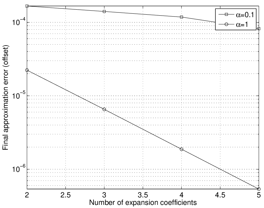
Figure 7 illustrate the error curves for two different choices of the smoothness parameter: panel (a) shows α=0.1\alpha=0.1, whereas panel (b) shows α=1\alpha=1. For the larger value of α\alpha shown in panel (b), the messages in the BP algorithm are smoother, so that the SOSMP estimates are more accurate with the same number of expansion coefficients. Moreover, similar to what we have observed previously, the error decays with the rate of 1/t1/t till it hits the error floor. Note that this error floor is lower for the smoother kernel (α=1\alpha=1) compared to the rougher case (α=0.1\alpha=0.1); note the difference in axis scaling between panels (a) and (b). Moreover, as predicted by our theory, the approximation error decays faster for the smoother kernel, as shown by the plots in Figure 8, in which we plot the final error, due purely to approximation effects, versus the number of expansion coefficients rr. The semilog plot of Figure 8 shows that the resulting lines have different slopes, as would be expected.

Refer to caption Refer to caption
(a) (b)
Figure 7: Plot of the estimation error et/e0e^{t}/e^{0} verses the number of iterations tt for the cases of (a) α=0.1\alpha=0.1 and (b) α=1\alpha=1. The BP messages are smoother when α=1\alpha=1, and accordingly the SOSMP estimates are more accurate with the same number of expansion coefficients. Moreover, the error decays with the rate of 1/t1/t till it hits a floor corresponding to the approximation error incurred by truncating the message expansion coefficients.
Refer to caption
Figure 8: Final approximation error vs. the number of expansion coefficients for the cases of α=0.1\alpha=0.1 and α=1\alpha=1. As predicted by the theory, the error floor decays with a faster pace for the smoother edge potential.

5.2 Computer Vision Application

Refer to caption Refer to caption
(a) (b)
Figure 9: Two frames, each of dimension 250×250250\times 250 pixels, taken from a video sequence of moving cars.

Moving beyond simulated problems, we conclude by showing the SOSMP algorithm in application to a larger scale problem that arises in computer vision—namely, that of optical flow estimation [4]. In this problem, the input data are two successive frames of a video sequence. We model each frame as a collection of pixels arrayed over a n×n\sqrt{n}\times\sqrt{n} grid, and measured intensity values at each pixel location of the form {I⁡(i,j),I′​(i,j)}i,j=1n\{I(i,j),I^{\prime}(i,j)\}_{i,j=1}^{\sqrt{n}}. Our goal is to estimate a 2-dimensional motion vector xu=(xu;1,xu;2)x_{u}=(x_{u;1},x_{u;2}) that captures the local motion at each pixel u=(i,j)u=(i,j), i,j=1,2,…,ni,j=1,2,\ldots,\sqrt{n} of the image sequence.

In order to cast this optical flow problem in terms of message-passing on a graph, we adopt the model used by Boccignone et al. [5]. We model the local motion XuX_{u} as a 22-dimensional random vector taking values in the space 𝒳=[−d,d]×[−d,d]\mathcal{X}=[-d,d]\times[-d,d], and associate the random vector XuX_{u} with vertex uu, in a 2-dimensional grid (see Figure 1(a)). At node u=(i,j)u=(i,j), we use the change between the two image frames to specify the node potential

ψu​(xu;1,xu;2)∝exp⁡(−(I⁡(i,j)−I′​(i+xu;1,j+xu;2))22​σu2).\displaystyle\psi_{u}(x_{u;1},x_{u;2})\;\propto\;\exp\bigg(-\frac{(I(i,j)-I^{\prime}(i+x_{u;1},\;j+x_{u;2}))^{2}}{2\sigma_{u}^{2}}\bigg).

On each edge (u,v)(u,v), we introduce the potential function

ψu​v​(xu,xv)∝exp⁡(−‖xu−xv‖22​σu​v2),\displaystyle\psi_{uv}(x_{u},x_{v})\;\propto\;\exp\bigg(-\frac{\|x_{u}-x_{v}\|^{2}}{2\sigma_{uv}^{2}}\bigg),

which enforces a type of smoothness prior over the image.

To estimate the motion of a truck, we applied the SOSMP algorithm using the 22-dimensional Fourier expansion as our orthonormal basis to two 250×250250\times 250 frames from a truck video sequence (see Figure 9). We apply the SOSMP algorithm using the first r=9r=9 coefficients and k=3k=3 samples. Figure 10 shows the HSV (hue, saturation, value) codings of the estimated motions after t=1,10,40t=1,10,40 iterations, in panels (a), (b) and (c) respectively. (Panel (d) provides an illustration of the HSV encoding: hue is used to represent in the angular direction of the motion whereas the speed (magnitude of the motion) is encoded by the saturation (darker colors meaning higher speeds). The initial estimates of the motion vectors are noisy, but it fairly rapidly converges to a reasonable optical flow field. (To be clear, the purpose of this experiment is not to show the effectiveness of SOSMP or BP as a particular method for optical flow, but rather to demonstrate its correctness and feasibility of the SOSMP in an applied setting.)

Refer to caption Refer to caption
(a) (b)
Refer to caption Refer to caption
(c) (d)
Figure 10: Color coded images of the estimated motion vectors after (a) t=1t=1, (b) t=10t=10, (c) t=40t=40 iterations. Panel (d) illustrates the hsv color coding of the flow. The color hue is used to encode the angular dimension of the motion, whereas the saturation level corresponds to the speed (length of motion vector). We implemented the SOSMP algorithm by expanding in the two-dimensional Fourier basis, using r=9r=9 coefficients and k=3k=3 samples. Although the initial estimates are noisy, it converges to a reasonable optical flow estimate after around 4040 iterations.

6 Proofs

We now turn to the proofs of our main results. They involve a collection of techniques from concentration of measure, stochastic approximation, and functional analysis.

6.1 Proof of Theorem 1

Our goal is to bound the error

‖Δv→ut+1‖L22\displaystyle\|\Delta^{t+1}_{{v}\rightarrow{u}}\|_{L^{2}}^{2}\; =‖mv→ut+1−Πr​(mv→u∗)‖L22=∑j=1r(av→u;jt+1−av→u;j∗)2,\displaystyle=\;\|m^{t+1}_{{v}\rightarrow{u}}-\Pi^{r}(m^{*}_{{v}\rightarrow{u}})\|_{L^{2}}^{2}\;=\;\sum_{j=1}^{r}\big(a^{t+1}_{{v}\rightarrow{u};j}-a^{*}_{{v}\rightarrow{u};j}\big)^{2}, (40)

where the final equality follows by Parseval’s theorem. Here {av→u;j∗}j=1r\{a^{*}_{{v}\rightarrow{u};j}\}_{j=1}^{r} are the basis expansion coefficients that define the best rr approximation to the BP fixed point m∗m^{*}. The following lemma provides an upper bound on this error in terms of two related quantities. First, we let {bv→u;jt}j=1∞\{b_{v\rightarrow u;j}^{t}\}_{j=1}^{\infty} denote the basis function expansion coefficients of the ℱv→u​(m^v→ut)\mathcal{F}_{{{v}\rightarrow{u}}}(\widehat{m}^{t}_{{v}\rightarrow{u}})—that is, [ℱv→u​(m^v→ut)]​(⋅)=∑j=1∞bv→u;jt​ϕj​(⋅)[\mathcal{F}_{{{v}\rightarrow{u}}}(\widehat{m}^{t}_{{v}\rightarrow{u}})](\cdot)=\sum_{j=1}^{\infty}b_{v\rightarrow u;j}^{t}\phi_{j}(\cdot). Second, for each j=1,2,…,rj=1,2,\ldots,r, define the deviation ζv→u;jt+1:=b~v→u;jt+1−bv→u;jt\zeta^{t+1}_{{v}\rightarrow{u};j}:\!\,=\widetilde{b}^{t+1}_{{v}\rightarrow{u};j}-b_{v\rightarrow u;j}^{t}, where the coefficients b~v→u;jt+1\widetilde{b}^{t+1}_{{v}\rightarrow{u};j} are updated in Step 2(c) Figure 3.

Lemma 2.

For each iteration t=0,1,2,…t=0,1,2,\ldots, we have

‖Δv→ut+1‖L22\displaystyle\|\Delta^{t+1}_{{v}\rightarrow{u}}\|_{L^{2}}^{2}\; ≤2t+1​∑j=1r∑τ=0t[bv→u;jτ−av→u;j∗]2⏟Deterministic term Dv→ut+1+2(t+1)2​∑j=1r{∑τ=0tζv→u;jτ+1}2⏟Stochastic term Sv→ut+1\displaystyle\leq\;\underbrace{\frac{2}{t+1}\>\sum_{j=1}^{r}\sum_{\tau=0}^{t}\>\big[b_{v\rightarrow u;j}^{\tau}-a^{*}_{{v}\rightarrow{u};j}\big]^{2}}_{\mbox{Deterministic term $D_{{v}\rightarrow{u}}^{t+1}$}}\,+\,\underbrace{\frac{2}{(t+1)^{2}}\>\sum_{j=1}^{r}\Big\{\sum_{\tau=0}^{t}\zeta^{\tau+1}_{{v}\rightarrow{u};j}\Big\}^{2}}_{\mbox{Stochastic term $S_{{v}\rightarrow{u}}^{t+1}$}} (41)

The proof of this lemma is relatively straightforward; see Appendix A for the details. Note that inequality (41) provides an upper bound on the error that involves two terms: the first term Dv→ut+1D_{{v}\rightarrow{u}}^{t+1} depends only on the expansion coefficients {bv→u;jτ,τ=0,…,t}\{b_{v\rightarrow u;j}^{\tau},\tau=0,\ldots,t\} and the BP fixed point, and therefore is a deterministic quantity when we condition on all randomness in stages up to step tt. The second term Sv→ut+1S_{{v}\rightarrow{u}}^{t+1}, even when conditioned on randomness through step tt, remains stochastic, since the coefficients b~v→ut+1\widetilde{b}^{t+1}_{{v}\rightarrow{u}} (involved in the error term ζv→ut+1\zeta^{t+1}_{{v}\rightarrow{u}}) are updated stochastically in moving from iteration tt to t+1t+1.

We split the remainder of our analysis into three parts: (a) control of the deterministic component; (b) control of the stochastic term; and (c) combining the pieces to provide a convergence bound.

6.1.1 Upper-bounding the deterministic term

By the Pythagorean theorem, we have

∑τ=0t∑j=1r[bv→u;jτ−av→u;j∗]2\displaystyle\sum_{\tau=0}^{t}\sum_{j=1}^{r}\big[b_{v\rightarrow u;j}^{\tau}-a^{*}_{{v}\rightarrow{u};j}\big]^{2}\; ≤∑τ=0t‖ℱv→u​(m^t)−ℱv→u​(m∗)‖L22\displaystyle\leq\;\sum_{\tau=0}^{t}\|\mathcal{F}_{{v}\rightarrow{u}}(\widehat{m}^{t})-\mathcal{F}_{{v}\rightarrow{u}}(m^{*})\|^{2}_{L^{2}} (42)

In order to control this term, we make use of the following lemma, proved in Appendix B:

Lemma 3.

For all directed edges (v→u)∈ℰ→(v\rightarrow u)\in\mathcal{\vec{\mathcal{E}}}, there exist constants {Lv→u;w,w∈𝒩⁡(v)∖{u}}\{L_{{v}\rightarrow{u};w},\mbox{$w\in\mathcal{N}(v)\setminus\{u\}$}\} such that

‖ℱv→u​(m^t)−ℱv→u​(m∗)‖L2\displaystyle\|\mathcal{F}_{{v}\rightarrow{u}}(\widehat{m}^{t})\,-\,\mathcal{F}_{{v}\rightarrow{u}}(m^{*})\|_{L^{2}}\;\; ≤∑w∈𝒩⁡(v)∖{u}Lv→u;w​‖m^w→vt−mw→v∗‖L2\displaystyle\leq\sum_{w\in\mathcal{N}(v)\setminus\{u\}}L_{{v}\rightarrow{u};w}\>\|\widehat{m}^{t}_{{w}\rightarrow{v}}\,-\,m_{{w}\rightarrow{v}}^{\ast}\|_{L^{2}}

for all t=1,2,…t=1,2,\ldots.

Substituting the result of Lemma 3 in equation (42) and performing some algebra, we find that

∑τ=0t∑j=1r[bv→u;jτ−av→u;j∗]2\displaystyle\sum_{\tau=0}^{t}\sum_{j=1}^{r}\big[b_{v\rightarrow u;j}^{\tau}-a^{*}_{{v}\rightarrow{u};j}\big]^{2}\; ≤∑τ=0t(∑w∈𝒩⁡(v)∖{u}Lv→u;w​‖m^w→vτ−mw→v∗‖L2)2\displaystyle\leq\;\sum_{\tau=0}^{t}\Big(\sum_{w\in\mathcal{N}(v)\setminus\{u\}}L_{{v}\rightarrow{u};w}\>\|\widehat{m}^{\tau}_{{w}\rightarrow{v}}\,-\,m_{{w}\rightarrow{v}}^{\ast}\|_{L^{2}}\Big)^{2}
  ≤(dv−1)​∑τ=0t∑w∈𝒩⁡(v)∖{u}Lv→u;w2​‖m^w→vτ−mw→v∗‖L22,\displaystyle\leq\;(d_{v}-1)\;\sum_{\tau=0}^{t}\sum_{w\in\mathcal{N}(v)\setminus\{u\}}L_{{v}\rightarrow{u};w}^{2}\>\|\widehat{m}^{\tau}_{{w}\rightarrow{v}}\,-\,m_{{w}\rightarrow{v}}^{\ast}\|^{2}_{L^{2}}, (43)

where dvd_{v} is the degree of node v∈𝒱v\in\mathcal{V}. By definition, the message m^w→vτ\widehat{m}^{\tau}_{{w}\rightarrow{v}} is the L2L^{2}-projection of mw→vτm^{\tau}_{{w}\rightarrow{v}} onto ℳ\mathcal{M}. Since mw→v∗∈ℳm^{\ast}_{{w}\rightarrow{v}}\in\mathcal{M} and projection is non-expansive, we have

‖m^w→vτ−mw→v∗‖L22\displaystyle\|\widehat{m}^{\tau}_{{w}\rightarrow{v}}\,-\,m_{{w}\rightarrow{v}}^{\ast}\|_{L^{2}}^{2}\; ≤‖mw→vτ−mw→v∗‖L22\displaystyle\leq\;\|m^{\tau}_{{w}\rightarrow{v}}\,-\,m_{{w}\rightarrow{v}}^{\ast}\|_{L^{2}}^{2}
  =‖Δw→vτ‖L22+‖Aw→vr‖L22\displaystyle=\;\|\Delta^{\tau}_{w\rightarrow v}\|_{L^{2}}^{2}\,+\,\|A^{r}_{w\rightarrow v}\|_{L^{2}}^{2} (44)

where in the second step we have used the Pythagorean identity and recalled the definitions of estimation error as well as approximation error from (18) and (19). Substituting the inequality (44) into the bound (43) yields

∑τ=0t∑j=1r[bv→u;jτ−av→u;j∗]2\displaystyle\sum_{\tau=0}^{t}\sum_{j=1}^{r}\big[b_{v\rightarrow u;j}^{\tau}-a^{*}_{{v}\rightarrow{u};j}\big]^{2}\; ≤(dv−1)​∑τ=0t∑w∈𝒩⁡(v)∖{u}Lv→u;w2​(‖Δw→vτ‖L22+‖Aw→vr‖L22).\displaystyle\leq\;(d_{v}-1)\,\sum_{\tau=0}^{t}\sum_{w\in\mathcal{N}(v)\setminus\{u\}}L_{{v}\rightarrow{u};w}^{2}\,\big(\|\Delta^{\tau}_{w\rightarrow v}\|_{L^{2}}^{2}+\|A^{r}_{w\rightarrow v}\|_{L^{2}}^{2}\big).

Therefore, introducing the convenient shorthand L~v→u,w:=2​(dv−1)​Lv→u;w2\widetilde{L}_{{v}\rightarrow{u},w}:\!\,=2\>(d_{v}-1)\>L_{{v}\rightarrow{u};w}^{2}, we have shown that

Dv→ut+1\displaystyle D_{{v}\rightarrow{u}}^{t+1}\; ≤1t+1​∑τ=0t∑w∈𝒩⁡(v)∖{u}L~v→u,w​(‖Δw→vt‖L22+‖Aw→vr‖L22).\displaystyle\leq\;\frac{1}{t+1}\>\sum_{\tau=0}^{t}\;\sum_{w\in\mathcal{N}(v)\setminus\{u\}}\widetilde{L}_{{v}\rightarrow{u},w}\>\big(\|\Delta^{t}_{{w}\rightarrow{v}}\|_{L^{2}}^{2}\,+\,\|A^{r}_{{w}\rightarrow{v}}\|_{L^{2}}^{2}\big). (45)

We make further use of this inequality shortly.

6.1.2 Controlling the stochastic term

We now turn to the stochastic part of the inequality (41). Our analysis is based on the following fact, proved in Appendix C:

Lemma 4.

For each t≥0t\geq 0, let 𝒢t:=σ⁡(m0,…,mt)\mathcal{G}^{t}:\!\,=\sigma(m^{0},\ldots,m^{t}) be the σ\sigma-field generated by all messages through time tt. Then for every fixed j=1,2,…,rj=1,2,\ldots,r, the sequence ζv→u;jt+1=b~v→u;jt+1−bv→u;jt\zeta^{t+1}_{{v}\rightarrow{u};j}=\widetilde{b}^{t+1}_{{v}\rightarrow{u};j}-b_{v\rightarrow u;j}^{t} is a bounded martingale difference with respect to {𝒢t}t=0∞\{\mathcal{G}^{t}\}_{t=0}^{\infty}. In particular, we have |ζv→u;jt+1|≤2​Bj|\zeta^{t+1}_{{v}\rightarrow{u};j}|\leq 2B_{j}, where BjB_{j} was previously defined (24).

Based on Lemma 4, standard martingale convergence results [9] guarantee that for each j=1,2,…,rj=1,2,\ldots,r, we have ∑τ=0tζv→u;jτ+1/(t+1)\sum_{\tau=0}^{t}\zeta^{\tau+1}_{{v}\rightarrow{u};j}/(t+1) converges to 00 almost surely (a.s.) as t→∞t\rightarrow\infty, and hence

Sv→ut+1\displaystyle S_{{v}\rightarrow{u}}^{t+1}\; =2(t+1)2∑j=1r{∑τ=0tζv→u;jτ+1}2= 2∑j=1r{1t+1∑τ=0tζv→u;jτ+1}2⟶a.s.0.\displaystyle=\;\frac{2}{(t+1)^{2}}\>\sum_{j=1}^{r}\>\biggr\{\sum_{\tau=0}^{t}\zeta^{\tau+1}_{{v}\rightarrow{u};j}\;\biggr\}^{2}\;=\;2\>\sum_{j=1}^{r}\>\biggr\{\frac{1}{t+1}\sum_{\tau=0}^{t}\zeta^{\tau+1}_{{v}\rightarrow{u};j}\biggr\}^{2}\;\stackrel{{\scriptstyle\text{a.s.}}}{{\longrightarrow}}0. (46)

Furthermore, we can apply the Azuma-Hoeffding inequality [6] in order to characterize the rate of convergence. For each j=1,2,…,rj=1,2,\ldots,r, define the non-negative random variable Zj:={∑τ=0tζv→u;jτ+1}2/(t+1)2Z_{j}:\!\,=\big\{\sum_{\tau=0}^{t}\zeta^{\tau+1}_{{v}\rightarrow{u};j}\big\}^{2}/(t+1)^{2}. Since |ζv→u;jτ+1|≤2​Bj|\zeta^{\tau+1}_{{v}\rightarrow{u};j}|\leq 2B_{j}, for any δ≥0\delta\geq 0, we have

ℙ[Zj≥δ]\displaystyle\mathbb{P}\big[Z_{j}\geq\delta\big]\; =ℙ[Zj≥δ]≤ 2exp(−(t+1)​δ8​Bj2),\displaystyle=\;\mathbb{P}\big[\sqrt{Z_{j}}\;\geq\;\sqrt{\delta}\big]\;\leq\;2\>\exp\bigg(-\frac{(t+1)\;\delta}{8\>B_{j}^{2}}\bigg),

for all δ>0\delta>0. Moreover, ZjZ_{j} is non-negative; therefore, integrating its tail bound we can compute the expectation

𝔼⁡[Zj]\displaystyle\mathbb{E}[Z_{j}]\; =∫0∞ℙ[Zj≥δ]dδ≤ 2∫0∞exp(−(t+1)​δ8​Bj2)dδ=16​Bj2t+1,\displaystyle=\;\int_{0}^{\infty}\mathbb{P}[Z_{j}\geq\delta]\>d\delta\;\leq\;2\int_{0}^{\infty}\exp\bigg(-\frac{(t+1)\;\delta}{8\>B_{j}^{2}}\bigg)\>d\delta\;=\;\frac{16B_{j}^{2}}{t+1},

and consequently

𝔼⁡[|Sv→ut+1|]≤32​∑j=1rBj2t+1.\displaystyle\mathbb{E}[|S_{{v}\rightarrow{u}}^{t+1}|]\;\leq\;\frac{32\>\sum_{j=1}^{r}B_{j}^{2}}{t+1}. (47)

6.1.3 Establishing convergence

We now make use of the results established so far to prove the claims. Substituting the upper bound (45) on Dv→ut+1D_{{v}\rightarrow{u}}^{t+1} into the decomposition (41) from Lemma 2, we find that

‖Δv→ut+1‖L22\displaystyle\|\Delta^{t+1}_{{v}\rightarrow{u}}\|_{L^{2}}^{2}\; ≤1t+1​∑τ=0t∑w∈𝒩⁡(v)∖{u}L~v→u,w​{‖Δw→vτ‖L22+‖Aw→vr‖L22}+Sv→ut+1.\displaystyle\leq\;\frac{1}{t+1}\>\sum_{\tau=0}^{t}\sum_{w\in\mathcal{N}(v)\setminus\{u\}}\widetilde{L}_{{v}\rightarrow{u},w}\>\big\{\|\Delta^{\tau}_{{w}\rightarrow{v}}\|_{L^{2}}^{2}\,+\,\|A^{r}_{{w}\rightarrow{v}}\|_{L^{2}}^{2}\big\}+S_{{v}\rightarrow{u}}^{t+1}. (48)

For convenience, let us introduce the vector Tt+1={Tv→ut+1,(v→u)∈ℰ→}∈ℝ|ℰ→|T^{t+1}=\{T^{t+1}_{{v}\rightarrow{u}},(v\rightarrow u)\in\mathcal{\vec{\mathcal{E}}}\}\in\mathbb{R}^{|\mathcal{\vec{\mathcal{E}}}|} with entries

Tt+1v→u:=\displaystyle T^{t+1}_{{v}\rightarrow{u}}\;:\!\,= 1t+1​{∑w∈𝒩⁡(v)∖{u}L~v→u,w​‖Δw→v0‖L22}+Sv→ut+1.\displaystyle\;\frac{1}{t+1}\>\Big\{\sum_{w\in\mathcal{N}(v)\setminus\{u\}}\!\!\widetilde{L}_{{v}\rightarrow{u},w}\>\|\Delta^{0}_{{w}\rightarrow{v}}\|_{L^{2}}^{2}\Big\}\,+\,S_{{v}\rightarrow{u}}^{t+1}. (49)

Now define a matix N∈ℝ|ℰ→|×|ℰ→|N\in\mathbb{R}^{|\mathcal{\vec{\mathcal{E}}}|\times|\mathcal{\vec{\mathcal{E}}}|} with entries indexed by the directed edges and set to

Nv→u,w→s\displaystyle N_{{v}\rightarrow{u},\;{w}\rightarrow{s}} :={L~v→u,wif s=v and w∈𝒩⁡(v)∖{u}0otherwise.\displaystyle:\!\,=\;\begin{cases}\widetilde{L}_{{v}\rightarrow{u},w}&\mbox{if $s=v$ and $w\in\mathcal{N}(v)\setminus\{u\}$}\\ 0&\mbox{otherwise.}\end{cases} (50)

In terms of this matrix and the error terms ρ2​(⋅)\rho^{2}\big(\cdot\big) previously defined in equations (21) and (22), the scalar inequalities (48) can be written in the matrix form

ρ2​(Δt+1)\displaystyle\rho^{2}\big(\Delta^{t+1}\big)\; ⪯N⁡[1t+1​∑τ=1tρ2​(Δτ)]+N​ρ2​(Ar)+Tt+1,\displaystyle\preceq\;N\,\Big[\frac{1}{t+1}\>\sum_{\tau=1}^{t}\rho^{2}\big(\Delta^{\tau}\big)\Big]+\,N\,\rho^{2}\big(A^{r}\big)\,+\,T^{t+1}, (51)

where ⪯\preceq denotes the element-wise inequality based on the orthant cone.

From Lemma 1 in the paper [19], the matrix NN is guaranteed to be nilpotent with degree ℓ\ell equal to the graph diameter. Consequently, unwrapping the recursion (51) for a total of ℓ=diam⁡(𝒢)\ell=\operatorname{diam}(\mathcal{G}) times yields

ρ2​(Δt+1)\displaystyle\rho^{2}\big(\Delta^{t+1}\big)\; ⪯T0t+1+N​T1t+1+…+Nℓ−1​Tℓ−1t+1+(N+N2+…+Nℓ)​ρ2​(Ar),\displaystyle\preceq\;T_{0}^{t+1}\,+\,N\>T_{1}^{t+1}\,+\,\ldots\,+\,N^{\ell-1}\>T_{\ell-1}^{t+1}\,+\,(N\,+\,N^{2}\,+\,\ldots\,+\,N^{\ell})\>\rho^{2}\big(A^{r}\big),

where we define T0t+1≡Tt+1T_{0}^{t+1}\equiv T^{t+1}, and then recursively Tst+1:=(∑τ=1tTs−1τ)/(t+1)T_{s}^{t+1}:\!\,=(\sum_{\tau=1}^{t}T_{s-1}^{\tau})/(t+1) for s=1,2,…,ℓ−1s=1,2,\ldots,\ell-1. By the nilpotency of NN, we have the identity I+N+…+Nℓ−1=(I−N)−1I+N+\ldots+N^{\ell-1}=(I-N)^{-1}; so we can further simplify the last inequality

ρ2​(Δt+1)\displaystyle\rho^{2}\big(\Delta^{t+1}\big)\; ⪯∑s=0ℓ−1Ns​Tst+1+N​(I−N)−1​ρ2​(Ar).\displaystyle\preceq\;\sum_{s=0}^{\ell-1}N^{s}\>T_{s}^{t+1}\,+\,N\>(I-N)^{-1}\>\rho^{2}\big(A^{r}\big). (52)

Recalling the definition ℬ:={e∈ℝ|ℰ→|∣|e|⪯N​(I−N)−1​ρ2​(Ar)}\mathcal{B}:\!\,=\big\{e\in\mathbb{R}^{|\mathcal{\vec{\mathcal{E}}}|}\,\mid\,|e|\preceq N(I-N)^{-1}\rho^{2}\big(A^{r}\big)\big\}, inequality (52) implies that

|ρ2​(Δt+1)−Πℬ​(ρ2​(Δt+1))|\displaystyle\big|\rho^{2}\big(\Delta^{t+1}\big)\,-\,\Pi_{\mathcal{B}}\big(\rho^{2}\big(\Delta^{t+1}\big)\big)\big| ⪯∑s=0ℓ−1Ns​Tst+1.\displaystyle\preceq\;\sum_{s=0}^{\ell-1}\>N^{s}\>T_{s}^{t+1}. (53)

We now use the bound (53) to prove both parts of Theorem 1.

Proof of Theorem 1(a):

To prove the almost sure convergence claim in part (a), it suffices to show that for each s=0,1,…,ℓ−1s=0,1,\ldots,\ell-1, we have Tst⟶a.s.0T_{s}^{t}\stackrel{{\scriptstyle\text{a.s.}}}{{\longrightarrow}}0 as t→+∞t\rightarrow+\infty. From equation (46) we know Sv→ut+1→0S_{{v}\rightarrow{u}}^{t+1}\to 0 almost surely as t→∞t\to\infty. In addition, the first term in (49) is at most 𝒪⁡(1/t)\mathcal{O}(1/t), so that also converges to zero as t→∞t\to\infty. Therefore, we conclude that T0t⟶a.s.0T_{0}^{t}\stackrel{{\scriptstyle\text{a.s.}}}{{\longrightarrow}}0 as t→∞t\to\infty.

In order to extend this argument to higher-order terms, let us recall the following elementary fact from real analysis [22]: for any sequence of real numbers {xt}t=0∞\{x^{t}\}_{t=0}^{\infty} such that xt→0x^{t}\to 0, then we also have (∑τ=0txτ)/t→0(\sum_{\tau=0}^{t}x^{\tau})/t\to 0. In order to apply this fact, we observe that T0t⟶a.s.0T_{0}^{t}\stackrel{{\scriptstyle\text{a.s.}}}{{\longrightarrow}}0 means that for almost every sample point ω\omega the deterministic sequence {T0t+1​(ω)}t=0∞\{T_{0}^{t+1}(\omega)\}_{t=0}^{\infty} converges to zero. Consequently, the above fact implies that T1t+1​(ω)=(∑τ=1tT0τ​(ω))/(t+1)→0T_{1}^{t+1}(\omega)=(\sum_{\tau=1}^{t}T_{0}^{\tau}(\omega))/(t+1)\to 0 as t→∞t\to\infty for almost all sample points ω\omega, which is equivalent to asserting that T1t⟶a.s.0→T_{1}^{t}\stackrel{{\scriptstyle\text{a.s.}}}{{\longrightarrow}}\vec{0}. Iterating the same argument, we establish Tst+1⟶a.s.0→T_{s}^{t+1}\stackrel{{\scriptstyle\text{a.s.}}}{{\longrightarrow}}\vec{0} for all s=0,1,…,ℓ−1s=0,1,\ldots,\ell-1, thereby concluding the proof of Theorem 1(a).

Proof of Theorem 1(b):

Taking the expectation on both sides of the inequality (52) yields

𝔼⁡[|ρ2​(Δt+1)−Πℬ​(ρ2​(Δt+1))|]\displaystyle\mathbb{E}\big[|\rho^{2}\big(\Delta^{t+1}\big)-\Pi_{\mathcal{B}}\big(\rho^{2}\big(\Delta^{t+1}\big)\big)|\big]\; ⪯∑s=0ℓ−1Ns​𝔼​[Tst+1].\displaystyle\preceq\;\sum_{s=0}^{\ell-1}N^{s}\>\mathbb{E}[T_{s}^{t+1}]. (54)

so that it suffices to upper bound the expectations 𝔼⁡[Tst+1]\mathbb{E}[T_{s}^{t+1}] for s=0,1,…,ℓ−1s=0,1,\ldots,\ell-1. In Appendix D, we prove the following result:

Lemma 5.

Define the |ℰ→||\mathcal{\vec{\mathcal{E}}}|-vector v→:={∑j=1rBj2}​(2​N​1→+32)\vec{v}:\!\,=\big\{\sum_{j=1}^{r}B_{j}^{2}\big\}(2N\vec{1}+32). Then for all s=0,1,…,ℓ−1s=0,1,\ldots,\ell-1 and t=0,1,2,…t=0,1,2,\ldots,

𝔼⁡[Tst+1]⪯\displaystyle\mathbb{E}[T_{s}^{t+1}]\;\preceq v→t+1​(∑u=0s(log⁡(t+1))uu!),\displaystyle\;\frac{\vec{v}}{t+1}\>\bigg(\sum_{u=0}^{s}\frac{(\log(t+1))^{u}}{u!}\bigg), (55)

Using this lemma, the proof of part (b) follows easily. In particular, substituting the bounds (55) into equation (54) and doing some algebra yields

𝔼⁡[|ρ2​(Δt+1)−Πℬ​(ρ2​(Δt+1))|]⪯\displaystyle\mathbb{E}\big[|\rho^{2}\big(\Delta^{t+1}\big)\,-\,\Pi_{\mathcal{B}}\big(\rho^{2}\big(\Delta^{t+1}\big)\big)|\big]\;\preceq ∑s=0ℓ−1Ns​∑u=0s(log⁡(t+1))uu!​(v→t+1)\displaystyle\;\sum_{s=0}^{\ell-1}N^{s}\sum_{u=0}^{s}\frac{(\log(t+1))^{u}}{u!}\,\Big(\frac{\vec{v}}{t+1}\Big)
⪯\displaystyle\;\preceq  3​∑s=0ℓ−1(log⁡(t+1))s​Ns​(v→t+1)\displaystyle\;3\>\sum_{s=0}^{\ell-1}(\log{(t+1)})^{s}\>N^{s}\,\Big(\frac{\vec{v}}{t+1}\Big)
⪯\displaystyle\;\preceq  3​(I−log⁡(t+1)​N)−1​(v→t+1),\displaystyle\;3\>(I\,-\,\log{(t+1)}\>N)^{-1}\,\Big(\frac{\vec{v}}{t+1}\Big),

where again we used the fact that Nℓ=0N^{\ell}=0.

6.2 Proof of Theorem 2

Recall the definition of the estimation error Δv→ut\Delta^{t}_{{v}\rightarrow{u}} from (18). By Parseval’s identity we know that ‖Δv→ut‖L22=∑j=1r(av→u;jt−av→u;j∗)2\|\Delta^{t}_{{v}\rightarrow{u}}\|_{L^{2}}^{2}=\sum_{j=1}^{r}(a^{t}_{{v}\rightarrow{u};j}-a^{*}_{{v}\rightarrow{u};j})^{2}. For convenience, we introduce the following shorthands for mean squared error on the directed edge (v→u)(v\rightarrow u)

  ​ρ2​(Δv→ut):=𝔼⁡[‖Δv→ut‖L22]=𝔼⁡[∑j=1r(av→u;jt−av→u;j∗)2],\displaystyle\makebox[0.0pt][l]{\hskip 1.29167pt\hskip 0.58333pt\rule[5.59721pt]{3.13037pt}{0.43057pt}}{\rho}^{2}(\Delta^{t}_{{v}\rightarrow{u}})\;:\!\,=\;\mathbb{E}[\|\Delta^{t}_{{v}\rightarrow{u}}\|_{L^{2}}^{2}]\;=\;\mathbb{E}\big[\sum_{j=1}^{r}(a^{t}_{{v}\rightarrow{u};j}-a^{*}_{{v}\rightarrow{u};j})^{2}\big],

as well as the ℓ∞\ell_{\infty} error

  ​ρmax2​(Δt):=max(v→u)∈ℰ→⁡𝔼⁡[‖Δv→ut‖L22],\displaystyle\makebox[0.0pt][l]{\hskip 1.29167pt\hskip 0.58333pt\rule[5.59721pt]{3.13037pt}{0.43057pt}}{\rho}^{2}_{\tiny{\mbox{max}}}(\Delta^{t})\;:\!\,=\;\max_{(v\rightarrow u)\in\mathcal{\vec{\mathcal{E}}}}\mathbb{E}[\|\Delta^{t}_{{v}\rightarrow{u}}\|_{L^{2}}^{2}],

similarly defined for approximation error

ρmax2​(Ar):=max(v→u)∈ℰ→⁡‖Av→ur‖L22.\displaystyle\rho^{2}_{\tiny{\mbox{max}}}(A^{r})\;:\!\,=\;\max_{(v\rightarrow u)\in\mathcal{\vec{\mathcal{E}}}}\|A^{r}_{{{v}\rightarrow{u}}}\|_{L^{2}}^{2}.

Using the definition of   ​ρ2​(Δv→ut)\makebox[0.0pt][l]{\hskip 1.29167pt\hskip 0.58333pt\rule[5.59721pt]{3.13037pt}{0.43057pt}}{\rho}^{2}(\Delta^{t}_{{v}\rightarrow{u}}), some algebra yields

  ​ρ2​(Δv→ut+1)−  ​ρ2​(Δv→ut)\displaystyle\makebox[0.0pt][l]{\hskip 1.29167pt\hskip 0.58333pt\rule[5.59721pt]{3.13037pt}{0.43057pt}}{\rho}^{2}(\Delta^{t+1}_{{v}\rightarrow{u}})-\makebox[0.0pt][l]{\hskip 1.29167pt\hskip 0.58333pt\rule[5.59721pt]{3.13037pt}{0.43057pt}}{\rho}^{2}(\Delta^{t}_{{v}\rightarrow{u}})\; =𝔼⁡[∑j=1r(av→u;jt+1−av→u;j∗)2−∑j=1r(av→u;jt−av→u;j∗)2]\displaystyle=\;\mathbb{E}\Big[\sum_{j=1}^{r}\big(a^{t+1}_{{v}\rightarrow{u};j}-a^{*}_{{v}\rightarrow{u};j}\big)^{2}\,-\,\sum_{j=1}^{r}\big(a^{t}_{{v}\rightarrow{u};j}-a^{*}_{{v}\rightarrow{u};j}\big)^{2}\Big]
=𝔼⁡[∑j=1r{av→u;jt+1−av→u;jt}​{(av→u;jt+1−av→u;jt)+ 2​(av→u;jt−av→u;j∗)}].\displaystyle=\;\mathbb{E}\Big[\sum_{j=1}^{r}\big\{a^{t+1}_{{v}\rightarrow{u};j}-a^{t}_{{v}\rightarrow{u};j}\big\}\;\big\{\big(a^{t+1}_{{v}\rightarrow{u};j}-a^{t}_{{v}\rightarrow{u};j}\big)\,+\,2\big(a^{t}_{{v}\rightarrow{u};j}-a^{*}_{{v}\rightarrow{u};j}\big)\big\}\Big].

From the update equation (16), we have

av→u;jt+1−av→u;jt\displaystyle a^{t+1}_{{v}\rightarrow{u};j}-a^{t}_{{v}\rightarrow{u};j}\; =ηt​(b~v→u;jt+1−av→u;jt),\displaystyle=\;\eta^{t}\>\big(\widetilde{b}^{t+1}_{{v}\rightarrow{u};j}-a^{t}_{{v}\rightarrow{u};j}\big),

and hence

  ​ρ2​(Δv→ut+1)−  ​ρ2​(Δv→ut)=Uv→ut+Vv→ut,\displaystyle\makebox[0.0pt][l]{\hskip 1.29167pt\hskip 0.58333pt\rule[5.59721pt]{3.13037pt}{0.43057pt}}{\rho}^{2}(\Delta^{t+1}_{{v}\rightarrow{u}})-\makebox[0.0pt][l]{\hskip 1.29167pt\hskip 0.58333pt\rule[5.59721pt]{3.13037pt}{0.43057pt}}{\rho}^{2}(\Delta^{t}_{{v}\rightarrow{u}})\;=\;U^{t}_{{v}\rightarrow{u}}+V^{t}_{{v}\rightarrow{u}}, (56)

where

Uv→ut\displaystyle U^{t}_{{v}\rightarrow{u}}\; :=(ηt)2​∑j=1r𝔼⁡[(b~v→u;jt+1−av→u;jt)2],and\displaystyle:\!\,=\;(\eta^{t})^{2}\sum_{j=1}^{r}\>\mathbb{E}\,\big[\big(\widetilde{b}^{t+1}_{{v}\rightarrow{u};j}-a^{t}_{{v}\rightarrow{u};j}\big)^{2}\big],\quad\mbox{and} (57a)
Vv→ut\displaystyle V^{t}_{{v}\rightarrow{u}}\; := 2​ηt​∑j=1r𝔼⁡[(b~v→u;jt+1−av→u;jt)​(av→u;jt−av→u;j∗)].\displaystyle:\!\,=\;2\eta^{t}\,\sum_{j=1}^{r}\>\mathbb{E}\>\Big[\big(\widetilde{b}^{t+1}_{{v}\rightarrow{u};j}-a^{t}_{{v}\rightarrow{u};j}\big)\,\big(a^{t}_{{v}\rightarrow{u};j}-a^{*}_{{v}\rightarrow{u};j}\big)\Big]. (57b)

The following lemma, proved in Appendix E, provides upper bounds on these two terms.

Lemma 6.

For all iterations t=0,1,2,…t=0,1,2,\ldots, we have

Uv→ut\displaystyle U^{t}_{{v}\rightarrow{u}}\; ≤ 4​(ηt)2​∑j=1rBj2,and\displaystyle\leq\;4(\eta^{t})^{2}\>\sum_{j=1}^{r}B_{j}^{2},\quad\mbox{and} (58a)
Vv→ut\displaystyle V^{t}_{{v}\rightarrow{u}}\; ≤ηt​(1−γ2)​ρmax2​(Ar)+ηt​(1−γ2)​  ​ρmax2​(Δt)−ηt​(1+γ2)​  ​ρ2​(Δv→ut).\displaystyle\leq\;\eta^{t}\big(1-\frac{\gamma}{2}\big)\rho^{2}_{\tiny{\mbox{max}}}(A^{r})\,+\,\eta^{t}\big(1-\frac{\gamma}{2}\big)\makebox[0.0pt][l]{\hskip 1.29167pt\hskip 0.58333pt\rule[5.59721pt]{3.13037pt}{0.43057pt}}{\rho}^{2}_{\tiny{\mbox{max}}}(\Delta^{t})\,-\,\eta^{t}(1+\frac{\gamma}{2})\makebox[0.0pt][l]{\hskip 1.29167pt\hskip 0.58333pt\rule[5.59721pt]{3.13037pt}{0.43057pt}}{\rho}^{2}(\Delta^{t}_{{v}\rightarrow{u}}). (58b)

We continue upper-bounding   ​ρ2​(Δv→ut+1)\makebox[0.0pt][l]{\hskip 1.29167pt\hskip 0.58333pt\rule[5.59721pt]{3.13037pt}{0.43057pt}}{\rho}^{2}(\Delta^{t+1}_{{v}\rightarrow{u}}) by substituting the results of Lemma 6 into equation (56), thereby obtaining

  ​ρ2​(Δv→ut+1)\displaystyle\makebox[0.0pt][l]{\hskip 1.29167pt\hskip 0.58333pt\rule[5.59721pt]{3.13037pt}{0.43057pt}}{\rho}^{2}(\Delta^{t+1}_{{v}\rightarrow{u}})\; ≤ 4​(ηt)2​∑j=1rBj2+ηt​(1−γ2)​ρmax2​(Ar)+ηt​(1−γ2)​  ​ρmax2​(Δt)+{1−ηt​(1+γ2)}​  ​ρ2​(Δv→ut)\displaystyle\leq\;4(\eta^{t})^{2}\sum_{j=1}^{r}B_{j}^{2}\,+\,\eta^{t}\big(1-\frac{\gamma}{2}\big)\>\rho^{2}_{\tiny{\mbox{max}}}(A^{r})\,+\,\eta^{t}\big(1-\frac{\gamma}{2}\big)\>\makebox[0.0pt][l]{\hskip 1.29167pt\hskip 0.58333pt\rule[5.59721pt]{3.13037pt}{0.43057pt}}{\rho}^{2}_{\tiny{\mbox{max}}}(\Delta^{t})\,+\,\Big\{1-\eta^{t}(1+\frac{\gamma}{2})\Big\}\makebox[0.0pt][l]{\hskip 1.29167pt\hskip 0.58333pt\rule[5.59721pt]{3.13037pt}{0.43057pt}}{\rho}^{2}(\Delta^{t}_{{v}\rightarrow{u}})
≤ 4​(ηt)2​∑j=1rBj2+ηt​(1−γ2)​ρmax2​(Ar)+(1−ηt​γ)​  ​ρmax2​(Δt).\displaystyle\leq\;4(\eta^{t})^{2}\sum_{j=1}^{r}B_{j}^{2}\,+\,\eta^{t}\big(1-\frac{\gamma}{2}\big)\rho^{2}_{\tiny{\mbox{max}}}(A^{r})\,+\,\big(1-\eta^{t}\gamma\big)\makebox[0.0pt][l]{\hskip 1.29167pt\hskip 0.58333pt\rule[5.59721pt]{3.13037pt}{0.43057pt}}{\rho}^{2}_{\tiny{\mbox{max}}}(\Delta^{t}).

Since this equation holds for all directed edges (v→u)(v\rightarrow u), taking the maximum over the left-hand side yields the recursion

  ​ρmax2​(Δt+1)\displaystyle\makebox[0.0pt][l]{\hskip 1.29167pt\hskip 0.58333pt\rule[5.59721pt]{3.13037pt}{0.43057pt}}{\rho}^{2}_{\tiny{\mbox{max}}}(\Delta^{t+1})\; ≤(ηt)2​  ​B2+ηt​(1−γ2)​ρmax2​(Ar)+(1−ηt​γ)​  ​ρmax2​(Δt),\displaystyle\leq\;(\eta^{t})^{2}\,\makebox[0.0pt][l]{\hskip 2.05pt\hskip 0.0pt\rule[8.12498pt]{5.73494pt}{0.43057pt}}{B}^{2}\,+\,\eta^{t}\big(1-\frac{\gamma}{2}\big)\>\rho^{2}_{\tiny{\mbox{max}}}(A^{r})\,+\,\big(1-\eta^{t}\gamma\big)\>\makebox[0.0pt][l]{\hskip 1.29167pt\hskip 0.58333pt\rule[5.59721pt]{3.13037pt}{0.43057pt}}{\rho}^{2}_{\tiny{\mbox{max}}}(\Delta^{t}), (59)

where we have introduced the shorthand   ​B2=4​∑j=1rBj2\makebox[0.0pt][l]{\hskip 2.05pt\hskip 0.0pt\rule[8.12498pt]{5.73494pt}{0.43057pt}}{B}^{2}=4\sum_{j=1}^{r}B_{j}^{2}. Setting ηt=1/(γ⁡(t+1))\eta^{t}=1/(\gamma\,(t+1)) and unwrapping this recursion, we find that

  ​ρmax2​(Δt+1)\displaystyle\makebox[0.0pt][l]{\hskip 1.29167pt\hskip 0.58333pt\rule[5.59721pt]{3.13037pt}{0.43057pt}}{\rho}^{2}_{\tiny{\mbox{max}}}(\Delta^{t+1})\; ≤  ​B2γ2​∑τ=1t+11τ⁡(t+1)+2−γ2​γ​ρmax2​(Ar)\displaystyle\leq\;\frac{\makebox[0.0pt][l]{\hskip 2.05pt\hskip 0.0pt\rule[8.12498pt]{5.73494pt}{0.43057pt}}{B}^{2}}{\gamma^{2}}\sum_{\tau=1}^{t+1}\frac{1}{\tau\,(t+1)}\,+\,\frac{2-\gamma}{2\gamma}\,\rho^{2}_{\tiny{\mbox{max}}}(A^{r})
≤2​  ​B2γ2​log⁡(t+1)t+1+1γ​ρmax2​(Ar),\displaystyle\leq\;\frac{2\,\makebox[0.0pt][l]{\hskip 2.05pt\hskip 0.0pt\rule[8.12498pt]{5.73494pt}{0.43057pt}}{B}^{2}}{\gamma^{2}}\;\frac{\log(t+1)}{t+1}\,+\,\frac{1}{\gamma}\,\rho^{2}_{\tiny{\mbox{max}}}(A^{r}),

which establishes the claim.

6.3 Proof of Theorem 3

As discussed earlier, each iteration of the SOSMP algorithm requires 𝒪⁡(r)\mathcal{O}(r) operations per edge. Consequently, it suffices to show that running the algorithm with r=r∗r=r^{*} coefficients for (∑j=1rλj2)​(1/δ)​log⁡(1/δ)(\sum_{j=1}^{r}\lambda_{j}^{2})(1/\delta)\log(1/\delta) iterations suffices to achieve mean-squared error less than δ\delta.

The bound (28) consists of two terms. In order to characterize the first term (estimation error), we need to bound BjB_{j} defined in (24). Using the orthonormality of the basis functions and the fact that the supremum is attainable over the compact space 𝒳\mathcal{X}, we obtain

Bj=max⁡supy∈𝒳(v→u)∈ℰ→⁡λj​ϕj​(y)∫𝒳ψu​v​(x,y)​μ​(𝑑x)=𝒪⁡(λj).\displaystyle B_{j}\;=\;\max_{(v\rightarrow u)\in\mathcal{\vec{\mathcal{E}}}}\sup_{y\in\mathcal{X}}\;\frac{\lambda_{j}\>\phi_{j}(y)}{\int_{\mathcal{X}}\psi_{uv}(x,y)\mu(dx)}\;=\;\mathcal{O}(\lambda_{j}).

Therefore, the estimation error decays at the rate 𝒪⁡((∑j=1rλj2)​(log⁡t/t))\mathcal{O}\big((\sum_{j=1}^{r}\lambda_{j}^{2})\>(\log{t}/t)\big), so that t=𝒪⁡((∑j=1rλj2)​(1/δ)​log⁡(1/δ))t=\mathcal{O}\big((\sum_{j=1}^{r}\lambda_{j}^{2})(1/\delta)\log(1/\delta)\big) iterations are sufficient to reduce it to 𝒪⁡(δ)\mathcal{O}(\delta).

The second term (approximation error) in the bound (28) depends only on the choice of rr, and in particular on the rr-term approximation error ‖Av→ur‖L22=‖mv→u∗−Πr​(mv→u∗)‖L22\|A^{r}_{{v}\rightarrow{u}}\|_{L^{2}}^{2}=\|m^{*}_{{v}\rightarrow{u}}-\Pi^{r}(m^{*}_{{v}\rightarrow{u}})\|_{L^{2}}^{2}. To bound this term, we begin by representing mv→u∗m^{*}_{{v}\rightarrow{u}} in terms of the basis expansion ∑j=1∞aj∗​ϕj\sum_{j=1}^{\infty}a^{*}_{j}\phi_{j}. By the Pythagorean theorem, we have

‖mv→u∗−Πr​(mv→u∗)‖L22\displaystyle\|m^{*}_{{v}\rightarrow{u}}-\Pi^{r}(m^{*}_{{v}\rightarrow{u}})\|_{L^{2}}^{2} =∑j=r+1∞(aj∗)2.\displaystyle=\sum_{j=r+1}^{\infty}(a^{*}_{j})^{2}. (60)

Our first claim is that ∑j=1∞(aj∗)2/λj<∞\sum_{j=1}^{\infty}(a^{*}_{j})^{2}/\lambda_{j}<\infty. Indeed, since m∗m^{*} is a fixed point of the message update equation, we have

mv→u∗​(⋅)∝∫𝒳ψu​v​(⋅,xv)​M​(xv)​μ​(d​xv),\displaystyle m^{*}_{{{v}\rightarrow{u}}}(\cdot)\;\propto\;\int_{\mathcal{X}}\psi_{uv}(\cdot,x_{v})\,M(x_{v})\,\mu(dx_{v}),

where M⁡(⋅):=ψv​(⋅)​∏w∈𝒩⁡(v)∖{u}mw→v∗​(⋅)M(\cdot):\!\,=\psi_{v}(\cdot)\prod_{w\in\mathcal{N}(v)\setminus\{u\}}m^{*}_{{w}\rightarrow{v}}(\cdot). Exchanging the order of integrations using Fubini’s theorem, we obtain

aj∗=⟨mv→u∗,ϕj⟩L2\displaystyle a^{*}_{j}\;=\;\langle m^{*}_{{{v}\rightarrow{u}}},\,\phi_{j}\rangle_{L^{2}}\; ∝∫𝒳⟨ϕj​(⋅),ψu​v​(⋅,xv)⟩L2​M​(xv)​μ​(d​xv).\displaystyle\propto\;\int_{\mathcal{X}}\langle\phi_{j}(\cdot),\,\psi_{uv}(\cdot,x_{v})\rangle_{L^{2}}\;M(x_{v})\>\mu(dx_{v}). (61)

By the eigenexpansion of ψu​v\psi_{uv}, we have

⟨ϕj​(⋅),ψu​v​(⋅,xv)⟩L2\displaystyle\langle\phi_{j}(\cdot),\,\psi_{uv}(\cdot,x_{v})\rangle_{L^{2}}\; =∑k=1∞λk​⟨ϕj,ϕk⟩L2​ϕk​(xv)=λj​ϕj​(xv).\displaystyle=\;\sum_{k=1}^{\infty}\lambda_{k}\langle\phi_{j},\,\phi_{k}\rangle_{L^{2}}\;\phi_{k}(x_{v})\;=\;\lambda_{j}\>\phi_{j}(x_{v}).

Substituting back into our initial equation (61), we find that

aj∗\displaystyle a^{*}_{j}\; ∝λj​∫𝒳ϕj​(xv)​M​(xv)​μ​(d​xv)=λj​a~j,\displaystyle\propto\;\lambda_{j}\int_{\mathcal{X}}\phi_{j}(x_{v})\;M(x_{v})\>\mu(dx_{v})\;=\;\lambda_{j}\>\widetilde{a}_{j},

where a~j\widetilde{a}_{j} are the basis expansion coefficients of MM. Since the space 𝒳\mathcal{X} is compact, one can see that M∈L2​(𝒳)M\in L^{2}(\mathcal{X}), and hence ∑j=1∞a~j2<∞\sum_{j=1}^{\infty}\widetilde{a}_{j}^{2}<\infty. Therefore, we have

∑j=1∞(aj∗)2λj\displaystyle\sum_{j=1}^{\infty}\frac{(a^{*}_{j})^{2}}{\lambda_{j}}\; ∝∑j=1∞λj​a~j2<+∞,\displaystyle\propto\;\sum_{j=1}^{\infty}\lambda_{j}\>\widetilde{a}_{j}^{2}\;<\;+\infty,

where we used the fact that ∑j=1∞λj<∞\sum_{j=1}^{\infty}\lambda_{j}<\infty.

We now use this bound to control the approximation error (60). For any r=1,2,…r=1,2,\ldots, we have

∑j=r+1∞(aj∗)2\displaystyle\sum_{j=r+1}^{\infty}(a^{*}_{j})^{2}\; =∑j=r+1∞λj​(aj∗)2λj≤λr​∑j=r+1∞(aj∗)2λj=𝒪⁡(λr),\displaystyle=\;\sum_{j=r+1}^{\infty}\lambda_{j}\;\frac{(a^{*}_{j})^{2}}{\lambda_{j}}\;\leq\;\lambda_{r}\sum_{j=r+1}^{\infty}\frac{(a^{*}_{j})^{2}}{\lambda_{j}}\;=\;\mathcal{O}(\lambda_{r}),

using the non-increasing nature of the sequence {λj}j=1∞\{\lambda_{j}\}_{j=1}^{\infty}. Consequently, by definition of r∗r^{*} (31), we have

‖mv→u∗−Πr∗​(mv→u∗)‖L22\displaystyle\|m^{*}_{{v}\rightarrow{u}}-\Pi^{r^{*}}(m^{*}_{{v}\rightarrow{u}})\|_{L^{2}}^{2} =𝒪⁡(δ),\displaystyle=\mathcal{O}(\delta),

as claimed.

7 Conclusion

Belief propagation is a widely used message-passing algorithm for computing (approximate) marginals in graphical models. In this paper, we have presented and analyzed the SOSMP algorithm for running BP in models with continuous variables. It is based on two forms of approximation: a deterministic approximation that involves projecting messages onto the span of rr basis functions, and a stochastic approximation that involves approximating integrals by Monte Carlo estimates. These approximations, while leading to an algorithm with substantially reduced complexity, are also controlled: we provide upper bounds on the convergence of the stochastic error, showing that it goes to zero as 𝒪⁡(log⁡t/t)\mathcal{O}(\log t/t) with the number of iterations, and also control on the deterministic error. For graphs with relatively smooth potential functions, as reflected in the decay rate of their basis coefficients, we provided a quantitative bound on the total number of basic arithmetic operations required to compute the BP fixed point to within δ\delta-accuracy. We illustrated our theoretical predictions using experiments on simulated graphical models, as well as in a real-world instance of optical flow estimation.

Our work leaves open a number of interesting questions. First, although we have focused exclusively on models with pairwise interactions, it should be possible to develop forms of SOSMP for higher-order factor graphs. Second, the bulk of our analysis was performed under a type of contractivity condition, as has been used in past work [26, 11, 17, 21] on convergence of the standard BP updates. However, we suspect that this condition might be somewhat relaxed, and doing so would demonstrate applicability of the SOSMP algorithm to a larger class of graphical models.

Acknowledgements

This work was partially supported by Office of Naval Research MURI grant N00014-11-1-0688 to MJW. The authors thank Erik Sudderth for helpful discussions and pointers to the literature.

Appendix A Proof of Lemma 2

Subtracting av→u;j∗a^{*}_{{v}\rightarrow{u};j} from both sides of the update (16) in Step 2(c), we obtain

av→u;jt+1−av→u;j∗\displaystyle a^{t+1}_{{v}\rightarrow{u};j}-a^{*}_{{v}\rightarrow{u};j}\; =(1−ηt)​[av→u;jt−av→u;j∗]+ηt​[bv→u;jt−av→u;j∗]+ηt​ζv→u;jt+1.\displaystyle=\;(1-\eta^{t})\,\big[a^{t}_{{v}\rightarrow{u};j}-a^{*}_{{v}\rightarrow{u};j}\big]\,+\,\eta^{t}\>\big[b_{v\rightarrow u;j}^{t}-a^{*}_{{v}\rightarrow{u};j}\big]\,+\,\eta^{t}\>\zeta^{t+1}_{{v}\rightarrow{u};j}. (62)

Setting ηt=1/(t+1)\eta^{t}=1/(t+1) and unwrapping the recursion (62) then yields

av→u;jt+1−av→u;j∗\displaystyle a^{t+1}_{{v}\rightarrow{u};j}-a^{*}_{{v}\rightarrow{u};j}\; =1t+1​∑τ=0t[bv→u;jτ−av→u;j∗]+1t+1​∑τ=0tζv→u;jτ+1.\displaystyle=\;\frac{1}{t+1}\sum_{\tau=0}^{t}\big[b_{v\rightarrow u;j}^{\tau}-a^{*}_{{v}\rightarrow{u};j}\big]\,+\,\frac{1}{t+1}\sum_{\tau=0}^{t}\zeta^{\tau+1}_{{v}\rightarrow{u};j}.

Squaring both sides of this equality and using the upper bound (a+b)2≤2​a2+2​b2(a+b)^{2}\leq 2a^{2}+2b^{2}, we obtain

(av→u;jt+1−av→u;j∗)2\displaystyle\big(a^{t+1}_{{v}\rightarrow{u};j}-a^{*}_{{v}\rightarrow{u};j}\big)^{2}\; ≤2(t+1)2​{∑τ=0t[bv→u;jτ−av→u;j∗]}2+2(t+1)2​{∑τ=0tζv→u;jτ+1}2.\displaystyle\leq\;\frac{2}{(t+1)^{2}}\>\Big\{\sum_{\tau=0}^{t}\>\big[b_{v\rightarrow u;j}^{\tau}-a^{*}_{{v}\rightarrow{u};j}\big]\Big\}^{2}\,+\,\frac{2}{(t+1)^{2}}\>\Big\{\sum_{\tau=0}^{t}\zeta^{\tau+1}_{{v}\rightarrow{u};j}\Big\}^{2}.

Summing over indices j=1,2,…,rj=1,2,\ldots,r and recalling the expansion (40), we find that

‖Δv→ut‖L22\displaystyle\|\Delta^{t}_{{v}\rightarrow{u}}\|_{L^{2}}^{2}\; ≤∑j=1r{2(t+1)2{∑τ=0t[bv→u;jτ−av→u;j∗]}2+2(t+1)2{∑τ=0tζv→u;jτ+1}2}\displaystyle\leq\;\sum_{j=1}^{r}\Biggr\{\frac{2}{(t+1)^{2}}\>\Big\{\sum_{\tau=0}^{t}\>\big[b_{v\rightarrow u;j}^{\tau}-a^{*}_{{v}\rightarrow{u};j}\big]\Big\}^{2}\,+\,\frac{2}{(t+1)^{2}}\>\Big\{\sum_{\tau=0}^{t}\zeta^{\tau+1}_{{v}\rightarrow{u};j}\Big\}^{2}\Biggr\}
≤(i)2(t+1)​∑j=1r∑τ=0t[bv→u;jτ−av→u;j∗]2⏟Deterministic term Dv→ut+1+2(t+1)2​∑j=1r{∑τ=0tζv→u;jτ+1}2.⏟Stochastic term Sv→ut+1\displaystyle\stackrel{{\scriptstyle\mathrm{(i)}}}{{\leq}}\;\underbrace{\frac{2}{(t+1)}\>\sum_{j=1}^{r}\sum_{\tau=0}^{t}\>\big[b_{v\rightarrow u;j}^{\tau}-a^{*}_{{v}\rightarrow{u};j}\big]^{2}}_{\mbox{Deterministic term $D_{{v}\rightarrow{u}}^{t+1}$}}\,+\,\underbrace{\frac{2}{(t+1)^{2}}\>\sum_{j=1}^{r}\Big\{\sum_{\tau=0}^{t}\zeta^{\tau+1}_{{v}\rightarrow{u};j}\Big\}^{2}.}_{\mbox{Stochastic term $S_{{v}\rightarrow{u}}^{t+1}$}}

Here step (i) follows from the elementary inequality

{∑τ=0t[bv→u;jτ−av→u;j∗]}2\displaystyle\Big\{\sum_{\tau=0}^{t}\big[b_{v\rightarrow u;j}^{\tau}-a^{*}_{{v}\rightarrow{u};j}\big]\Big\}^{2}\; ≤(t+1)​∑τ=0t[bv→u;jτ−av→u;j∗]2.\displaystyle\leq\;(t+1)\>\sum_{\tau=0}^{t}\big[b_{v\rightarrow u;j}^{\tau}-a^{*}_{{v}\rightarrow{u};j}\big]^{2}.

Appendix B Proof of Lemma 3

Recall the probability density

[pv→u​(m)]​(⋅)\displaystyle[p_{{v}\rightarrow{u}}(m)](\cdot)\; ∝βu​v​(⋅)​∏w∈𝒩⁡(v)∖{u}mw→v​(⋅)\displaystyle\propto\;\beta_{uv}(\cdot)\;\prod_{w\in\mathcal{N}(v)\setminus\{u\}}\!\!m_{{w}\rightarrow{v}}(\cdot)

defined in Step 2 of the SOSMP algorithm. Using this shorthand notation, the claim of Lemma 1 can be re-written as [ℱv→u​(m)]​(x)=⟨Γu​v​(x,⋅),[pv→u​(m)]​(⋅)⟩L2[\mathcal{F}_{{v}\rightarrow{u}}(m)](x)=\langle\Gamma_{uv}(x,\cdot),\,[p_{{v}\rightarrow{u}}(m)](\cdot)\rangle_{L^{2}}. Therefore, applying the Cauchy-Schwartz inequality yields

|[ℱv→u​(m)]​(x)−[ℱv→u​(m′)]​(x)|2≤‖Γu​v​(x,⋅)‖L22​‖pv→u​(m)−pv→u​(m′)‖L22.\displaystyle|[\mathcal{F}_{{v}\rightarrow{u}}(m)](x)-[\mathcal{F}_{{v}\rightarrow{u}}(m^{\prime})](x)|^{2}\;\leq\;\|\Gamma_{uv}(x,\cdot)\|_{L^{2}}^{2}\;\,\|p_{{v}\rightarrow{u}}(m)\,-\,p_{{v}\rightarrow{u}}(m^{\prime})\|_{L^{2}}^{2}.

Integrating both sides of the previous inequality over 𝒳\mathcal{X} and taking square roots yields

‖ℱv→u​(m)−ℱv→u​(m′)‖L2≤Cu​v​‖pv→u​(m)−pv→u​(m′)‖L2,\displaystyle\|\mathcal{F}_{{v}\rightarrow{u}}(m)\,-\,\mathcal{F}_{{v}\rightarrow{u}}(m^{\prime})\|_{L^{2}}\;\leq\;C_{uv}\>\|p_{{v}\rightarrow{u}}(m)\,-\,p_{{v}\rightarrow{u}}(m^{\prime})\|_{L^{2}},

where we have denoted the constant Cu​v:=(∫𝒳|Γu​v​(x,y)|2​μ​(𝑑y)​μ​(𝑑x))1/2C_{uv}:\!\,=\big(\int_{\mathcal{X}}|\Gamma_{uv}(x,y)|^{2}\mu(dy)\mu(dx)\big)^{1/2}.

Next step would be to upper bound the term ‖pv→u​(m)−pv→u​(m′)‖L2\|p_{{v}\rightarrow{u}}(m)-p_{{v}\rightarrow{u}}(m^{\prime})\|_{L^{2}}. In order to do so, we first show that pv→u​(m)p_{{v}\rightarrow{u}}(m) is a Frechet differentiable operator on the space ℳ′:=convhull{m∗,⊕(v→u)∈ℰ→ℳv→u′}\mathcal{M}^{\prime}:\!\,=\operatorname{convhull}\{m^{\ast},\oplus_{(v\to u)\in\mathcal{\vec{\mathcal{E}}}}\>\mathcal{M}^{\prime}_{{{v}\rightarrow{u}}}\}, where

ℳv→u′:={m^v→u|m^v→u=[𝔼Y∼f[Πr(Γu​v(⋅,Y))]]+,for some probability density f},\displaystyle\mathcal{M}^{\prime}_{{{v}\rightarrow{u}}}\;:\!\,=\;\Big\{\widehat{m}_{{{v}\rightarrow{u}}}\>\Big|\>\widehat{m}_{{{v}\rightarrow{u}}}=\Big[\mathbb{E}_{Y\sim f}\big[\Pi^{r}\big(\Gamma_{uv}(\cdot,Y)\big)\big]\Big]_{+},\;\text{for some probability density $f$}\Big\},

denotes the space of all feasible SOSMP messages on the directed edge (v→u)(v\rightarrow u). Doing some calculus using the chain rule, we calculate the partial directional (Gateaux) derivative of the operator pv→u​(m)p_{{v}\rightarrow{u}}(m) with respect to the function mw→vm_{{w}\rightarrow{v}}. More specifically, for an arbitrary function hw→vh_{w\rightarrow v}, we have

[𝒟w​pv→u​(m)]​(hw→v)=\displaystyle[\mathcal{D}_{w}\>p_{{{v}\rightarrow{u}}}(m)](h_{w\rightarrow v})\;= βu​v​∏s∈𝒩⁡(v)∖{u,w}ms→v⟨Mu​v,βu​v⟩L2​hw→v\displaystyle\;\frac{\beta_{uv}\prod_{s\in\mathcal{N}(v)\setminus\{u,w\}}m_{{s}\rightarrow{v}}}{\langle M_{uv},\,\beta_{uv}\rangle_{L^{2}}}\;h_{w\rightarrow v}
−βu​v​Mu​v⟨Mu​v,βu​v⟩L22​⟨hw→v,βu​v​∏s∈𝒩⁡(v)∖{u,w}ms→v⟩L2,\displaystyle-\,\frac{\beta_{uv}M_{uv}}{\langle M_{uv},\,\beta_{uv}\rangle_{L^{2}}^{2}}\;\langle h_{w\rightarrow v},\,\beta_{uv}\!\!\!\!\prod_{s\in\mathcal{N}(v)\setminus\{u,w\}}\!\!\!\!m_{{s}\rightarrow{v}}\rangle_{L^{2}},

where Mu​v=∏w∈𝒩⁡(v)∖{u}mw→vM_{uv}=\prod_{w\in\mathcal{N}(v)\setminus\{u\}}m_{{w}\rightarrow{v}}. Clearly the Gateaux derivative is linear and continuous. It is also bounded as will be shown now. Massaging the operator norm’s definition, we obtain

supm∈ℳ′‖|𝒟w​pv→u​(m)|‖2=\displaystyle\sup_{m\in\mathcal{M}^{\prime}}|\!|\!|\mathcal{D}_{w}\>p_{{{v}\rightarrow{u}}}(m)|\!|\!|_{2}\;= supm∈ℳ′suphw→v∈ℳw→v′‖[𝒟w​pv→u​(m)]​(hw→v)‖L2‖hw→v‖L2\displaystyle\;\sup_{m\in\mathcal{M}^{\prime}}\sup_{h_{w\rightarrow v}\in\mathcal{M}^{\prime}_{{w}\rightarrow{v}}}\frac{\|[\mathcal{D}_{w}\>p_{{{v}\rightarrow{u}}}(m)](h_{w\rightarrow v})\|_{L^{2}}}{\|h_{w\rightarrow v}\|_{L^{2}}}
≤\displaystyle\;\leq supm∈ℳ′supx∈𝒳βu​v​(x)​∏s∈𝒩⁡(v)∖{u,w}ms→v​(x)⟨Mu​v,βu​v⟩L2\displaystyle\;\sup_{m\in\mathcal{M}^{\prime}}\frac{\sup_{x\in\mathcal{X}}\;\beta_{uv}(x)\prod_{s\in\mathcal{N}(v)\setminus\{u,w\}}m_{{s}\rightarrow{v}}(x)}{\langle M_{uv},\,\beta_{uv}\rangle_{L^{2}}}
+supm∈ℳ′‖βu​v​Mu​v‖L2​‖βu​v​∏s∈𝒩⁡(v)∖{u,w}ms→v‖L2⟨Mu​v,βu​v⟩L22.\displaystyle+\;\sup_{m\in\mathcal{M}^{\prime}}\frac{\|\beta_{uv}M_{uv}\|_{L^{2}}\>\|\beta_{uv}\prod_{s\in\mathcal{N}(v)\setminus\{u,w\}}m_{{s}\rightarrow{v}}\|_{L^{2}}}{\langle M_{uv},\,\beta_{uv}\rangle_{L^{2}}^{2}}. (63)

Since the space 𝒳\mathcal{X} is compact, the continuous functions βu​v\beta_{uv} and ms→vm_{{s}\rightarrow{v}} achieve their maximum over 𝒳\mathcal{X}. Therefore, the numerator of (63) is bounded and we only need to show that the denominator is bounded away from zero.

For an arbitrary message mv→u∈ℳv→u′m_{{{v}\rightarrow{u}}}\in\mathcal{M}^{\prime}_{{{v}\rightarrow{u}}} there exist 0<α<10<\alpha<1 and a bounded probability density ff so that

mv→u​(x)=α​mv→u∗​(x)+(1−α)​[𝔼Y∼f​[Γ~u​v​(x,Y)]]+,\displaystyle m_{{{v}\rightarrow{u}}}(x)\,=\,\alpha\>m_{{{v}\rightarrow{u}}}^{\ast}(x)\>+\>(1-\alpha)\Big[\mathbb{E}_{Y\sim f}\big[\widetilde{\Gamma}_{uv}(x,Y)\big]\Big]_{+},

where we have introduced the shorthand Γ~u​v​(⋅,y):=Πr​(Γu​v​(⋅,y))\widetilde{\Gamma}_{uv}(\cdot,y):\!\,=\Pi^{r}(\Gamma_{uv}(\cdot,y)). According to Lemma 1, we know mv→u∗=𝔼Y​[Γu​v​(⋅,Y)]m^{\ast}_{{{v}\rightarrow{u}}}=\mathbb{E}_{Y}[\Gamma_{uv}(\cdot,Y)], where Y∼pv→u​(m∗)Y\sim p_{{v}\rightarrow{u}}(m^{\ast}). Therefore, denoting p∗=pv→u​(m∗)p^{\ast}=p_{{v}\rightarrow{u}}(m^{\ast}), we have

mv→u​(x)\displaystyle m_{{{v}\rightarrow{u}}}(x)\; ≥α​𝔼Y∼p∗​[Γu​v​(x,Y)]+(1−α)​𝔼Y∼f​[Γ~u​v​(x,Y)]\displaystyle\geq\;\alpha\>\mathbb{E}_{Y\sim p^{\ast}}[\Gamma_{uv}(x,Y)]\>+\>(1-\alpha)\>\mathbb{E}_{Y\sim f}[\widetilde{\Gamma}_{uv}(x,Y)]
=𝔼Y∼(α​p∗+(1−α)​f)​[Γ~u​v​(x,Y)]+α​𝔼Y∼p∗​[Γu​v​(x,Y)−Γ~u​v​(x,Y)].\displaystyle=\;\mathbb{E}_{Y\sim(\alpha p^{\ast}+(1-\alpha)f)}[\widetilde{\Gamma}_{uv}(x,Y)]\>+\>\alpha\>\mathbb{E}_{Y\sim p^{\ast}}[\Gamma_{uv}(x,Y)-\widetilde{\Gamma}_{uv}(x,Y)]. (64)

On the other hand, since 𝒳\mathcal{X} is compact, we can exchange the order of expectation and projection using Fubini’s theorem to obtain

𝔼Y∼p∗​[Γu​v​(⋅,Y)−Γ~u​v​(⋅,Y)]=mv→u∗−Πr​(mv→u∗)=Av→ur.\displaystyle\mathbb{E}_{Y\sim p^{\ast}}[\Gamma_{uv}(\cdot,Y)-\widetilde{\Gamma}_{uv}(\cdot,Y)]\;=\;m^{\ast}_{{{v}\rightarrow{u}}}-\Pi^{r}(m^{\ast}_{{{v}\rightarrow{u}}})\;=\;A^{r}_{{v}\rightarrow{u}}.

Substituting the last equality into the bound (64) yields

mv→u​(x)≥infy∈𝒳Γ~u​v​(x,y)−|Av→ur​(x)|.\displaystyle m_{{{v}\rightarrow{u}}}(x)\;\geq\;\inf_{y\in\mathcal{X}}\widetilde{\Gamma}_{uv}(x,y)\,-\,|A^{r}_{{v}\rightarrow{u}}(x)|.

Recalling the assumption (23), one can conclude that the right hand side of the above inequality is positive for all directed edges (v→u)(v\rightarrow u). Therefore, the denominator of the expression (63) is bounded away from zero and more importantly supm∈ℳ‖|𝒟w​pv→u​(m)|‖2\sup_{m\in\mathcal{M}}|\!|\!|\mathcal{D}_{w}\>p_{{{v}\rightarrow{u}}}(m)|\!|\!|_{2} is attainable.

Since the derivative is a bounded, linear, and continuous operator, the Gateaux and Frechet derivatives coincides and we can use Proposition 2 (Luenberger [16], page 176) to obtain the following upper bound

‖pv→u​(m)−pv→u​(m′)‖L2≤∑w∈𝒩⁡(v)∖{u}sup0≤α≤1‖|𝒟w​pv→u​(m′+α⁡(m−m′))|‖2​‖mw→v−mw→v′‖L2.\displaystyle\|p_{{v}\rightarrow{u}}(m)\,-\,p_{{v}\rightarrow{u}}(m^{\prime})\|_{L^{2}}\;\;\leq\!\!\sum_{w\in\mathcal{N}(v)\setminus\{u\}}\sup_{0\leq\alpha\leq 1}|\!|\!|\mathcal{D}_{w}\>p_{{{v}\rightarrow{u}}}(m^{\prime}+\alpha\>(m-m^{\prime}))|\!|\!|_{2}\>\|m_{{w}\rightarrow{v}}\>-\>m^{\prime}_{{w}\rightarrow{v}}\|_{L^{2}}.

Setting Lv→u;w:=Cu​v​supm∈ℳ′‖|𝒟w​pv→u​(m)|‖2L_{{v}\rightarrow{u};w}\>:\!\,=\>C_{uv}\>\sup_{m\in\mathcal{M}^{\prime}}|\!|\!|\mathcal{D}_{w}\>p_{{{v}\rightarrow{u}}}(m)|\!|\!|_{2} and putting the pieces together yields

‖ℱv→u​(m)−ℱv→u​(m′)‖L2≤\displaystyle\|\mathcal{F}_{{{v}\rightarrow{u}}}(m)\,-\,\mathcal{F}_{{{v}\rightarrow{u}}}(m^{\prime})\|_{L^{2}}\;\leq ∑w∈𝒩⁡(v)∖{u}Lv→u;w​‖mw→v−mw→v′‖L2,\displaystyle\;\!\!\sum_{w\in\mathcal{N}(v)\setminus\{u\}}\!L_{{v}\rightarrow{u};w}\>\|m_{{w}\rightarrow{v}}\>-\>m^{\prime}_{{w}\rightarrow{v}}\|_{L^{2}},

for all m,m′∈ℳ′m,m^{\prime}\in\mathcal{M}^{\prime}.

The last step of the proof is to verify that m∗∈ℳ′m^{\ast}\in\mathcal{M}^{\prime}, and m^t∈ℳ′\widehat{m}^{t}\in\mathcal{M}^{\prime} for all t=1,2,…t=1,2,\ldots. By definition we have m∗∈ℳm^{\ast}\in\mathcal{M}. On the other hand, unwrapping the update (16) we obtain

av→u;jt=\displaystyle a_{{{v}\rightarrow{u}};j}^{t}\;= 1t​∑τ=0t−1b~v→u;jτ+1\displaystyle\;\frac{1}{t}\>\sum_{\tau=0}^{t-1}\>\widetilde{b}^{\tau+1}_{{v}\rightarrow{u};j}
=\displaystyle\;= 1t​∑τ=0t−11k​∑ℓ=1k∫𝒳Γu​v​(x,Yℓ)​ϕj​(x)​μ​(𝑑x)\displaystyle\;\frac{1}{t}\>\sum_{\tau=0}^{t-1}\>\frac{1}{k}\>\sum_{\ell=1}^{k}\>\int_{\mathcal{X}}\Gamma_{uv}(x,Y_{\ell})\>\phi_{j}(x)\>\mu(dx)
=\displaystyle\;= ∫𝒳𝔼Y∼p^​[Γu​v​(x,Y)]​ϕj​(x)​μ​(𝑑x),\displaystyle\;\int_{\mathcal{X}}\mathbb{E}_{Y\sim\hat{p}}[\Gamma_{uv}(x,Y)]\>\phi_{j}(x)\>\mu(dx),

where p^\hat{p} denotes the empirical probability density. Therefore, mv→ut=∑j=1rav→u;jt​ϕjm_{{{v}\rightarrow{u}}}^{t}=\sum_{j=1}^{r}a_{{{v}\rightarrow{u}};j}^{t}\>\phi_{j} is equal to Πr​(𝔼Y∼p^​[Γu​v​(⋅,Y)])\Pi^{r}(\mathbb{E}_{Y\sim\hat{p}}[\Gamma_{uv}(\cdot,Y)]), thereby completing the proof.

Appendix C Proof of Lemma 4

We begin by taking the conditional expectation of b~v→u;jt+1\widetilde{b}^{t+1}_{{v}\rightarrow{u};j}, previously defined (15), given the filteration 𝒢t\mathcal{G}^{t} and with respect to the random samples {Y1,…,Yk}∼i.i.d.[pv→u​(m^)]​(⋅)\{Y_{1},\ldots,Y_{k}\}\stackrel{{\scriptstyle\text{i.i.d.}}}{{\sim}}[p_{{v}\rightarrow{u}}(\widehat{m})](\cdot). Exchanging the order of expectation and integral44 4 Since Γu​v​(x,y)​ϕi​(x)​[pv→u​(m^t)]​(y)\Gamma_{uv}(x,y)\phi_{i}(x)[p_{{v}\rightarrow{u}}(\widehat{m}^{t})](y) is absolutely integrable, we can exchange the order of the integrals using Fubini’s theorem. and exploiting the result of Lemma 1, we obtain

𝔼⁡[b~v→u;jt+1|𝒢t]=∫𝒳[ℱv→u​(m^t)]​(x)​ϕj​(x)​μ​(𝑑x)=bv→u;jt,\displaystyle\mathbb{E}[\widetilde{b}^{t+1}_{{v}\rightarrow{u};j}\>|\>\mathcal{G}^{t}]\;=\;\int_{\mathcal{X}}[\mathcal{F}_{{{v}\rightarrow{u}}}(\widehat{m}^{t})](x)\>\phi_{j}(x)\>\mu(dx)\;=\;b_{v\rightarrow u;j}^{t}, (65)

and hence 𝔼⁡[ζv→u;jt+1|𝒢t]=0\mathbb{E}[\zeta^{t+1}_{{v}\rightarrow{u};j}\>|\>\mathcal{G}^{t}]=0, for all j=1,2,…,rj=1,2,\ldots,r and all directed edges (v→u)∈ℰ→(v\rightarrow u)\in\mathcal{\vec{\mathcal{E}}}. Also it is clear that ζv→u;jt+1\zeta^{t+1}_{{v}\rightarrow{u};j} is 𝒢t\mathcal{G}^{t}-measurable. Therefore, {ζv→u;jτ+1}τ=0∞\{\zeta^{\tau+1}_{{v}\rightarrow{u};j}\}_{\tau=0}^{\infty} forms a martingale difference sequence with respect to the filtration {𝒢τ}τ=0∞\{\mathcal{G}^{\tau}\}_{\tau=0}^{\infty}.

On the other hand, recalling the bound (24), we have

|b~v→u;jt+1|≤1k​∑ℓ=1k|⟨Γu​v​(⋅,Yℓ),ϕj⟩L2|≤Bj.\displaystyle|\widetilde{b}^{t+1}_{{v}\rightarrow{u};j}|\;\leq\;\frac{1}{k}\>\sum_{\ell=1}^{k}|\langle\Gamma_{uv}(\cdot,Y_{\ell}),\,\phi_{j}\rangle_{L^{2}}|\;\leq\;B_{j}. (66)

Moreover, exploiting the result of Lemma 1 and exchanging the order of the integration and expectation once more yields

|bv→u;jt|=|⟨𝔼Y​[Γu​v​(⋅,Y)],ϕj⟩L2|=|𝔼Y​[⟨Γu​v​(⋅,Y),ϕj⟩L2]|≤Bj,\displaystyle|b_{v\rightarrow u;j}^{t}|\;=\;|\langle\mathbb{E}_{Y}[\Gamma_{uv}(\cdot,Y)],\,\phi_{j}\rangle_{L^{2}}|\;=\;|\mathbb{E}_{Y}[\langle\Gamma_{uv}(\cdot,Y),\,\phi_{j}\rangle_{L^{2}}]|\;\leq\;B_{j}, (67)

where we have Y∼[pv→u​(m^t)]​(y)Y\sim[p_{{v}\rightarrow{u}}(\widehat{m}^{t})](y). Therefore, the martingale difference sequence is bounded, in particular with

|ζv→u;jt+1|≤\displaystyle|\zeta^{t+1}_{{v}\rightarrow{u};j}|\;\leq |b~v→u;jt+1|+|bv→u;jt|≤ 2​Bj.\displaystyle\;|\widetilde{b}^{t+1}_{{v}\rightarrow{u};j}|\,+|\,b_{v\rightarrow u;j}^{t}|\;\leq\;2\>B_{j}.

Appendix D Proof of Lemma 5

We start by uniformly upper-bounding the terms 𝔼⁡[|Tv→ut+1|]\mathbb{E}[|T^{t+1}_{{{v}\rightarrow{u}}}|]. To do so we first need to bound ‖Δv→ut‖L2\|\Delta^{t}_{{{v}\rightarrow{u}}}\|_{L^{2}}. By definition we know ‖Δv→ut‖L22=∑j=1r[av→u;jt−av→u;j∗]2\|\Delta^{t}_{{{v}\rightarrow{u}}}\|_{L^{2}}^{2}=\sum_{j=1}^{r}[a^{t}_{{{v}\rightarrow{u}};j}-a^{\ast}_{{{v}\rightarrow{u}};j}]^{2}; therefore we only need to control the terms av→u;jta^{t}_{{{v}\rightarrow{u}};j} and av→u;j∗a^{\ast}_{{{v}\rightarrow{u}};j} for j=1,2,…,rj=1,2,\ldots,r.

By construction, we always have |b~v→u;jt+1|≤Bj|\widetilde{b}^{t+1}_{{v}\rightarrow{u};j}|\leq B_{j} for all iterations t=0,1,…t=0,1,\ldots. Also, assuming that |av→u;j0|≤Bj|a^{0}_{{{v}\rightarrow{u}};j}|\leq B_{j}, without loss of generality, a simple induction using the update equation (16) shows that |av→u;jt|≤Bj|a^{t}_{{{v}\rightarrow{u}};j}|\leq B_{j} for all tt. Moreover, using a similar argument leading to (67), we obtain

|av→u;j∗|=|⟨𝔼Y​[Γu​v​(⋅,Y)],ϕj⟩L2|=|𝔼Y​[⟨Γu​v​(⋅,Y),ϕj⟩L2]|≤Bj,\displaystyle|a^{\ast}_{{{v}\rightarrow{u}};j}|\;=\;|\langle\mathbb{E}_{Y}[\Gamma_{uv}(\cdot,Y)],\,\phi_{j}\rangle_{L^{2}}|\;=\;|\mathbb{E}_{Y}[\langle\Gamma_{uv}(\cdot,Y),\,\phi_{j}\rangle_{L^{2}}]|\;\leq\;B_{j},

where we have Y∼[pv→u​(m∗)]​(y)Y\sim[p_{{v}\rightarrow{u}}(m^{\ast})](y). Therefore, putting the pieces together, recalling the definition (49) of Tv→ut+1T^{t+1}_{{{v}\rightarrow{u}}} yields

𝔼⁡[|Tv→ut+1|]≤2t+1​∑w∈𝒩⁡(v)∖{u}L~v→u,w​∑j=1rBj2+32t+1​∑j=1rBj2.\displaystyle\mathbb{E}[|T_{{{v}\rightarrow{u}}}^{t+1}|]\;\leq\;\frac{2}{t+1}\>\sum_{w\in\mathcal{N}(v)\setminus\{u\}}\!\!\widetilde{L}_{{v}\rightarrow{u},w}\>\sum_{j=1}^{r}B_{j}^{2}\,+\,\frac{32}{t+1}\>\sum_{j=1}^{r}B_{j}^{2}.

Concatenating the previous scalar inequalities yields 𝔼⁡[T0t+1]⪯v→/(t+1)\mathbb{E}[T_{0}^{t+1}]\preceq\vec{v}/(t+1), for all t≥0t\geq 0, where we have defined the |ℰ→||\mathcal{\vec{\mathcal{E}}}|-vector v→:={∑j=1rBj2}​(2​N​1→+32)\vec{v}:\!\,=\big\{\sum_{j=1}^{r}B_{j}^{2}\big\}(2N\vec{1}+32).

We now show, using an inductive argument, that

𝔼⁡[Tst+1]⪯v→t+1​∑u=0s(log⁡(t+1))uu!,\displaystyle\mathbb{E}[T_{s}^{t+1}]\;\preceq\;\frac{\vec{v}}{t+1}\>\sum_{u=0}^{s}\frac{(\log(t+1))^{u}}{u!}, (68)

for all s=0,1,2,…s=0,1,2,\ldots and t=0,1,2,…t=0,1,2,\ldots. We have already established the base case s=0s=0. For some s>0s>0, assume that the claim holds for s−1s-1. By the definition of Tst+1T_{s}^{t+1}, we have

𝔼⁡[Tst+1]=\displaystyle\mathbb{E}[T_{s}^{t+1}]\;= 1t+1​∑τ=1t𝔼⁡[Ts−1τ]\displaystyle\;\frac{1}{t+1}\>\sum_{\tau=1}^{t}\mathbb{E}[T_{s-1}^{\tau}]
⪯\displaystyle\;\preceq v→t+1​∑τ=1t{1τ+∑u=1s−1(log⁡τ)uu!​τ},\displaystyle\;\frac{\vec{v}}{t+1}\>\sum_{\tau=1}^{t}\Big\{\frac{1}{\tau}\>+\>\sum_{u=1}^{s-1}\frac{(\log\tau)^{u}}{u!\>\tau}\Big\},

where the inequality follows from the induction hypothesis. We now make note of the elementary inequalities ∑τ=1t1/τ≤1+log⁡t\sum_{\tau=1}^{t}1/\tau\leq 1+\log t, and

∑τ=1t(log⁡τ)uu!​τ≤∫1t(log⁡x)uu!​x​𝑑x=(log⁡t)(u+1)(u+1)!,for all u≥1\displaystyle\sum_{\tau=1}^{t}\frac{(\log\tau)^{u}}{u!\>\tau}\;\leq\;\int_{1}^{t}\frac{(\log x)^{u}}{u!\>x}\>dx\;=\;\frac{(\log t)^{(u+1)}}{(u+1)!},\qquad\mbox{for all $u\geq 1$}

from which the claim follows.

Appendix E Proof of Lemma 6

Upper-bounding the term Uv→utU^{t}_{{v}\rightarrow{u}}:

By construction, we always have |b~v→u;jt+1|≤Bj|\widetilde{b}^{t+1}_{{v}\rightarrow{u};j}|\leq B_{j} for all iterations t=0,1,2,…t=0,1,2,\ldots. Moreover, assuming |av→u;j0|≤Bj|a^{0}_{{v}\rightarrow{u};j}|\leq B_{j}, without loss of generality, a simple induction on the update equation shows that |av→u;jt|≤Bj|a^{t}_{{v}\rightarrow{u};j}|\leq B_{j} for all iterations t=0,1,…t=0,1,\ldots. On this basis, we find that

Uv→ut\displaystyle U^{t}_{{v}\rightarrow{u}}\; =(ηt)2​∑j=1r𝔼⁡[(b~v→u;jt+1−av→u;jt)2]≤ 4​(ηt)2​∑j=1rBj2,\displaystyle=\;(\eta^{t})^{2}\>\sum_{j=1}^{r}\>\mathbb{E}\,\big[\big(\widetilde{b}^{t+1}_{{v}\rightarrow{u};j}-a^{t}_{{v}\rightarrow{u};j}\big)^{2}\big]\;\leq\;4(\eta^{t})^{2}\,\sum_{j=1}^{r}B_{j}^{2},

which establishes the bound (58a).

Upper-bounding the term Vv→utV^{t}_{{v}\rightarrow{u}}:

It remains to establish the bound (58b) on Vv→utV^{t}_{{v}\rightarrow{u}}. We first condition on the σ\sigma-field 𝒢t=σ⁡(m0,…,mt)\mathcal{G}^{t}=\sigma(m^{0},\ldots,m^{t}) and take expectations over the remaining randomness, thereby obtaining

Vv→ut\displaystyle V^{t}_{{v}\rightarrow{u}}\; = 2​ηt​𝔼​[𝔼⁡[∑j=1r(b~v→u;jt+1−av→u;jt)​(av→u;jt−av→u;j∗)|𝒢t]]\displaystyle=\;2\eta^{t}\,\mathbb{E}\Big[\mathbb{E}\big[\sum_{j=1}^{r}\big(\widetilde{b}^{t+1}_{{v}\rightarrow{u};j}-a^{t}_{{v}\rightarrow{u};j}\big)\,\big(a^{t}_{{v}\rightarrow{u};j}-a^{*}_{{v}\rightarrow{u};j}\big)\,\big|\,\mathcal{G}^{t}\big]\Big]
= 2​ηt​𝔼​[∑j=1r(bv→u;jt−av→u;jt)​(av→u;jt−av→u;j∗)],\displaystyle=\;2\eta^{t}\,\mathbb{E}\Big[\sum_{j=1}^{r}\big(b_{v\rightarrow u;j}^{t}-a^{t}_{{v}\rightarrow{u};j}\big)\,\big(a^{t}_{{v}\rightarrow{u};j}-a^{*}_{{v}\rightarrow{u};j}\big)\Big],

where {bv→u;jt}j=1∞\{b_{v\rightarrow u;j}^{t}\}_{j=1}^{\infty} are the expansion coefficients of the function ℱv→u​(m^t)\mathcal{F}_{{{v}\rightarrow{u}}}(\widehat{m}^{t}) (i.e. bv→u;jt=⟨ℱv→u​(m^t),ϕj⟩L2b_{v\rightarrow u;j}^{t}=\langle\mathcal{F}_{{{v}\rightarrow{u}}}(\widehat{m}^{t}),\,\phi_{j}\rangle_{L^{2}}), and we have recalled the result 𝔼⁡[b~v→u;jt+1|𝒢t]=bv→u;jt\mathbb{E}[\widetilde{b}^{t+1}_{{v}\rightarrow{u};j}|\mathcal{G}^{t}]=b_{v\rightarrow u;j}^{t} from (65). By Parseval’s identity, we have

T\displaystyle T\; :=∑j=1r(bv→u;jt−av→u;jt)​(av→u;jt−av→u;j∗)\displaystyle:\!\,=\;\sum_{j=1}^{r}\big(b_{v\rightarrow u;j}^{t}-a^{t}_{{v}\rightarrow{u};j}\big)\,\big(a^{t}_{{v}\rightarrow{u};j}-a^{*}_{{v}\rightarrow{u};j}\big)
=⟨Πr​(ℱv→u​(m^t))−mv→ut,mv→ut−Πr​(mv→u∗)⟩L2.\displaystyle=\;\langle\Pi^{r}(\mathcal{F}_{{v}\rightarrow{u}}(\widehat{m}^{t}))-m^{t}_{{{v}\rightarrow{u}}},\,m^{t}_{{{v}\rightarrow{u}}}-\Pi^{r}(m^{*}_{{{v}\rightarrow{u}}})\rangle_{L^{2}}.

Here we have used the basis expansions

mv→ut=∑j=1rav→u;jt​ϕj,andΠr​(mv→u∗)=∑j=1rav→u;j∗​ϕj.\displaystyle m^{t}_{{v}\rightarrow{u}}=\sum_{j=1}^{r}a^{t}_{{v}\rightarrow{u};j}\phi_{j},\quad\mbox{and}\quad\Pi^{r}(m^{*}_{{v}\rightarrow{u}})=\sum_{j=1}^{r}a^{*}_{{v}\rightarrow{u};j}\phi_{j}.

Since Πr​(mv→ut)=mv→ut\Pi^{r}(m^{t}_{{v}\rightarrow{u}})=m^{t}_{{v}\rightarrow{u}} and ℱv→u​(m∗)=mv→u∗\mathcal{F}_{{v}\rightarrow{u}}(m^{*})=m^{*}_{{v}\rightarrow{u}}, we have

T\displaystyle T\; =⟨Πr​(ℱv→u​(m^t)−ℱv→u​(m∗)),mv→ut−Πr​(mv→u∗)⟩L2−‖mv→ut−Πr​(mv→u∗)‖L22\displaystyle=\;\langle\Pi^{r}\big(\mathcal{F}_{{v}\rightarrow{u}}(\widehat{m}^{t})-\mathcal{F}_{{v}\rightarrow{u}}(m^{*})\big),\,m^{t}_{{v}\rightarrow{u}}-\Pi^{r}(m^{*}_{{v}\rightarrow{u}})\rangle_{L^{2}}\,-\,\|m^{t}_{{v}\rightarrow{u}}-\Pi^{r}(m^{*}_{{v}\rightarrow{u}})\|_{L^{2}}^{2}
≤(i)‖Πr​(ℱv→u​(m^t)−ℱv→u​(m∗))‖L2​‖mv→ut−Πr​(mv→u∗)‖L2−‖mv→ut−Πr​(mv→u∗)‖L22\displaystyle\stackrel{{\scriptstyle(i)}}{{\leq}}\;\|\Pi^{r}\big(\mathcal{F}_{{v}\rightarrow{u}}(\widehat{m}^{t})-\mathcal{F}_{{v}\rightarrow{u}}(m^{*})\big)\|_{L^{2}}\;\>\|m^{t}_{{v}\rightarrow{u}}-\Pi^{r}(m^{*}_{{v}\rightarrow{u}})\|_{L^{2}}\,-\,\|m^{t}_{{v}\rightarrow{u}}-\Pi^{r}(m^{*}_{{v}\rightarrow{u}})\|_{L^{2}}^{2}
≤(i​i)‖ℱv→u​(m^t)−ℱv→u​(m∗)‖L2​‖mv→ut−Πr​(mv→u∗)‖L2−‖mv→ut−Πr​(mv→u∗)‖L22.\displaystyle\stackrel{{\scriptstyle(ii)}}{{\leq}}\;\|\mathcal{F}_{{v}\rightarrow{u}}(\widehat{m}^{t})-\mathcal{F}_{{v}\rightarrow{u}}(m^{*})\|_{L^{2}}\>\|m^{t}_{{v}\rightarrow{u}}-\Pi^{r}(m^{*}_{{v}\rightarrow{u}})\|_{L^{2}}\,-\,\|m^{t}_{{v}\rightarrow{u}}-\Pi^{r}(m^{*}_{{v}\rightarrow{u}})\|_{L^{2}}^{2}.

where step (i) uses the Cauchy-Schwarz inequality, and step (ii) uses the non-expansivity of projection. Applying the contraction condition (27), we obtain

T≤\displaystyle T\;\leq (1−γ2)​∑w∈𝒩⁡(v)∖{u}‖m^w→vt−mw→v∗‖L22|𝒩⁡(v)|−1​‖mv→ut−Πr​(mv→u∗)‖L2\displaystyle\;\big(1-\frac{\gamma}{2}\big)\;\sqrt{\frac{\sum\limits_{w\in\mathcal{N}(v)\setminus\{u\}}\|\widehat{m}^{t}_{{w}\rightarrow{v}}-m^{*}_{{w}\rightarrow{v}}\|_{L^{2}}^{2}}{|\mathcal{N}(v)|-1}}\;\|m^{t}_{{v}\rightarrow{u}}-\Pi^{r}(m^{*}_{{v}\rightarrow{u}})\|_{L^{2}}
−‖mv→ut−Πr​(mv→u∗)‖L22\displaystyle-\,\|m^{t}_{{v}\rightarrow{u}}-\Pi^{r}(m^{*}_{{v}\rightarrow{u}})\|_{L^{2}}^{2}
≤\displaystyle\;\leq (1−γ2){12∑w∈𝒩⁡(v)∖{u}‖mw→vt−mw→v∗‖L22|𝒩⁡(v)|−1+12∥mv→ut−Πr(mv→u∗)∥L22}\displaystyle\;\big(1-\frac{\gamma}{2}\big)\biggr\{\frac{1}{2}\>\frac{\sum_{w\in\mathcal{N}(v)\setminus\{u\}}\|m^{t}_{{w}\rightarrow{v}}-m^{*}_{{w}\rightarrow{v}}\|_{L^{2}}^{2}}{|\mathcal{N}(v)|-1}\,+\,\frac{1}{2}\>\|m^{t}_{{v}\rightarrow{u}}-\Pi^{r}(m^{*}_{{v}\rightarrow{u}})\|_{L^{2}}^{2}\biggr\}
−‖mv→ut−Πr​(mv→u∗)‖L22,\displaystyle-\,\|m^{t}_{{v}\rightarrow{u}}-\Pi^{r}(m^{*}_{{v}\rightarrow{u}})\|_{L^{2}}^{2},

where the second step follows from the elementary inequality a​b≤a2/2+b2/2ab\leq a^{2}/2+b^{2}/2 and the non-expansivity of projection onto the space of non-negative functions. By the Pythagorean theorem, we have

‖mw→vt−mw→v∗‖L22\displaystyle\|m^{t}_{{w}\rightarrow{v}}-m^{*}_{{w}\rightarrow{v}}\|_{L^{2}}^{2}\; =‖mw→vt−Πr​(mw→v∗)‖L22+‖Πr​(mw→v∗)−mw→v∗‖L22\displaystyle=\;\|m^{t}_{{w}\rightarrow{v}}-\Pi^{r}(m^{*}_{{w}\rightarrow{v}})\|_{L^{2}}^{2}\,+\,\|\Pi^{r}(m^{*}_{{w}\rightarrow{v}})-m^{*}_{{w}\rightarrow{v}}\|_{L^{2}}^{2}
=‖Δw→vt‖L22+‖Aw→vr‖L22.\displaystyle=\;\|\Delta^{t}_{{w}\rightarrow{v}}\|_{L^{2}}^{2}+\|A^{r}_{{w}\rightarrow{v}}\|_{L^{2}}^{2}.

Using this equality and taking expectations, we obtain

𝔼⁡[T]\displaystyle\mathbb{E}[T]\; ≤(1−γ2){12∑w∈𝒩⁡(v)∖{u}[  ​ρ2​(Δw→vt)+‖Aw→vr‖L22]|𝒩⁡(v)|−1+12  ρ2(Δv→ut)}−  ρ2(Δv→ut)\displaystyle\leq\;\big(1-\frac{\gamma}{2}\big)\biggr\{\frac{1}{2}\>\frac{\sum_{w\in\mathcal{N}(v)\setminus\{u\}}[\makebox[0.0pt][l]{\hskip 1.29167pt\hskip 0.58333pt\rule[5.59721pt]{3.13037pt}{0.43057pt}}{\rho}^{2}(\Delta^{t}_{{w}\rightarrow{v}})+\|A^{r}_{{w}\rightarrow{v}}\|_{L^{2}}^{2}]}{|\mathcal{N}(v)|-1}+\frac{1}{2}\>\makebox[0.0pt][l]{\hskip 1.29167pt\hskip 0.58333pt\rule[5.59721pt]{3.13037pt}{0.43057pt}}{\rho}^{2}(\Delta^{t}_{{v}\rightarrow{u}})\biggr\}\,-\,\makebox[0.0pt][l]{\hskip 1.29167pt\hskip 0.58333pt\rule[5.59721pt]{3.13037pt}{0.43057pt}}{\rho}^{2}(\Delta^{t}_{{v}\rightarrow{u}})
≤(12−γ4)​ρmax2​(Ar)+(12−γ4)​  ​ρmax2​(Δt)−(12+γ4)​  ​ρ2​(Δv→ut).\displaystyle\leq\;\big(\frac{1}{2}-\frac{\gamma}{4}\big)\>\rho^{2}_{\tiny{\mbox{max}}}(A^{r})\,+\,\big(\frac{1}{2}-\frac{\gamma}{4}\big)\>\makebox[0.0pt][l]{\hskip 1.29167pt\hskip 0.58333pt\rule[5.59721pt]{3.13037pt}{0.43057pt}}{\rho}^{2}_{\tiny{\mbox{max}}}(\Delta^{t})\,-\,(\frac{1}{2}+\frac{\gamma}{4})\>\makebox[0.0pt][l]{\hskip 1.29167pt\hskip 0.58333pt\rule[5.59721pt]{3.13037pt}{0.43057pt}}{\rho}^{2}(\Delta^{t}_{{v}\rightarrow{u}}).

Since Vv→ut=2​ηt​𝔼​[T]V^{t}_{{v}\rightarrow{u}}=2\eta^{t}\,\mathbb{E}[T], the claim follows.

References

  • [1] A. Agarwal, P. L. Bartlett, P. Ravikumar, and M. J. Wainwright. Information-theoretic lower bounds on the oracle complexity of stochastic convex optimization. IEEE Transactions on Information Theory, 58(5):3235–3249, May 2012.
  • [2] S. M. Aji and R. J. McEliece. The generalized distributive law. IEEE Transactions on Information Theory, 46:325–343, March 2000.
  • [3] M. S. Arulampalam, S. Maskell, N. Gordon, and T. Clapp. A tutorial on particle filters for online nonlinear/non-Gaussian Bayesian tracking. IEEE Transaction on Signal Processing, 50(2):174–188, 2002.
  • [4] S. Baker, D. Scharstein, J. P. Lewis, S. Roth, M. Black, and R. Szeliski. A database and evaluation methodology for optical flow. International Journal of Computer Vision, 92(1):1–31, March 2011.
  • [5] G. Boccignone, A. Marcelli, P. Napoletano, and M. Ferraro. Motion estimation via belief propagation. In Proceedings of the International Conference on Image Analysis and Processing, 2007.
  • [6] F. Chung and L. Lu. Concentration inequalities and martingale inequalities: A survey. Internet Mathematics, 3(1):79–127, 2006.
  • [7] J. Coughlan and H. Shen. Dynamic quantization for belief propagation in sparse spaces. Computer Vision and Image Understanding, 106(1):47–58, 2007.
  • [8] A. Doucet, N. de Freitas, and N. Gordon. Sequential Monte Carlo Methods in Practice. Springer, New York, 2001.
  • [9] R. Durrett. Probability: Theory and Examples. Duxbury Press, New York, NY, 1995.
  • [10] C. Gu. Smoothing spline ANOVA models. Springer Series in Statistics. Springer, New York, NY, 2002.
  • [11] A. Ihler, J. Fisher, and A. S. Willsky. Loopy belief propagation: Convergence and effects of message errors. Journal of Machine Learning Research, 6:905–936, May 2005.
  • [12] A. T. Ihler and D. McAllester. Particle belief propagation. In Proceedings of the Conference on Artificial Intelligence and Statistics, pages 256–263, 2009.
  • [13] M. Isard, J. MacCormick, and K. Achan. Continuously-adaptive discretization for message-passing algorithms. In Proceedings of the Advances in Neural Information Processing Systems, pages 737–744, 2009.
  • [14] F. R. Kschischang, B. J. Frey, and H. A. Loeliger. Factor graphs and the sum-product algorithm. IEEE Transaction on Information Theory, 47(2):498–519, 2001.
  • [15] H. A. Loeliger. An introduction to factor graphs. IEEE Signal Processing Magazine, 21:28–41, 2004.
  • [16] D. G. Luenberger. Optimization by Vector Space Methods. Wiley, New York, 1969.
  • [17] J. M. Mooij and H. J. Kappen. Sufficient conditions for convergence of the sum-product algorithm. IEEE Transactions on Information Theory, 53(12):4422–4437, December 2007.
  • [18] A. S. Nemirovsky and D. B. Yudin. Problem Complexity and Method Efficiency in Optimization. New York, 1983.
  • [19] N. Noorshams and M. J. Wainwright. Stochastic belief propagation: A low-complexity alternative to the sum-product algorithms. IEEE Transactions on Information Theory, 2012. To appear.
  • [20] F. Riesz and B.S. Nagy. Functional Analysis. Dover Publications Inc., New York, 1990.
  • [21] T. G. Roosta, M. J. Wainwright, and S. S. Sastry. Convergence analysis of reweighted sum-product algorithms. IEEE Transactions on Signal Processing, 56(9):4293–4305, September 2008.
  • [22] H.L. Royden. Real Analysis. Prentice-Hall, New Jersey, 1988.
  • [23] L. Song, A. Gretton, D. Bickson, Y. Low, and C. Guestrin. Kernel belief propagation. In Proceedings of the Artificial Intelligence and Statistics, 2011.
  • [24] I. Steinwart and A. Christmann. Support vector machines. Springer, New York, 2008.
  • [25] E. B. Sudderth, A. T. Ihler, W. T. Freeman, and A. S. Willsky. Nonparametric belief propagation. In Proceedings of the IEEE Conference on Computer Vision and Pattern Recognition, volume 1, pages 605–612, 2003.
  • [26] S. Tatikonda and M. I. Jordan. Loopy belief propagation and Gibbs measures. In Proc. Uncertainty in Artificial Intelligence, volume 18, pages 493–500, August 2002.
  • [27] M. J. Wainwright and M. I. Jordan. Graphical Models, Exponential Families, and Variational Inference. Now Publishers Inc, Hanover, MA 02339, USA, 2008.
  • [28] J. S. Yedidia, W. T. Freeman, and Y. Weiss. Constructing free energy approximations and generalized belief propagation algorithms. IEEE Transaction on Information Theory, 51(7):2282–2312, July 2005.