The CMB bispectrum from recombination

Introduction: The non-Gaussianity of cosmological perturbations is a powerful discriminator of early universe models. In particular, a future detection of local-type non-Gaussianity in the forthcoming Planck data [1] will rule out all single-field models with an adiabatic attractor and Bunch-Davies vacuum. However, nonlinearities connecting the initial conditions to the observed CMB can potentially contaminate the primordial signal and must be fully understood. The most important of these effects are at late-time, such as integrated Sachs-Wolfe (ISW)-lensing correlation [2, 3], but second-order sources during recombination may also be relevant.

Computing the full bispectrum from recombination requires to resort to a numerical Boltzmann code. Although there has been an intense effort to derive the complete second-order equations [4, 5, 6, 7, 8], getting the bispectrum is very complicated and complete control of all effects has not been reached yet. Currently, the only complete numerical calculation is from the code CMBquick [9], which claims a contamination of $f_{\rm NL}^{\rm loc}\sim 5$ from recombination [7]. However, this is in tension with partial calculations focussing on particular limits. For super-horizon modes at recombination the contamination is comparable to $f_{\rm NL}^{\rm loc}\sim-1/6$ [10, 11]. On sub-Hubble scales two effects have been computed: fluctuations in the free-electron density, inducing local-type non-Gaussianity by delaying the time of recombination [12, 13], and the nonlinear evolution of dark matter inducing equilateral-type non-Gaussianity in the photon temperature fluctuations [14, 15]. None of these effects will relevantly bias a local signal detection.

Given the current status and the relevance of the result, it is important to shed some clarity on the full bispectrum from recombination, estimate its contamination and detectability. In this letter we compute the full-sky bispectrum from recombination on all scales. We use CosmoLib$2^{\rm nd}$, a second-order numerical Boltzmann code which will be made publicly available in the future.

Fortunately, we have a robust theoretical guidance which allows to put the code on solid grounds. The bispectrum generated at recombination can be computed analytically in the squeezed limit and when one of the three modes is outside the horizon at recombination [18, 19, 20, 21]. The argument is analogous to that of the single-field consistency relation [22]. After inflation, the effect of a super-horizon mode can be traded with a scale redefinition on the short ones. Thus, for scale-invariant perturbations three modes of the primordial curvature perturbation $\zeta$ are decorrelated in the squeezed limit. Of course, this is true only if $\zeta$ appears exponentially in the spatial metric. Analogously, since $T\propto 1/a$ the bispectrum of three super-horizon modes of $\tilde{\Theta}$ defined by $T=\bar{T}e^{\tilde{\Theta}}$ vanishes in the squeezed limit. The nonlinear relation converting the “Gaussian” variable $\tilde{\Theta}$ to the usual temperature fluctuation $\Theta\equiv\delta T/\bar{T}$ gives a local modulation inducing a temperature reduced bispectrum

where $C_{l}$ is the temperature spectrum and $\tilde{b}_{l_{1}l_{2}l_{3}}$ is the reduced bispectrum of $\tilde{\Theta}$. Moreover, local physics during recombination is unaffected by the presence of a super-horizon mode of $\zeta$, which just acts as an unobservable scale redefinition. However, when the long mode eventually re-enters the horizon, it induces an angular rescaling of the observed 2-point function in different regions in the sky. As the temperature spectrum substantially departs from scale-invariance due to oscillations in the photon-baryon plasma, this induces a temperature bispectrum for $\tilde{\Theta}$ given by

where $C^{\zeta T}_{l_{1}}$ is the cross-correlation spectrum between $\Theta$ and $\zeta$ at recombination and $l_{1}\ll l_{2,3}$. The symmetrization guarantees that corrections to this expression are of order ${\cal O}({l_{1}}/{l_{2,3}})^{2}$. Corrections due to sub-Hubble physics scale as ${\cal O}({l_{1}}/{l_{H}})^{2}$, with $l_{H}=(Ha/c_{s})_{\rm rec}\eta_{0}\simeq 110$ [21].

The local redefinition (1) and the spacial rescaling (2) are not the only contributions to the bispectrum in the squeezed limit. Lensing close to the last scattering surface displaces the 2-point function inducing an isotropic and anisotropic rescaling of the coordinates [18, 11, 3]. Although in our numerical calculation we do not include lensing, the separation is clear: eqs. (1) and (2) are the analytic approximation in the squeezed limit to the bispectrum computed by integrating the photon distribution along unperturbed geodesics.

The code: CosmoLib$2^{\rm nd}$ is a Boltzmann code based on CosmoLib [17]. It solves Einstein and Boltzmann equations in Poisson gauge for all cosmological species up to second-order in the perturbations and computes the full-sky CMB bispectrum by integrating the second-order photon brightness along the line of sight and projecting it into harmonic space.

For the Boltzmann solver we have employed the equations given in Ref. [7] complementing them with those derived in several other references [4, 5, 6, 8], paying attention to correct typos. The initial conditions are set on super-horizon scales assuming a minimal model of inflation where the primordial curvature perturbation $\zeta$ is approximately Gaussian. More generic adiabatic initial conditions are possible. Perturbed recombination is included using DRECFAST [23]. The perturbation in the free-electron density perfectly agrees with that computed by [6] on large and small scales; $\lesssim 10\%$ disagreement is registered on scales of order Hubble at recombination, due to the inconsistent treatment of metric perturbations in DRECFAST. This will be corrected in the future.

Second-order solutions with one of the modes super-horizon computed by the code agree with those obtained by a coordinate transformation as explained in [19]. On small scales and matter dominance, they agree with the analytic solutions that are known in the literature [24]. Moreover, we have extensively used CMBquick to compare our Boltzmann solutions. Improvements with respect to such a code are: more precise treatment of the tight-coupling approximation necessary to evolve the early-time solutions from the initial conditions; different line-of-sight integration which reduces the errors due to truncations in the multipole expansion of the source, as described below; bispectrum computed for the full sky and with a different integration method.

Bispectrum computation: The photon brightness is defined from the photon one-particle distribution $f$ as $I(\eta,\vec{x},\hat{n})\equiv\int dp\,p^{3}f(\eta,\vec{x},\vec{p})$, where $p^{i}$ is the momentum of photons in the local inertial frame and $p^{i}\equiv pn^{i}$, $n_{i}n^{i}=1$. We use the metric in Poisson gauge, $g_{00}=-a^{2}(\eta)e^{2\Phi}$, $g_{0i}=a^{2}(\eta)\omega_{i}$ and $g_{ij}=a^{2}(\eta)(e^{-2\Psi}\delta_{ij}+\chi_{ij})$, with $\omega_{i,i}=0$ and $\chi_{ii}=0=\chi_{ij,j}$. From the Boltzmann equation one can write an equation for the fractional brightness $\Delta\equiv\delta I/\bar{I}$,

where $d/d\eta$ is the advective derivative, a dot denotes the derivative with respect to $\eta$ and $\dot{\tau}$ is the unperturbed differential optical depth. On the l.h.s., $E\equiv 4(\dot{\Phi}+\dot{\Psi})-4\dot{\omega}_{i}n^{i}-2\dot{\chi}_{ij}n^{i}n^{j}$ is the redshift in photon’s energy due to integrated effects: the ISW contribution (whose second-order part is the Rees-Sciama (RS) effect), and the vector and tensor contributions, respectively [11]. The r.h.s. comes from the collision term of the Boltzmann equation: $F$ can be read off, for instance, from the r.h.s. of eq. (78) of [6], with the notation for $\Phi$ and $\Psi$ interchanged; $\delta_{e}$ is the perturbation of the free-electron density.

The second term on the l.h.s. of (3) is problematic: it must be integrated along the line of sight and couples all multipole moments of the fractional brightness to the gravitational potentials. A crucial simplification comes from trading this term for a boundary term and one proportional to $\dot{\tau}$, contributing only at recombination. By replacing $\Phi_{,i}n^{i}$ by $d\Phi/d\eta-\dot{\Phi}$ and dividing eq. (3) by $1+\Delta$ we can rewrite it, up to second order, as

We have introduced the variable $\tilde{\Delta}\equiv\Delta-\Delta^{2}/2$, defined from the brightness in exponential form, $I=\bar{I}e^{\tilde{\Delta}}$, and $\tilde{F}\equiv F(1-\Delta)$. As explained above, $\tilde{\Delta}$ is Gaussian in the squeezed limit and on super-horizon scales. Analogously, one can show that $\tilde{F}$ on the r.h.s. of (4) becomes Gaussian in the same limit [16]. Integrating this equation formally yields

where $S$ is computed along photon trajectories. Here we integrate along a straight trajectory $\vec{x}(\eta)=\hat{n}(\eta-\eta_{0})$. In doing this we are neglecting the Shapiro time-delay and gravitational lensing effects. While the former can be safely neglected [25], gravitational lensing can be taken into account using standard treatments [3, 2]. Consistent inclusion of lensing and time-delay effects in the code is left for future work.

The observed brightness $\tilde{\Delta}(\eta_{0},\hat{n})$ in (5) can be decomposed into spherical harmonics,

where the factor of $1/4$ in the first equality comes from the relation between temperature and brightness, $I\propto T^{4}$. Correlating three $\tilde{a}_{lm}$ defines the bispectrum of $\tilde{\Theta}$, $\tilde{B}^{m_{1}m_{2}m_{3}}_{l_{1}l_{2}l_{3}}={\cal G}_{l_{1}l_{2}l_{3}}^{m_{1}m_{2}m_{3}}\tilde{b}_{l_{1}l_{2}l_{3}}$, where $\tilde{b}_{l_{1}l_{2}l_{3}}$ is its reduced bispectrum and ${\cal G}_{l_{1}l_{2}l_{3}}^{m_{1}m_{2}m_{3}}$ are Gaunt coefficients [26]. The nonlinear conversion from $\tilde{b}_{l_{1}l_{2}l_{3}}$ to $b_{l_{1}l_{2}l_{3}}$, the usual reduced bispectrum for temperature fluctuations $\Theta=\delta T/\bar{T}$, is given by eq. (1).

The squeezed limit: Locally, the effect of a long wavelength mode of $\zeta$ can be seen as a redefinition of the coordinates for the short modes [22]. At recombination, the long mode shifts the function $e^{-\tau}$ in (5) through a time redefinition, $e^{-\tau}\to e^{-\tau}+\epsilon(e^{-\tau})^{\hbox{$\cdot$}}$, where $\epsilon$ is the redefinition of the time coordinate, $\eta\to\eta+\epsilon(\eta)$ [19], induced by the long mode. Equivalently, this can be seen as a long-wavelength perturbation in the free-electron density [6],

The coordinate redefinition acts also on the source $S$ in eq. (6), generating second-order nonlinearities. For instance, it acts on $\tilde{F}$ as $\tilde{F}\to\tilde{F}+\epsilon\dot{\tilde{F}}+\zeta x^{i}\partial_{i}\tilde{F}$,¹¹ 1 In the limit where one of the mode is super-horizon, quadratic terms in the velocity $\vec{v}$ or products of $\vec{v}$ times $\Delta_{lm}$ with $l>0$ in $\tilde{F}$ and vector and tensor perturbations in $E$ become negligible. where the second term comes from a rescaling of the spacial coordinates, $x^{i}\to x^{i}(1+\zeta)$ [19]. While $\tilde{\Delta}$ and $\Phi$ behave as $\tilde{F}$, $E\simeq 4(\dot{\Phi}+\dot{\Psi})$ transforms as its time derivative, $E\to E+(\epsilon E)^{\hbox{$\cdot$}}+\zeta x^{i}\partial_{i}E$. Using these properties and eq. (8) in eq. (6), one sees that the long mode simply induces a spacial coordinate rescaling of the source $S$,

while the time redefinition is re-absorbed by the long wavelength free-electron density (8). The spacial coordinate redefinition above yields the bispectrum of eq. (2).

In Figs. 1, 2 and 3 we compare the reduced bispectrum of $\tilde{\Theta}$, $\tilde{b}_{l_{1}l_{2}l_{3}}$, computed using CosmoLib$2^{\rm nd}$, with the analytic approximation (2). For this comparison we set $\Omega_{\Lambda}=0$ and use the following cosmological parameters: $\Omega_{b}=0.15$, $\Omega_{c}=0.85$, $h=0.6$, $\tau_{\rm re}=0.0$, $A_{s}=2.4\cdot 10^{-9}$ and $n_{s}=0.97$. This ensures that second-order late-time integrated effects do not correlate with late ISW, which cannot be taken into account by a coordinate redefinition at recombination. We have split the bispectrum produced by the code into its different second-order contributions: SW, Doppler, Rees-Sciama, vectors and tensors. The bispectrum is dominated by the sum of the SW and Doppler effects, which cancel themselves due to acoustic oscillations. Where applicable, the agreement between the computed bispectrum and the analytic approximation is remarkable. Residual few per cent deviations are mainly imputable to the inaccuracy of the 3-d integrator projecting the bispectrum in harmonic space.

Shape and amplitude of the bispectrum:

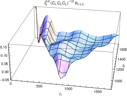
We now numerically compute the bispectrum from recombination and compare it to a local bispectrum [26]. We use WMAP7 parameters: $\Omega_{b}=0.0449$, $\Omega_{c}=0.222$, $h=0.71$, $\tau_{\rm re}=0.088$, $A_{s}=2.43\cdot 10^{-9}$ and $n_{s}=0.963$. Since we want to concentrate on the signal generated at recombination, we do not consider second-order late-time effects such as vector, tensor and RS, that could correlate with the late ISW. As an illustration, in Fig. 4 we plot $b_{l_{1}l_{2}l_{3}}/(C_{l_{1}}C_{l_{2}}C_{l_{3}})^{1/2}$ with $l_{3}=1720$ as a function of $l_{1}$ and $l_{2}$.

To study the observability of the signal, we consider a full-sky cosmic variance limited experiment between $2$ and $l_{\rm max}$, without accounting for lensing. The Fisher matrix between two bispectra $i$ and $j$ is given by [26]

with $\Delta_{l_{1}l_{2}l_{3}}=1,2,6$ for triangles with no, two or three equal sides. We find $F_{\rm rec,rec}=0.225\ (0.504)$, $F_{\rm rec,loc}=0.038\ (0.088)$ and $F_{\rm loc,loc}=0.046\ (0.069)$ for $l_{\rm max}=2000\ (2500)$. The signal-to-noise ratio is given by

most of it is concentrated in the squeezed configuration so that eq. (2) and the local correction (1) capture most of the signal.²² 2 The value of “effective” $f_{\rm NL}$ is given by $(F_{\rm rec,rec}/F_{\rm loc,loc})^{1/2}$. For $l_{\rm min}=100$ we find $f_{\rm NL}^{\rm eff}=-3.82$, which agrees with [13]. However, when $l_{\rm min}=2$ it is smaller, $f_{\rm NL}^{\rm eff}=-2.76$. Indeed, the contamination to a local signal agrees with [19, 20],³³ 3 The local bias computed using eqs. (1) and (2) with $l_{1}\leq 60$ and $10l_{1}\leq l_{2,3}$ is $f_{\rm NL}^{\rm loc}=0.77\ (1.16)$.

and will negligibly contaminate Planck’s searches for local non-Gaussianity.

Discussion: We have presented the most complete calculation of second-order effects at recombination. It confirms that the projection on the local shape from recombination is well described by using the analytic estimate given in [19, 20, 21] and suggests that claims of a large local contamination may be biased by numerical errors. Our calculation did not include lensing and other late-time integrated effects which correlate with the linear ISW effect. Since, for instance, lensing at recombination partially cancels with the rescaling of the coordinates [18, 19], we must include all these effects to correctly estimate the total bias and the observability of the signal. We have shown that CosmoLib$2^{\rm nd}$ is a roboust tool to do this and, more generally, study second-order perturbations in cosmology.

Acknowledgements: We wish to thank F. Bernardeau, P. Creminelli, R. Crittenden, C. Fidler, A. Lewis, G. Pettinari and L. Senatore for useful discussions and suggestions; we are particularly in debt to C. Pitrou for his help and advice on the code CMBquick. ZH is funded by the ANR Chaire d’excellence Junior “CMBsecond”.

References

- [1] http://www.rssd.esa.int/index.php?project=Planck
- [2] D. Hanson, K. M. Smith, A. Challinor, M. Liguori, Phys. Rev. D80, 083004 (2009), arXiv:0905.4732 [astro-ph.CO].
- [3] A. Lewis, A. Challinor and D. Hanson, JCAP 1103, 018 (2011), arXiv:1101.2234 [astro-ph.CO].
- [4] N. Bartolo, S. Matarrese, A. Riotto, JCAP 0606, 024 (2006), astro-ph/0604416. Ibid, JCAP 0701, 019 (2007), astro-ph/0610110. Ibid, astro-ph/0703496.
- [5] C. Pitrou, Class. Quant. Grav. 26, 065006 (2009). arXiv:0809.3036 [gr-qc].
- [6] L. Senatore, S. Tassev, M. Zaldarriaga, JCAP 0908, 031 (2009). arXiv:0812.3652 [astro-ph].
- [7] C. Pitrou, J. -P. Uzan, F. Bernardeau, JCAP 1007, 003 (2010). arXiv:1003.0481 [astro-ph.CO].
- [8] M. Beneke and C. Fidler, Phys. Rev. D 82, 063509 (2010) arXiv:1003.1834 [astro-ph.CO].
- [9] C. Pitrou, www2.iap.fr/users/pitrou/cmbquick.htm
- [10] N. Bartolo, S. Matarrese and A. Riotto, Phys. Rev. Lett. 93, 231301 (2004) arXiv:astro-ph/0407505.
- [11] L. Boubekeur, P. Creminelli, G. D’Amico, J. Norena and F. Vernizzi, JCAP 0908, 029 (2009) arXiv:0906.0980 [astro-ph.CO].
- [12] R. Khatri, B. D. Wandelt, Phys. Rev. D79, 023501 (2009). arXiv:0810.4370 [astro-ph]. Phys. Rev. D81, 103518 (2010). [arXiv:0903.0871 [astro-ph.CO]].
- [13] L. Senatore, S. Tassev, M. Zaldarriaga, JCAP 0909, 038 (2009). arXiv:0812.3658 [astro-ph].
- [14] C. Pitrou, J. -P. Uzan, F. Bernardeau, Phys. Rev. D78, 063526 (2008). arXiv:0807.0341 [astro-ph].
- [15] N. Bartolo, A. Riotto, JCAP 0903, 017 (2009). arXiv:0811.4584 [astro-ph].
- [16] Z. Huang, F. Vernizzi, in preparation.
- [17] Z. Huang, JCAP 1206, 012 (2012) arXiv:1201.5961 [astro-ph.CO].
- [18] P. Creminelli and M. Zaldarriaga, Phys. Rev. D 70, 083532 (2004) arXiv:astro-ph/040542.
- [19] P. Creminelli, C. Pitrou and F. Vernizzi, JCAP 1111, 025 (2011) arXiv:1109.1822 [astro-ph.CO].
- [20] N. Bartolo, S. Matarrese and A. Riotto, JCAP 1202, 017 (2012) arXiv:1109.2043 [astro-ph.CO].
- [21] A. Lewis, JCAP 1206, 023 (2012) arXiv:1204.5018 [astro-ph.CO].
- [22] J. M. Maldacena, JHEP 0305, 013 (2003) arXiv:astro-ph/0210603.
- [23] B. Novosyadlyj, Mon. Not. Roy. Astron. Soc. 370, 1771 (2006) astro-ph/0603674.
- [24] L. Boubekeur, P. Creminelli, J. Norena and F. Vernizzi, JCAP 0808, 028 (2008) arXiv:0806.1016 [astro-ph].
- [25] W. Hu, A. Cooray, Phys. Rev. D63, 023504 (2001). astro-ph/0008001.
- [26] E. Komatsu and D. N. Spergel, Phys. Rev. D 63, 063002 (2001) [astro-ph/0005036].